Inférence bayésienne nonparamétrique pour les densités à support métrique compact et problèmes apparentés

INFÉRENCE BAYÉSIENNE NONPARAMÉTRIQUE POUR LES DENSITÉS À SUPPORT MÉTRIQUE COMPACT ET PROBLÈMES APPARENTÉS

MÉMOIRE PRÉSENTÉ

COMME EXIGENCE PARTIELLE DE LA MAÎTRISE EN MATHÉMATIQUES

PAR.

OLIVIER BINETTE

UNIVERSITÉ DU QUÉBEC À MONTRÉAL Service des bibliothèques

Avertissement

La diffusion de ce mémoire se fait dans le respect des droits de son auteur, qui a signé le formulaire Autorisation de reproduire et de diffuser un travail de recherche de cycles supérieurs (SDU-522 – Rév.10-2015). Cette autorisation stipule que «conformément à l’article 11 du Règlement no 8 des études de cycles supérieurs, [l’auteur] concède à l’Université du Québec à Montréal une licence non exclusive d’utilisation et de publication de la totalité ou d’une partie importante de [son] travail de recherche pour des fins pédagogiques et non commerciales. Plus précisément, [l’auteur] autorise l’Université du Québec à Montréal à reproduire, diffuser, prêter, distribuer ou vendre des copies de [son] travail de recherche à des fins non commerciales sur quelque support que ce soit, y compris l’Internet. Cette licence et cette autorisation n’entraînent pas une renonciation de [la] part [de l’auteur] à [ses] droits moraux ni à [ses] droits de propriété intellectuelle. Sauf entente contraire, [l’auteur] conserve la liberté de diffuser et de commercialiser ou non ce travail dont [il] possède un exemplaire.»

REMERCIEMENTS

Je dédicace ce mémoire à ma famille, à mes amis, mentors et collaborateurs. J'espère que vous saurez--vous-r reconnaitre. __ ~G'est grâce à_votre_soutj_en sé!_ns réserve que j'ai aujourd'hui la liberté d'explorer le riche univers des probabilités et de sés applications à la compréhension de notre monde.

LIST OF TABLES . . . LISTE DES FIGURES RÉSUMÉ ..

ABSTRACT INTRODUCTION

0.1 Subjects of this memoir

0.1.1 Metrics and divergences on probability measures. 0.1.2 Information inequalities ... .

0.1.3 Density estimation using sieve pri6rs 0.1.4 Circular statistics . . .

CHAPTER I

METRICS AND DIVERGENCES 1.1 The total variation distance .

1.2 The Prokhorov metric and weak convergence . 1.3 The Kullback-Leibler divergence . . . .

1.3.1 Exponential convergence of the likelihood ratio 1.4 !-divergences . . . .

1.4.1 Application in importance sampling . . 1.4.2 Application of !-divergences to risk bounds CHAPTER II

REVERSE PINSKER INEQUALITIES 2.1 Abstract ... 2.2 Introduction . 2.3 Main results .. vi Vll viii ix 1 2 2 2 3 8 11 12 13

16

18 20 22 25 31 32 32 33

2.4 Examples . . . . 2.4.1 Relative entropy (Kullback-Leibler divergence) . 2.4.2 Hellinger divergence of order a

2.4.3 Rényi's divergence 35 35 36 36 2.5 Proofs . . . 37 CHAPTER III

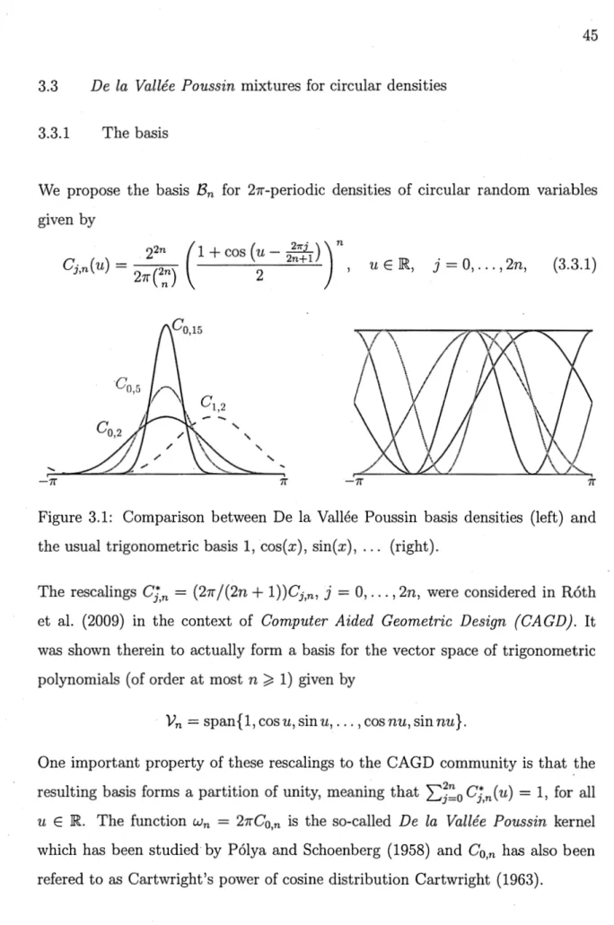
BAYESIAN NONPARAMETRICS FOR DIRECTIONAL STATISTICS . 41 3.1 Abstract . . . 42 3.2 Introduction . . . 42 3.3 De la Vallée Poussin mixtures for circular densities

3.3.1 The basis ... . 3.3.2 The circular density model . 3.4 Prior specification ... .

3.4.1 Circular density prior . 3.4.2 Strong posterior consistency

3.4.3 Relationship with Dirichlet Process Mixtures . 3.4.4 Adaptative convergence rates

3.5 Comparison of density estimates . . . 3.5.1 Nonnegative trigonometric sums. 3.5.2 Methods . 3.5.3 Results . 3.5.4 Implementation summary 3.6 Discussion . 3. 7 Appendix A 3.7.1 Proof of Theorem 3.4.3 . 3.8 Appendix B . . . . 3.8.1 Proof of Theorem 3.4.4 . 45 45 47 52 52 54 55 57

60

60

61 62 67

68

69

69

73 73

3.9 Appendix C . . . . 3.9.1 Auxiliary results

76 76

Table Page · 1.1 Common !-divergence definitions and related fonctions. . . 21

Figure Page 3.1 Comparison between De la Vallée Poussin basis densities (left) and

the usual trigonometric basis 1, cos(x), sin(x), ... (right). . . 45 3.2 The Skewed von Mises family of densities (left panel) and the

w-family of densities (right panel). . . 63 3.3 Mean Kullback-Leibler losses for the Skewed von Mises family { v0 }

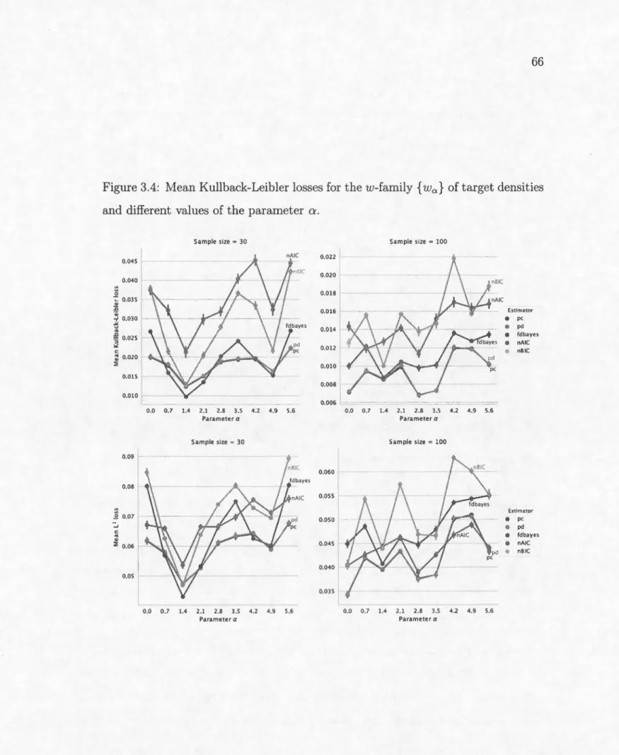
of target densities and different values of the parameter a. . . . . 65 3.4 Mean Kullback-Leibler losses for the w-family { w0 } of target

den-sities and different values of the parameter a. . . 66 3.5 Examples of density estimates for different tàrgets and sample sizes. 67

Le thème principal de ce mémoire est l'estimation de densités définies sur des es-paces métriques compacts en utilisant des méthodes bayésiennes nonparamétriques (Binette and Guillotte, 2018). Le cas où l'espace métrique est le cercle, d'intérêt en statistique circulaire et directionnelle, est développé avec une attention par-ticulière. Nous proposons dans ce contexte une base de densités de probabilités des polynômes trigonométriques possédant des propriétés de préservation de la forme analogues aux densités polynomiales de Bernstein. Une étude de simula-tion montre que des estimateurs bayésiens nonparamétriques développés à l'aide de cette base peuvent offrir des gains par rapport à des méthodes comparables précédemment suggérées dans la littérature.

D'un point de vue théorique, nous étudions les propriétés de concentration, pour la distance de Hellinger, des distributions a posteriori issues de modèles engendrés par des opérateurs d'approximation linéaires positifs de rang fini. Ce type de modèles généralise les polynômes aléatoires de Bernstein à l'utilisation d'autres types de bases de densités de probabilités définies sur des espaces métriques com-pacts arbitraires. Ceux-ci se prêtent particulièrement bien à l'estimation sous con-traintes de formes et les calculs a posteriori peuvent généralement être effectués à l'aide du Slice Sampler de Kalli et al. (2011). Nous obtenons la convergence de la distribution a posteriori sous des conditions de régularité particulièrement faibles ne nécessitant pas d'hypothèses de continuité. Des vitesses de convergences adap-tatives sont de plus obtenues en termes de la croissance du rang des opérateurs et de leurs propriétés d'approximation.

Ces contributions sont liées à quelques bases mathématiques présentées dans le premier chapitre. Nous y introduisons différentes fonctions connues de divergences sur des ensembles de mesures de probabilités ainsi que leur relation au rapport de vraisemblance. De nouvelles inégalités de type Pinsker inverse, permettant d'obtenir des bornes optimales sur les /-divergences en termes de la variation totale et des extremums du rapport de vraisemblance (Binette, 2019), sont dérivées dans le Chapitre 2.

This work is concerned with density estimation on compact metric spaces using sieve priors (Binette and Guillotte, 2018). Particular attention is given to the case where the metric space is the circle as the problem is relevant to circular and di-rectional statistics. In this context, we suggest a density basis of the trigonometric polynomials that is analogous, beca:use of its interpretability and shape-preserving properties, to the Bernstein polynomial densities. A simulation study shows that the use of Bayes estimators constructed using this basis may provide gains over comparable circular density estimators previously suggested in the literature. From a theoretical point of view, we study the convergence of posterior distribu-tion, in the Hellinger sense, for models that arise as the images of positive linear approximation operators with finite ranks. These models generalize random Bern-stein polynomials to the use of other density bases defined on arbitrary compact metric spaces. They are particularly well suited to shape constrained density es-timation and posterior simulation may be carried out using the Slice Sampler of Kalli et al. (2011). Strong posterior consistency is obtained under notably weak regularity assumptions and adaptative convergence rates are expressed in terms of the growth of th~ operator ranks and of their approximation properties. Sorne mathematical background is introduced in the first chapter. We introduce different known divergence fonctions over sets of probability measures as well as their relationship to the likelihood ratio. New reverse Pinsker inequalities, providing optimal upper bounds on !-divergences in terms of the total variation and likelihood ratio extremums (Binette, 2019), are derived in Chapter 2.

Suppose that some unknown mechanism iteratively generates data points X1 , X2 , X3 , and so on. Our goal is to use finitely many of those observations, say (Xi)i=I,

to infer characteristics of the mechanism that may be of interest.

The way in which the points Xi are generated can be arbitrarily complex and may stochastically depend on external factors. The starting point of any meaningful statistical analysis would therefore be an assessment of the dependencies involved. In the simplest case, which still abstractly encompasses a number of more general situations, we model the points Xi as random variables that are independent and identically distributed following some unknown probability distribution P0 •

Our

epistemic uncertainty about what may be P0 is quantified through what is

called a prior probability distribution II over the set of all reasonable possibilities for what Po may be. Given a set A of probability distributions, the prior prob-ability II(A) of A specifies what we consider as the probprob-ability that "Po E A"

before any observation of the Xi has been made.

Once we have observed the data points (Xi)i=I' we may adjust our prior quantifi-cation of uncertainty about Po through probabilistic conditioning, thus obtaining what is called the posterior distribution A.-+ II (A 1 (Xi)f=_1).

This process of first quantifying uncertainty over an unknown state of the world through a prior probability measure and then making adjustments using the

cal-culus of probabilities in light of new observations is called Bayesian inference. 0.1 Subjects of this memoir

0.1.1 Metrics and divergences on probability measures

Our first chapter introduces some mathematical ideas relevant to the theoretical developments of the following chapters. We discuss different metrics and topolo-gies on the space

M

of all pro babili ty measures on the space M on w hich the variables Xi take values, as this is related to the definition of prior distributions on

M

and to the study of properties of the posterior distributions.

0.1.2 Information inequalities

In chapter· 2, we derive new best-possible inequalities allowing us to upper bound !-divergences in terms of the total variation distance and of likelihood ratio ex-tremums. This work can be inscribed in the field of Information Inequalities: this is about relating together different distributional characteristics of the log likelihood ratio.

The motivation cornes from Bayes' Theorem, which states that, in dominated models, the posterior distribution II(· 1 (Xï)f=_1), for independent observations Xi

with density fo, may be written as

TI(A 1 (X;)f~1) ex

i

ü

fa~~:)

TI(df). (0.1.1)

The two elements involved in the right-hand sicle of this formula are the prior distribution II and the likelihood ratio

f / f

O• The logarithm of this likelihood ratio is commonly referred to as the "information" fonction L(x)

=

log

Jo~~)

and we are interested in its distribution for x a random variable with density fo. The study of the behaviour of posterior distributions is therefore typically based on

properties of Il, on characteristics of the distrib11:tion of the information

i(x)

over the range

f

E lF and on the .resulting geometry on lF. Characteristics of l include

the total variation between fo and f, their Renyi divergence and their Kullback-Leibler divergence. Each may be expressed as an expected convex transform of exp l(x); they are what are called f-divergences.

Information inequalities relate together different characteristics of l as well as the

resulting geometries on lF. They are quite fondamental to the study of posterior distributions. One such inequality, of which we make repeated uses in Chapter 3, is

j

fo log ; ( sup ; )

j

If - fol.

This is an instance of a reverse Pinsker inequality: it upper bounds an f-divergence in terms of the total variation distance and the extremums of the likelihood ratio. While the above is immediate and already quite useful, it can be significantly improved. In Chapter 2, it is shown that any f-divergence D</J, here characterized by a convex fonction cjJ :

[O,

oo)

-+ 1î with

c/J(l)

=

0

and

D~(Jo, J)

=

lE [ (/)

(fa~~))],

x

~

fo, we have

sup D</J(Jo, f)

=

8 (

c/J(m)

+

cjJ(M) )

(!0,f)EA(m,M,8) 1 - m M - 1

when considering the class A(m, M, 8) of pairs Uo, f) satisfying inf f / fo

=

m,

sup f / fo

=

M and

J

If - fol

=

28. This idea is developed in Binette (2019) as a response to suboptimal particular cases that appeared in the information inequalities literature.

0.1.3 Density estimation using sieve priors

Chapter 3 considers in some generality the case where the variables Xi take val-ues in a compact metric space (M, d). For instance, the variables Xi may be

observations of angles distributed on the sphere or of directions distributed on a sphere.

We exploit sequences Tn : L1 _{(M) L}1 _{(M), n E N, of positive linear opera tors} with finite ranks mapping IF to IF in order to obtain the decomposition

IF=

LJ

Tn(IF),

nEN

where the overline denotes L1 _{closure in IF. Given prior distributions Iln on the} submodels Tn(IF) and a distribution p on N, we thus obtain a prior Il on IF through

Il=

L

p(n)Iln. (0.1.2)

nEN

This is an instance of a sieve prior or mixture prior and a number of particular cases have appeared previously in the literature. Let me showcase a few examples · and explain how some of our general results of Chapter 3 can easily be used to obtain asymptotic properties of the posterior distribution in terms of simple properties of the opera tors Tn.

Random Bernstein polynomials.

With M

=

[O, 1], take Tn the Bernstein-Kantorovich operator defined as

~1*

Tnf: x 1-t (n

+

1) L...J i f(u) dupi,n(x),

i=O n+l

where Pi,n(x)

=

(7)xi(l - xt-i is the ith Bernstein polynomial of degree n. It follows that

Tn(IF)

=

{(n+

1) tCj,nPj,n: Cj,n;;?, 0, Lcj,n

=

1}

i=O J

is the set of fini te mixture of Bernstein polynomial densities of degree n. With Iln a Dirichlet distribution on the coefficients ( Cj,n) with parameters for instance Œj,n

=

case of the random Bernstein polynomials of Petrone (1999). Theorem 3.4.3 entail · strong posterior consistency at all bounded densities provided also that

p(

n)

>

0 for every n E N. Theorem 3.4.4, together with the well-known fact that IITnf

-f

11₀₀

=

0 (w1(n-1!2)) where WJ is the modulus of continuity of

J,

yields the

posterior contraction rate én

=

(n/ log(n))-.B/(2.B+2) whenever log p(n) ::=::: -nlogn

and the data generating density

f

O satisfies the the Holder continuity condition w₁₀(8) C8.B for soine C

>

0 and (3

>

O. The strong posterior consistency result refines Theorem 2 of Petrone and Wasserman (2002) by removing continuity assumptions on fo while the posterior convergence rate we obtain is the same, up to log factors, as that obtained in Kruijer and van der Vaart (2008). However, the generality of our approach makes it readily applicable in other contexts as well.

Random histograms on metric spaces. Let M be an arbitrary compact

metric space and let {Rj,n}J:;;,₀ be a measurable partition of M of diameter less than n-1 _{with d~ E N elements. We assume that maxi µ(Rj,n)-}1

=

_{O(dn) and}

that dn is an increasing integer sequence satisfying dn ::=::: nd for some d

>

O. Define

dn

r

Tnf: X

HE

}r,

f(u)duµ(Rj,n)-1]Rj,n(x) j=O Rj,n so that Tn(JF)

=

{t

Cj,n µ(Rj,n)-1llR;,n : Cj,n

0,

E

Cj,n

=

1}

J=O J

and IITnf -

Jlloo

=

O(w1(n-1 )) _{for any continuous}

J.

_{With Iln a Dirichlet}

distri-bution on the coefficients ( Cj,n) with parameters Œj,n

=

1/

dn and p a distribution

on N satisfying log

p(

n) ::=::: -dn log( dn), we obtain from Theorems 3.4.3 and 3.4.4

strong posterior consistency at any bounded density and the posterior conver-gence rate ên

=

(n/ log(n))-.B/(2.B+d) provided that fo satisfies a Holder continuity condition with exponent (3

>

O.

and piecewise constant fonctions can be replaced by many other types of basis fonctions: splines with fixed knots, Gaussian kernels at predetermined locations, etc. The properties of resulting posterior distributions are then studied through the associated sequence of positive linear operators.

By the Riesz representation Theorem (Rudin, 1987), any positive linear operator and such that Tn ( 1)

=

1 takes the form

Tnf: x H 1E [f (Yn(x))] (0.1.3)

for some families {Yn ( x) : x E

M}

of random variables. In the examples considered above, it is an easy exercise to explicita definition of Yn(x). The expression (0.1.3) is especially useful when required to obtain the approximation rate of Tn- Indeed, suppose that the modulus of continuity of

f

satisfies WJ(n8) nwJ(8) for any n E N and 8

>

O. This is the case, for instance, when M is a smooth compact

submanifold of Euclidean space together with its geodesic distance. Then for any sequence 8n 0 we have that

IITnf -

flloo

WJ(8n) {2

+

8;;1 suplE _xEMI [d(Yn(x), x)]d(Yn(x),x)~on]} WJ(8n) sup {2

+

8;;2 sup lE [d(Yn(x), x)2]}.

xEM xEMI

We may show that supxEMI 8;1_{IE[d(Yn(x), x)] is uniformly bounded in n, which}

therefore entails that

IITnf -

flloo

=

O(w1(8n)).

The square of the distance fonction is easier to deal with in some cases, such as when d(x, y)

=

lx -

YI

on [O, 1]. In this case, if supxEMI IE[d(Yn(x), x)2] a~ for some sequence of "variances" a~ E IR, then by letting 8n

=

a;

1 _{we obtain that}

This relates the uniform contraction rate of the variables Yn ( x) around x to the approximation rate of Tn.

Interpretability and shape constrained estimation. It is notoriously

difli-cult to elicit priors on infinite dimensional spaces. The use of a sieve priors such as (0.1.2) reduces the problem to that of eliciting a prior on the finite dimensional subsets Tn(lF), which always admit a representation of the form

Tn

(JF)

= {

t

Cj,n <Pi,n}

J=Ü

for some basis densities c/Jj,n and coefficients Cj,n, and a prior p on the parameter

n. This parameter n may be thought as representing the complexity of the sieve through its dimension dn. The asymptotic theory of Chapter 3 suggests taking p(n) ::::::::: -dn log(dn) or p(n) ::::::::: -dn, and also provides some guidance for the choice of the prior on Tn(lF). The Bayes estimator resulting from (0.1.2) is simply the mixture of the Bayes estimator obtained from the priors IIn on Tn(lF), weighted by the posterior probabilities of each model.

In some cases, the operators Tn may be extended to act upon probability mea-sures; see again Chapter 3 for more details. If V is a Dirichlet Process, then the

prior induced by the random density TN(V) where N rv pis independent of Vis

bath a Dirichlet Process Mixture and a sieve prior as in (0.1.2). The interpretation as a Dirichlet Process Mixture is especially useful in view of the computational methods developed in Kalli et al. (2011). The sieve prior representation is oth-erwise typically more suited to reversible jump MCMC algorithms for posterior simulation.

We may also want to incorporate very precise types of prior information into the model. For instance, if fo is defined on

M

=

[0,

1

]2,

we may know a priori its marginal distributions. Or we may know that fo defined on

[O,

1] is monotonous.

The sieve prior (0.1.2) is particularly well suited to the incorporation of such shape constraints.

Indeed, it suffices restrict IF to be the set of all bounded densities satisfying the required shape constraint, and tolet Tn be such that Tn(IF) C IF. This is possible in mentioned particular cases, e.g. for copula density estimation and monotone density estimation. The theory continues to apply in this context with still the same interpretability and with rates of convergences depending on the dimensions of Tn(IF).

0.1.4 Circular statistics

The above theory has been developed concurrently to the study of a circular ana-logue to the Bernstein polynomial densities which we use in Chapter 3 to" construct sieve priors on circular density spaces. The density basis of the trigonometric polynomials that we consider is given by

cj,n(u)

ex

(1

+

cos

(u -

2!711)

r

with a known normalizing constant and j E {0, 1, 2, ... , 2n }. The central element Co,n is, up to a multiplicative constant, the De la Vallée Poussin kernel studied in Polya and Schoenberg (1958). The consideration of this set of translates was proposed in Roth et al. (2009) in the context of Computer Aided Geometric De-sign. Here we have studied properties of Cj,n which are particularly relevant to mixture modelling.

As such, we provide the Fourier coefficients of Cj,n which are also referred to in the directional statistics literature as the trigonometric moment~. These provide • the change of basis formula between the Ci,n and the usual trigonometric basis {1,

cos(u),

sin(u), ... ,

cos(nu),

sin(nu)}. Together with the method for the effi-cient simulation of the

Cj,n

provided in Chapter 3 and the characterization of

positive trigonometric densities

as

mixtures of the Cj,n, this shows how any

posi-tive trigonometric density can be directly simulated as a mixture and provides an algorithm to do so.

Sorne properties of a mixture density

f

= ~;:

0 Cj,nCj,n, where Cj,n 0, ~i Cj,n

=

1, can also be easily related to properties of the vector of coefficients (

Cj,n)J~o-Those can be neatly stated in terms of properties of the operator 2n

Tnf

=

L

1

f(u)duCj,n

j=O Rj,n

(0.1.4) with Rj,n

= [

rr~;_;

₁1),

rr~;:

₁1)). Using variation diminishing properties of the De la Vallée Poussin kernel studied in Polya and Schoenberg (1958), it is shown in Chapter 3 that

Tn

reproduces constants, that it preserves periodic unimodality and diminishes total variation. Furthermore,

IITnf -

!11

00 0 as

n

oo for

every conti11:uous

f.

The same kind of properties hold for the De la Vallée Poussin means

Vnf(x)

= ["

f(x - u)Co,n(u)du

for which it is also known that

IIVnf -

Jlloo

=

O(w1(n-1_{!2 )) (Lorentz, 1986).}

Approximation rates can be obtained for

Tn

defined in (0.1.4) using the technique described in Section 3.4.4.

In order to showcase the practical usefulness of these densities and of the frame-work which we used to construct sieve priors, we have compared the finite sample performance of our Bayes estimators to other circular density estimators based on trigonometric polynomial densities. Notably, Fernandez-Duran (2004) used a surjective parameterization of the space of all trigonometric densities through a complex hypersphere in order to compute maximum likelihood estimators. Model dimensions are chosen using the AIC or BIC criteria. In Fernandez-Duran and Gregorio-Dominguez (2016a), posterior means are also considered. The density

estimators based on our models provide the best performance in a variety of sce-narios. These results are not meant to show that our estimators are best-possible, but simply that the De la Vallée Poussin basis should be considered for circular density modelling, especially when there is an availability of prior information to support informed Bayesian estimation.

Let (M, d) be a complete and separable metric space together with its Borel

Œ-algebra œM and let

M

be the space of all probability measures on (M, œM). This section presents elementary facts about

M

and its common metrics and topologies, some of which may be found in Aliprantis and Border (2006); Ghosh and Ramamoorthi (2003a); Gibbs and Su (2002); Billingsley (2013).

1.1 The total variation distance

The space

M

embeds in the ( complete) normed linear space of measures µ with finite total variation

llµIITv

=

sup AE'BM

lµ(A)

1 and inherits the total variation

distance dTv(µ, v)

=

Ilµ - vllTv· While this metric is- easily interpretable as mea-. suring worst case difference in mass allocation, it is so at the loss of tractability of the resulting metric space:

M,

with the total variation distance, is not separable unless M is countable. 1

However, the problem disappears when considering dominated subsets of

M

as such sets identify with part of a suitable L1 _space.

Lemma 1.1.1. A subset F

CM

is dominated by a Œ-finite measure if and only if

(F,

drv) is separable.

Proof. First suppose Fis dominated by a Œ-finite measure À. Take µ, v E F and consider the densities (i.e. Radon-Lebesgue-Nikodym derivatives)

f

=

dµ/ dÀ,

1_{To see this non-separability, suppose M is uricountable and consider the subset { ôx} xEM} of point mass measures. Let also E C M be such that for every x E M, there exists Vx E E

with llôx - vxllTv < 1/2. It follows that Vx must contain a point mass at x. Since Vx is finite, it

contains only a countable number of such point masses. Any countable number of such measures can only approximate in this way a countable subset of {ôx}xEM· This shows E is uncountable and hence M is not separable.

g

=

dv/dÀ in L

1

(À). The set A

=

{x E M

I

f(x) g(x)} E

œM

is such that

Ilµ - vllTv

=

(µ -

v)(A)

=

(v - µ)(M\A) and it follows that

Ilµ - vllTV

=

j

If - 91

d>..

(1.1.1) Hence dTv is equivalent to the L1 _{distance on the identification of F with its} densities {dµ/dÀ 1 µ E F} C L1(À). Since À is a-finite and

œM

countably

generated, L1_{(À) is separable and so must be (F, dTv ).}

Conversely, if (F, dTv) is separable, let E

=

{µn

I

n E N} be a countable dense

subset of

F.

We show that À= LnEN µn2-n dominates

F.

Let A E

œM

be such that À(A)

=

0, fix µ E F and ê

>

O. Then µn(A)

=

0 for every n and by density

of E there exists a n E N such that µ(A)

=

lµ(A) - µn(A) 1

<

ê. Since ê

>

0 was

arbitrary, µ(A)

=

O. This shows µ

«

À for every µ E

F.

1.2 The Prokhorov metric and weak convergence

Asto obtain a complete separable metric structure on

M

we may relax the total variation distance the Prokhorov metric d p. l t is deffned as

dp(µ, v)

=

inf{ ê

>

0

l

'v A E

œM,

µ(A) v(Aé)

+

ê} (1.2.1) where At:

=

{x E M

I

d(x, A)

<

ê} is the ê-neighborhood of A and d(x, A)

=

inf{d(x, y) 1 y E A} (Strassen, 1965; Prokhorov, 1956). This provides a

metriza-tion of the topology of weak convergence of probability measures (see for isntance Hu ber ( 2011)), also known as the weak-* topology of the continuo us dual of Cb (M), which is further described by the Portmanteau theorem (see Billingsley (2013)). It follows from (1.2.1) that dp dTv• Hence total variation convergence implies weak convergence. The converse obviously does not hold, as can be seen by considering the sequence of measures µn

= ¾

I:~=l

Ôi/n defined on [O, 1] C R

While

{µn}

does not converge in

(M,

dTv ), it converges to the Lebesgue measure in (M, dp ). The approximation properties of measures with finite support are further discussed in the proof of the following lemma.

Lemma 1.2.1. The space

(M,

dp) is separable if and only if (M, d) is separable. Proof. Suppose

(M,

dp) is separable and consider the map cp: MI-+

M :

x r-+

ôx.

Fix x,y E M and let

ê

=

min{d(x,y),l}. The fact that c5x({x})

c5y({AY) +ê

shows dp(cp(x), cp(y)) ;?; ê and obviously

ôx(A) c5y(A

8)

+

c5 for every c5

>

ê and A E ~M- Hence dp(<p(x),cp(y))

=

min{d(x,y), 1} and <p establishes an isometry between (M,

J).

and

(M,

dp) when

d

=

min{ d, 1 }. Thus (MI,

d)

is separable and so is the homeomorphic (MI, d).

Now suppose (M, d) is separable and let E be a countable dense subset. We show that

{L7=

1

aiôxi

I

n E N, ai E (Q, Xi E E} is dense in

(M,

dp). To this end, fix ê

>

0 and let µ E

M.

Let n E N and

{xi}i=l

C E be such that

µ (MI\

u~=l

B(xi,

ê)) <

ê/2 and consider V

=

I:7=1 Ü'.iÔxi

where Ü'.i E <Q is such that

lai -

µ(B(xi, ê))I

<

ê/(2n). Then for any A E ~M,

n

µ(A)~

i

+

Lµ(B(xi,ê/2)

n

A)~

ê +

L ai= v(Ae)

+ ê

i=l XiEAe

which shows dp(JL, v) ê.

The following theorem provides coupling characterizations of the two metrics seen thus far and highlights how exactly d p weakens dTv by taking into account the metric structure of MI. A proof can be found in Dudley ( 2002) and here we denote A8_l

=

_{{x E}

MI

_{d(x,A) c5}.}

Theorem 1.2.2 (Strassen (1965) ). Letµ, v E

M

and let

C

be the set of all pairs

space of probability measure If!>) with marginal distributions µ an~ v, respectively. Then for every ë, 8 0 following two statements are equivalent:

(i) for every A E ŒM, µ(A)

v(A

6

l)

+

ë;

(ii) there exists

(X,

Y) E C such that If!>

(d(X,

Y)

>

8)

ë.

Considering the cases 8

=

0 and 8

=

ë yields explicit descriptions of dTv and dp.

Corollary 1.2.3. Letµ, v and C be as in Theorem 1.2.2. Then

and

drv(µ, v)

=

inf

{ë >

0 1 If!>

(d(X,

Y)> 0)

ë}

(X,Y)EC

dp(µ,v)= inf

{ë>OIIP(d(X,Y)>ë)~ë}.

(X,Y)EC ·

We conclude the presentation of (M, dp) with a simple measurability result rele-vant to the definition of random probability measures.

Lemma 1.2.4. The evaluation maps M 3 µ H µ(A), where A E ŒM, are Borel measurable.

Proof. The definition of dp entails the map f

(µ)

=

µ(A) is upper semi-continuous whenever A is a closed set. Indeed, fix µ0 E M, ë

>

0 and let 8

>

0 be such that

8

<

ë/2 and µ0(A6\A)

<

ë/2. Then by definition dp(µ, µ0 )

<

8 implies µ(A)

-µ0(A) µ0(A6\A)

+

8

<

ë. Since semi_;continuous functions are measurable, this shows the family

A

of sets A E ŒM such that µ H µ(A) is measurable contains

the 1r-system of closed sets of M. It is immediate to verify

A

is also a À-system. From-Dynkin's theorem, we obtain that

A:)

ŒM.

1.3 The Kullback-Leibler divergence

We now turn to another measure of discrepancy between probability measures, introduced by Kullback and Leibler (1951).

To motivate its definition, let À,µ, v E

M

and consider the problem of testing

H1 : À

=

µ versus H2 : À

=

v given an i.i.d. sample {

Xi}i=I

of size n E N with common distribution À. We write X

=

(X_{1 , ... ,} Xn) rv À(n). Assuming µ, v and À are mutually absolutely continuous2 , we can define their likelihood ratio as

n d

dµ

(X)

:=

IJ

_!!:_(Xi)

E

[O,

oo].

dv _i=l . dv (1.3.1)

The weight of evidence brought by the sample X in favor of H1 versus H2 is defined as W(X)

=

log ~(X) (Good, 1985). This is also known as the relative information of X according to (µ, v) (Sason and Verdu, 2016), and is the usual statistic of the likelihood ratio test.

The Kullback-Leibler divergence D(µllv) between µ and vis the expected weight of evidence brought by a single observation taken under the hypothesis H1 (taking the expectation under H2 simply reverses the sign). In the words of Kullback and

Leibler, it is the "mean information for discrimination between H1 and H2 per observation". Hence formally

D(µllv)

=

L

log ( dµ. (1.3.2)

When µ, v are not absolutely continuo us with respect to one another, we define

D(µllv)

=

oo. This case does not always require particular care as we may introduce

ç

= µ

+

v and write D(µllv) = Jf>O

f

log(! /g)dç with

f

= dµ/dç and

2_{This assumption is not completely necessary, but it is enforced here as to simplify the}

g

=

dv / dç. Equation (1.3.2) is well defined as the integral of the negative part of the integrand is bounded:

1 (

dµ)

1

(dv )

- log - dJJ, - - l dJJ,

{dµ/dv<l} dv {dµ/dv<l} dµ

=

v( {~µ/dv

<

1}) - µ( {dµ/dv

<

1})

<

1.

The following theorem shows that the magnitude of D is a statistically meaningful quantity. Here we let Y be some measurable space and T : M M a measurable transform. We denote by µT-1 _{the pushforward measure defined by µT-}1_(A)

=

µ(T-1_{(A)) for Ac Y measurable.}

Theorem 1.3.1 (Kullback and Leibler). Ifµ, v E M are absolutely continuous with respect to one another and if T : M Y is a measurable transform of M, then D(µT-1_{llvT-1) D(µllv) with equality if and only if T is a sufficient}

statistic for {µ, v}.

Proof. To ease notation, write

µ

= µT-1 ,

v

= vT-1 and let h

=

Î/(f/;

o T).

Remark that by change of variable

D(µllv) - D(,üllii)

=

L

(log

(t) -

log(~ o T)) dµ

=

L

log(h) dµ. Since

JM

l/h dµ

=

l, Jensen's inequality together with the convexity of the func-tion ef>(t)

=

t

log(t) yields D(µllv)-D(P,llv) ef>(l)

=

0 with equality if and only if

h = l µ-almost surely. Hence equality happens if and only if

Î

=

fi;

o T µ-almost

everywhere which, since µ

«

v and v

«

µ, amounts to saying T is sufficient for·

{µ,

v} (Halmos and Savage, 1949, Theorem 1).

Considering the case where T is constant yields an equally important result.

Corollary 1.3.2. Ifµ, v E

M,

then D(µllv) 0 with equality if and only if

1.3.1 Exponential convergence of the likelihood ratio

The importance of the Kullback-Leibler divergence in Bayesian nonparametrics and asymptotic statistics stems from its characterization of the likelihood ratio's exponential convergence.

Proposition 1.3.3. Suppose µ, v E M are absolutely continuous with respect to one another and let { Xi

I

i E

N}

contain independent random variables with distribution µ. The f ollowing two statements are equivalent.

(i) D(µllv)

<

oo.

(ii) There exists an RE (0, oo) such that

f1~

₁

~(Xi)=

exp {nR

+

o(n)} almost surely.

Also, when the statements hold, we have R

=

D(p,llv) in (ii).

Proof. Note that (ii) is equivalent to

¼

I:~=

1 log

~(Xi)

=

R

+

o(l)

almost surely for some R E

[O,

oo). By the Strong law of large numbers, this happens if and only if R

=

1E [log

~(Xi)]

=

D(µllv).

Given a bound on the second moment of dµ/dv also provides a stochastic control on the fluctuations of the likelihood ratio. Here we state a result of this kind which is particularly helpful to the study of posterior distribution.

Lemma 1.3.4 (Lemma 8.1 of Ghosal et al. (2000)). Let Il be a prior on a subset IF of

(M,

drv) with respect to its Borel Œ-algebra. Fix E

>

0, 81

>

0, 82

>

0 and · let W

=

{µ

E lF

I

J

log ~;dv :(

ch,

J

(log

;;;:)2

dv :( c52}. If

(X;)f=1

is a sequence

of independent random variables U?ith distribution v, then

1

IT

(X;)II(dµ) ;;:, e~n(.i'.+e)rr(W)

W i=l

holds with probability at least l -. né

<5\ .

Remark 1.3.l. The Lemma shows how the Kullback-Leibler divergence, here con-trolled through the constant 81, provides a probable exponential bound on the convergence of (an average) of the likelihood ratio. The second moment bound 82 of the log likelihood ratio acts linearly on the probability of the lower bound. Proof ofLemma 1.3.4. Assume, without loss of generality, that

II(W)

>

0 and let

fi

=

II/II(W)

be the renormalization of II over

W.

By Jensen's inequality,

{ n d n { d

log

J~

IT

d~ (Xi)ÏI(dµ) ;:;,

L

J~

log

d~ (Xi)ÏI(dµ)

W i=l i=l W

and hence the complementary probability of (1.3.3) is

1P'

(L

Il~~

(X;)Ïl(dµ)

e-n{J,+e)) 1P'

(t

L

log~~

(Xi)ÏI(dµ) -n(8

1

+

e:)) .

~ubtracting the average E

=

-n

fw

D(vllµ)IT(dµ) of

I:~=1

fw

rr~=l

~(Xi)II(dµ)

and using the fact that E -n<51 , this is upper bounded by

1P'

(t

L

log

!~(X;)ÏI(dµ)- E ~.

-ne:)

1P' (

(t

fw

log

dv(xi)ÏI(dµ)-

E)

2

(ne:)2)

n~2

E [

(Llog

!~

(Xi)fi(dµ))

2 ]

where the last inequality follows by Chebychev's inequality. By Jensen's

inequal-( d ~ )

2 _{d 2 ~}

ity,

fw

log

J,;(Xi)II(dµ)

fw

(log

J,;(Xi)) II(dµ)

and by Fubini's theorem and the definition of W we obtain that the expectation of

fw

(log

~(Xi))

2

II(dµ)

1.4 !-divergences

A large and very useful family of measures of discrepancy between probability measures is obtained by considering expected transforms of the likelihood ratio. The basic idea is that, for the purposes of likelihood based inference, any mean-ingful measure of distance or discrepancy between probability measures should be fun:ction of their likelihood ratio. In particular, expected convex transforms of the likelihood ratio encompass a number of useful particular cases and share useful properties.

Definition 1.4.1. Let

f :

[O,

oo)

--+

(-oo, oo)

be a convex function which is strictly convex at 1 and such that

f

(1)

=

O. Given two probability measures

µ, v E M such that µ

«

v, the !-divergence between µ and v is defined as

D1(µ1iv)=IEvH:~)]

=

J

i(dv)dv.

(1.4.1)

Remark 1.4.1. Part (i) of Proposition 1.4.2 shows that D_I is well-defined: while it may be infinite, the integral of the negative part of f(dµ/dv) with respect to v is always finite.

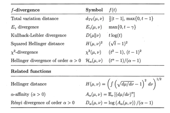
Table 1.1 summarizes a few of the most common !-divergences.

Remark 1.4.2 (Hilbert interpretation). Let IF be a separable subset of (M, dTv)

and let À be a dominating o--finite measure. While IF is naturally identifiable with part of L1

_(À)

_{(see the proof of Lemma 1.1.1), the identificationµ M E}

L2_{(À) with part of the unit sphere of the Hilbert space L}2_{(À) provides additional}

tools. The resulting inner product of L2 _{is referred to as the (1/2)-affinity defined}

by

A1;2(µ, v)

= /

_\ Jdv/dÀ) _L2(>.) .

and the L2 ( À )-distance for root densities is referred to as the Hellinger distance H(µ,v)

=

Table 1.1: Common /-divergence definitions and related functions.

/-divergence

Total variation distance E'Y divergence

Kullback-Leibler divergence Squared Hellinger distance

x

2

-divergence

Hellinger divergence of order a

>

0

Related functions

Hellinger distance a-affinity ( a

> 0)

Rényi divergence of order a

>

0

Symbol f(t) dTv(µ, v) ½lt -

lj,

max{O, t -

1}

E-y(µ, v) max{O, t - ,} D(µllv) tlog(t) H(µ, v)2

( Jt-1)2

x2(µ, v) ( t2 - 1), ( t - 1) 2 1-la(µ, v) ( t0 -

1) / (

a -

1)

( ....--- 2 ) 1/2 H(µ,v)

=

f (

Jdµ/dv-1) dv Aa(µ, v)

=

IEv [(dµ/dv)°]

Da(µ, v)

=

log (A0 (µ, v))

/(a -

1)

These quantities are monotonous transforms of the Hellinger divergence, of the Rényi divergence and of a-affinity.

Proposition 1.4.2. Let D f be any /-divergence, as in Defiriition 1.4.1. (i) IEv [max{O, - f (dµ/dv)}]

<

oo

(ii) We have D1(µllv) 0 with D1(µllv)

=

0 if and only ifµ= v.

(iii) If T is any measurable transform of M, then D1(µllv) D1(µT-1, vT-1)

with equality if and only if T is a sufficient statistic for {µ, v}.

f (

t)

0 for every 0

t

1. In the first case,

lEv [max{0,

-f

(dµ/dv)}] lEv [-

f

(max{dµ/dv, 1} )]

-f

(IEv [max{dµ/dv, 1}])

<

oo. by Jensen's inequality. The second case follows similarily.

Taking T any constant fonction, {ii) is seen to be a particular case of {iii). In order to prove {iii), let

µ

=

µT-1 , f;

=

vr-

1 and note that

[dµ ]

dv (y)

=

lEx~v dv (X) 1 T(X)

=

y .

Hence using Jensen's inequality and with X '"'"' v we find

D1(µllv)

=

JE

H

!~(X))]

=

JE [JE

[1

(dv(x))

1

T(X)]]

JE

[1 (

JE

[!~(X)

1

T(X)])]

=

JE

[1 (:

(T(X)))]

=

D1(J:illîi).

Since

f

is strictly convex at 1, equality holds if and only if

=

1/g

o T v-almost everywhere. Because µ

«

v, this is the same as saying that T is a suffi.dent

statistic for

{µ,

v} (Halmos and Savage, 1949, Theorem 1). 1.4.1 Application in importance sampling

One particularly accessible and useful subject in which !-divergences appear is in error quantification for importance sampling. Without delving very deep in the theory (see Chatterjee and Diaconis (2018); Agapiou et al. (2017); Sanz-Alonso (2018) for more details and arguably converse results on necessary sample sizes),

let me introduce the problem and state expected error bounds in terms of

!-divergences.

Let cp be integrable with respect to a measure v and define J ( cp)

=

J

cp dv. The goal is to estimate J(cp) using a sample {Xi}i=l of independent random variables with identical distribution µ satisfying v

<<

µ. To this end, let

l n dv

In(cp; µ)

= -

L

cp(Xi)-d (Xi)

n i=l µ

and notice that JE [In ( cp; µ)]

=

I ( cp). The law of large number entails almost sure convergence of In(cp; µ) to J(cp), and the almost sure convergence rate IIn(cp; µ

-J(cp))I

=

o

(n

1/p-l) is provided by the MZ Theorem under the assumption llcpdv /dµIILP(µ)

<

oo for some 1 p

<

2. If llcpdv/dµIIL2(µ)

<

oo, then the Central Limit Theorem

yields confidence intervals.

For the study of expected errors, it is an easy exercise to see that the variance of In(cp; µ) is minimized at In(cp; µ*), where µ* is such that dµ* /dv

=

lcpl/ J(lcpl). In this case, Var(Jn(cp; µ*))

=

(J(lcpl)2 - J(cp)2)/n. In general, a straightforward calculation shows that we have

Var(Jn(cp;µ))

=

J(lcpl)

2

x

2_(µ*,µ)

+

Var(Jn(cp;µ*))

n

I(lcpl)2 x2(µ*, µ)

+

1 _

n

While the term J(lcpl)2 is typically not precisely known in practice, the inequalities x2(µ*' µ)

Il

d{ _µ

Il

dTv(µ*, µ)

Il

d{

Il

-

1,

L00(µ) µ L00(µ)

which can be found in (Binette, 2019), can help control the

x

2 divergence.

In the case where x2(µ*,µ)

=

oo, and consequently Var(Jn(cp;µ))

=

oo, we can still get first moment bounds on the absolute error in terms of the tail distribution of dµ* / dµ. The following proposition is a variation on the first part of Theorem

1.1 of Chatterjee and Diaconis (2018). We chose to express the result in term of the tail of dµ* / dµ, instead of the tail of dv / dµ, as the former incorporates aspects the fonction <p. Otherwise, minimizing a divergence between v and µ may be entirely unrelated to the minimization of the expected error.

Proposition 1.4.3. Let Y µ* and p

=

dµ*/ dµ. Then for every a 0,

IB:

[IIn(<p;

µ) -

I(ip)I] I(l~I)

(If;,+

2Il" (p(Y)

>a)) .

(1.4.2)

Proof. In order to simplify the notation, let /

=

J(lcpl)sign(cp), h

=

f

](p a) and define J(f)

=

j

f dµ*

=

I(<p) and l n . ln(/;µ)= -

E

f(Xi)p(Xi)

=

In(cp; µ). n i=l

Following Chatterjee and Diaconis (2018), write .

IIn(cp; µ) - J(cp)I IJn(/; µ) - Jn(h; µ)I

+

IJn(h; µ) - J(h)I

+

IJ(h) - J(f)I.

N ow for the first term

JE [IJn(/; µ) - Jn(h; µ)I] JE [l/(X1)p(X1) - h(X1)p(X1)I]

=

J(l.cpl)JID (p(Y)

>

a), for the third term

IJ(h) - J(f)I

=

I(lcpl)JID(p(Y)

>a),

and finally, noting again that JE [Jn(h; µ)]

=

J(h), we find JE [IJn(g) - J(h)I] (Var(Jn(h)))112

(JE [(h(Xi)p(Xi))2])112

I(l'Pl)/f

Controlling the decay rate of the tail probabilities IP' (p(Y)

>

a) in terms of Hellinger divergence provides the following bound.

Corollary 1.4.4. For every

/3

>

0,

[I ( . ) ( )1)

(1

1

+

/31-l13+1(µ*, µ) 1E ln <p, µ - 1 <p 21

rpl)

n/3/(1+₂/3)

Proof By Markov's inequality, for any f3

>

0,

JP> (p(Y)

>

a) a-11

J (

:r

dµ'

-J

(dµ*)/3+1

=

a 13 -_dµ dµ

=

a-13 (/31-l13+1 (µ*, µ)

+

l) .

With a

=

n1_/(1+2_{/3) and combining the above with Proposition 1.4.3 yields the} result.

1.4.2 Application of !-divergences to risk bounds

Cramer-Rao variance bound. Let lF

=

{Po

1 0 E 8}

c

L1

(>.)

be a set of

densities with respect to the o--finite measure

>.,

where 8

c

J:Rk is open and the map

0 t--+ p0 is injective. We also assume that map ( 0, x) t--+ P0 ( x) is sufliciently regular,

and we freely interchange integration and differentiation throughout. Now suppose that {

Xï}f=

₁ is a sequence of independent variables with common distribution p00

for some 00 E 8, and consider an unbiased estimator

0n

of 00 which are_ fonctions

of only

{Xï}f=

1 .

The Kullback-Leibler divergence K-(0) := KL(p0₀,p0) describes how easily we may

discriminate 00 from 0, on average, using an observation X "'p00 . Since 00 is a

of"", also referred to as Fisher's information matrix, provides more information about variation around 00 .

Consider, for instance, a direction u E

Rk,

llull

2

=

1, and let "'111(00) be the second derivative of K, in direction u evaluated at 00. Because "'11 ( 00)

=

0, this is the

curvature of K, at 0₀ in direction · u. The Cramer-Rao variance bound states that

for every 00 E 8,

1E

[(en

-00,u)2_{] (n"'1}11_(0o))-1

.

That is, the mean squared error of

Bn

in direction u is always greater than l/(n"'1"(0O)). Note that the quantity "'111(00) is the same as Fisher's information

matrix evaluated as a quadratic form at u.

For the pro of, it suffi.ces to consider the case n

=

l. Let 80 be the differential

op-erator with respect to 0 in direction u. For instance,

80

0 (log Poo) is the differential

of 0 i--+ log p0 in direction u evaluated at 00 . Using the fact that

J

8o(logpo)Po d>.

=

f

8o(Po) d>.

=

0

for every 0 E 8 and differentiating under the integral, we find that "'111₍₀₀₎

=

_{1E [(80}

0(logp00(X)))2] •

Hence by the Cauchy-Schwartz inequality and integrating by part, we find E [

(Ôn - 0o,

u)

2] t."(0o) ;;;,

J

800

(p0

0

)(Ô1 - 0o,

u) d>.

=

800

(!

(Ô1 - 0o,

u)p00

d>.) -

J

800 (

(Ô1 - 0o;

u) )Poo

d>.

= (

800

(! (

Ô1 - 0o

)Poo

dÀ) ,

u)

+

1.

Since

0

1 is unbiased,

J (

0

1 - 0)p0 dÀ

=

0 for every 0, its derivative at 00 is also zero, and we obtain the result.

In the biased case, that is if JE [

0

1

(X)]

00

=

b(

00 ) for some differentiable fonction b, then a direct adaptation of the above proof yields

JE [(

_{0 _}

0 )2] ((800

(b(Bo)),u)

+

1)

2

n

°'

u r nK"

(Bo)

·

Minimax and Bayes risks lower bounds. Let IF

=

{Pe

1 0 E 8} C

L1

(À)

be a set of densities with respect to th~ a--finite measure À, where 8 is an arbitrary

set and the map 0 i--+

Pe

is injective. We will also need to assume that ( 0,

x)

i--+

p0(x) is measurable in the product space once the Borel a--algebra of 8 has been

introduced. The probability measure corresponding to p0 is denoted JP>0 and the

expectation under JP>

e

is denoted by _JE0.

Given a loss fonction I!,: 8

x

8 --+ [O,

oo ),

we define the minimax estimation risk

as

R

=

i:qf sup JE00

[e(Bo,

0)]

0 0oE9 (1.4.3)

where the infimum is taken over all estimators

0.

It is a lower bound on worst case expected loss. Provided a prior II on 8, the Bayes risk associated to II becomes

Rn=

i~f { E00

[t(0o,

ê)]

IT(d0o).

e

le

Note that (1.4.4) is a lower bound on (1.4.3), for any prior II on 8.

(1.4.4)

The Bayes risk can be bounded as follows. Let Be(00 )

=

{0 E 8 1 1!,(0, 0_{0 )}

<

c}

averaging over Be(00 ), assuming IT(Be(00 ))

>

O. Using these notation, we find

Rn;;,

eil!f

f

lP'o (e(0,Ô);;,

e)

IT(d0)

0

le

;;, € (

1-

j

st

l]. (

f(0, Ô(x))

<

€)

Po(x)IT(d0) À(dx))

;;,E

(1 -

j

s~p

l].

(f(0,0

0 )

<

e)po(x)IT(d0)>-(dx))

=

€ ( 1 -

J

s~p

IT(Be(0o))p0

0

,e(x) À(dx)) •

Now let rrr,e

=

1

-.J

sup00 IT(Be(0o))p00,e(x) À(dx). Following Theorem II.1 of

Guntuboyina (2011), we show that for any !-divergence D₁ and any probability measure Q

<<

À, if rrr,e 0 then

l

D1(lP'0IIQ)IT(d0);;, WI c-:rr,e)

+

(1-

W)I

(1 ~·~)

(1.4.5)

where W

=

J

IT(Be(T(x))) Q(dx) and T(x)

=

argmax₀₀ IT(Be(0o))p00,e(x). Indeed,

with q

=

dQ / dÀ and for any 00 E 8, we have

lEo~rr

[1 (

p:)]

=

II(Be(0o))lEo~rr

[1

(p:)

1

f(0, 0o)

<

€]

+

II(Be(0o)")lEo~rr

[1

(p:)

1

f(0, 0o) ;;,

€] .

Denoting

Pe

0,ec

=

lEe~rr

[Pe

I

R, ( 0, 0o)

E],

this is bounded by

IT(Be(0o))I ( P;,e)

+

IT(Be(0o)c)I (P~e') .

With 00

=

T and integrating with respect to

Q,

we find

l

D1(lP'01iQ)IT(d0) ;;,

J

IT(Be(-r(x)))I (Pr~(:t)) Q(dx)

+

J

IT(Be(-r(x))")I (Pr(;(:t) Q(dx).

Using the convexity off and the definition of W, it can be checked that this is bounded below by

Now inequality (1.4.5) can be inverted in some cases, as to provide a lower bound on rrr,e and consequently also a lower bound on Rn. A general technique, which is Corollary II.2 in Guntuboyina (2011), uses a first order approximation of the convex fonction

g(r)

=

W J((l-r)/W)+(l-W)f(r/(l-W)):

for 0

r

0

l-W,

we have

g'(r

0 )

g'(l - W)

=

0, and hence

la

D1(JP0IIQ)Il(d0) ;;;,

g(rrr,e) ;;;, g(ro)

+

g'(ro)(rrr,e -

ro)

implies

fe

D1(IP'0IIQ)II(d0) -

g(ro)

rrr,e ;:::

ro

+

_{g ro}

, ( )

.

Since Q was arbitrary, we also have

rrr,e ;:::

ro

+

infQ«,\

fe

D1(1F0IIQ)II(d0) -

g(ro)

g'(ro)

(1.4.6)

(1.4. 7) To see how this may be used in practice, suppose that II satisfies the condition II(Be(00 )) E {0, 1/N} for some N;::: 1 and every 00 E 8. In this case, W

=

l/N.

If

J(t)

=

tlog(t), so that D₁ is the Kullback-Leibler divergence, and with r0

=

(N -

l)/(2N - 1), we find

g'(r

0 )

=

log(l/N),

g(r

0 )

=

{(n -

1) log(n/(2n -1))

+

nlog(n2

_{/(2n -}

_{1))}/(2n - 1) and}

2 infQ«,\

fe

D1(]P'0IIQ)II(d0)

+

log(2N - 1) - log(N)

rrr,e :;--- 1 - log( N)

2 infQ«,\

fe

D1(IP'0IIQ)II(d0)

+

log(2)

1/ l - log(N) .

The existence of such a probability measure II can be seen as depending on the metric entropy of 8. Suppose for instance that the loss P, is a distance and let 8e be a 2c:-net of 8, which we assume to be finite. That is, for any 0, 0' E 8e, either f(0, 0')

>

2c or 0 = 0'. Then with N = Ne = l8el and II=

t

I:eESe 80, we have II(Be(00 )) E {0, 1/N} for every 00 E 8 and the minimax and Bayes risks are

bounded below by

( infQ«,\

J

8 D 10P'0 IIQ)II( d0)

+

log(2))

In order to bound infQ«>.

fe D(IP0IIQ)II(d0),

fix ô

>

0 and suppose there exists a finite set

e:,

C e such that for every 0 E e, :30' E

e:,

with D(IfD0 IIIfD0,)

<

ô. Then

with Q

=

,i

_{81 ~ 0,} EB

_8,

we find

inf

r

D(IP0IIQ)IT(d0) supD(IfD0IIQ)

Q«>.

}9

0E8

and for every 0 E 8,

[ (

P0(X)

)]

D(ll"ol[Q)

=

lEx~w, log 1J;1 ~O'E06 PO'(X) log(l8~1+ inf D(IfD0lllfD01 )

0'E8

8

log(l8~1)

+

ô. We therefore obtained

Rn ê

(1 -

log(1e:,1)

+

ô

+

log(2))

log(l8êl) . (1.4.8)

The quantities 18

8

1 and l8êl, which are respectively covering and packing numbers for the Kullback-Leibler divergence and the f distance, can be related to one another using inequalities between f and the Kullback-Leibler divergence. With ô such that log(l8

8

1)

=

ô and ê satisfying log(l8êl) 48

+

2 log(2), we have then showed that Rn E/2. See Yang and Barron (1999) for a more in-depth study and the analysis of particular cases.

2.1 Abstract

A simple method is shown to provide optimal variational bounds on !-divergences with possible constraints on relative information extremums. Known results are refined or proved to be optimal as particular cases.

2.2 Introduction

This note is concerned with optimal upper bounds on relative entropy and other !-divergences in terms of the total variation distance and relative information extremums. When taking relative entropy as the !-divergence, such upper vari-ational bounds have been referred to as reverse Pinsker inequalities (Sason and Verdu, 2016; Bocherer and Geiger, 2016). They are used in the optimal quantiza-tion of probability measures (Bôcherer and Geiger, 2016) and have also appeared in Bayesian nonparametrics for controlling the prior probability of relative entropy neighbourhoods (see e.g. Lemma 8.2 of Ghosal et al. (2000)).

Our main theorem demonstrates a simple method that yields optimal "reverse Pinsker inequalities" for any !-divergence. This refines or shows the optimality of previously best known inequalities while avoiding arguments that are tuned to particular cases. In particular, Simic (2009a) uses a global upper bound on the Jensen fonction to bound relative entropy by a fonction of relative information extremums. Corollary 2.3.2 below refines their inequality to best possible. More recently, three different bounds on relative entropy involving the total variation distance have been proposed in Theorem 23 of Sason and Verdu (2016) in Theorem 7 of Verdu (2014) and in Theorem 1 of Sason (2015). Our results show that the inequalities of Sason and Verdu (2016) and Verdu (2014) are in fact optimal in related contexts. Another direct application of the method improves Theorem

34 in Sason and Verdu (2016), which is an upper bound on Rényi's divergence in terms of the variational distance and relative information maximum, while providing a simpler proof for this type of inequality._ Vajda's well-known "range of values theorem" (see Vajda (1972); Liese and Vajda (2006); Vajda (2009); Kumar and Hunter (2004); Kumar and 'Chhina (2005)) is also recovered as an application.

The rest of the paper is organized as follows. Section 3.5.3 presents the definitions and main results. Examples with particular !-divergences are provided in section 2.4 and proofs are given in section 2.5.

2.3 Main results

Let (P, Q) be a pair of probability measures. It is assumed throughout that P

«

Q.

Given a convex fonction

f :

[0, oo) (-oo, oo] such that

f(l)

=

0, the !-divergence between P and Q is defined as

D1

(PIIQ)

=

lEQ

[t (:~)] .

(2.3.1)

In particular, the relative entropy D(PIIQ) and the total variation distance Drv(P, Q)

=

supA IP(A) - Q(A)I correspond to the cases

J(t)

=

t

log(t) and

J(t)

=

½lt -

li

respectively.

For fixed

8,

m 0 and

M

oo, we consider the set

A(J,

m,

M)

of all probability

measure pairs (P,

Q)

respecting the conditions : P

«

Q,

dP dP

essinf dQ = m, esssup dQ = M and Drv(P,Q) = 8. (2.3.2)

Here ess inf and ess sup represent the essential infimum and supremum taken with respect to Q.

The following theorem provides. the best upper bound on the !-divergence over the class

A(J,

m,

M)

determined by (2.3.2).