Cycles économiques et gestion de portefeuille

(1)

de

PSL Research University

Préparée à

-Dauphine

Soutenue le

par

cole Doctorale de Dauphine ED 543 Spécialité

Dirigée par

Asset Allocation, Economic Cycles and Machine Learning

28.09.2017

RAFFINOT Thomas

Mme EPAULARD Anne

Professeure, Paris Dauphine Mme EPAULARD Anne

Professeur, Université d'Orléans M. HURLIN Christophe

M. FERRARA Laurent

Professeur associé, Paris Nanterre

Mme BRIERE Marie

Professeure associée, Paris Dauphine

Mme MIGNON Valérie Professeure, Paris Nanterre

M. VILLENEUVE Bertrand Professeur, Paris Dauphine Sciences économiques Directrice de thèse Rapporteur Rapporteur Membre du jury Membre du jury Président du jury

(2)

aux opinions émises dans les thèses : ces opinions doivent être con-sidérées comme propres à leurs auteurs.

(3)

I would first like to thank my thesis advisor Prof. Anne Epaulard. Her guidance helped me in all the time of research and writing of this thesis.

Besides my advisor, I would like to thank Prof. Marie Bessec and my thesis com-mittee, Prof. Marie Bri`ere, Prof. Christophe Hurlin, Prof. Laurent Ferrara, Prof Val´erie Mignon and Prof. Bertrand Villeneuve for their insightful comments, encour-agements and criticisms, witch incentivized me to widen my research from various perspectives.

I must express my very profound gratitude to my parents, brother and sister for providing me with unfailing support and continuous encouragement throughout my years of study and through the process of researching and writing this thesis. This accomplishment would not have been possible without them.

Last but not least, I would like to dedicate this thesis to Raphaelle and to my children Camille and Z´elie.

(4)

(5)

Introduction

Asset allocation is an investment strategy that attempts to balance risk versus reward by adjusting the percentage of each asset in an investment portfolio according to the investor’s risk tolerance, goals and investment time frame. Essentially, asset allocation is not putting all of your eggs in one basket when it comes to investing. Having all investments in a single security or issuance can result in the entire portfolio being wiped out if the investment goes bad. Markowitz (1952) quantifies with mathematics the benefits of this concept, by developing the workhorse theory of mean-variance efficiency.

The seminal paper by Brinson et al. (1986) reports that asset allocation (measured as the average quarterly exposure to stocks, bonds, and cash) explained 93.6% of the variability of returns for the total portfolio holdings. Many citations of Brinson et al. (1986) falsely suggest that their analysis makes conclusions about return attribution. Yet, explaining 93.6% of the monthly variance in total returns is not the same thing as saying that the portfolio mix determines 93.6% of the returns.

Ibbotson and Kaplan (2000) recognize the omnipresence of misperception around Brin-son et al. (1986) and set out to correct this in their paper. They confirm that asset allo-cation is the main factor to explain the variability of returns over time: market evolution of asset classes dictates 90% of the movement of your portfolio. Moreover, they answered two related questions: to what degree does asset allocation explain the variability of performance between funds and institutions, and; to what degree does asset allocation explain the level of long-term performance?

To determine how well asset allocation explained the dispersion in returns across funds, 1

(10)

the authors performed a cross sectional regression of returns from funds and institutions against respective policy benchmarks. They determined that 40% of the difference in returns across funds is explained by differences in asset allocation policy, with the balance determined by a combination of tactical shifts, sector bets, security selection, and fees.

Lastly, Ibbotson and Kaplan (2000) perform an attribution analysis to determine the percent of term performance explained by asset allocation. They calculated the long-term performance of each fund’s policy portfolio and compared it against actual long-long-term fund returns. They state that, on average, asset allocation explained about 104% of long-term returns. It is surprising: how can asset allocation explain greater than 100% of total returns? as a matter of fact, the total return to portfolios were decomposed into the total return to the fund’s policy portfolio using asset class benchmarks, plus the active return, minus trading frictions. So the results of this study demonstrate that, over the periods studied in the analyses, the average institutional investor lost 4% of total return to fees, ineffective active management or poor manager selection.

To sum up, those studies emphasize the importance of asset allocation for investors: diversification is the only free lunch in investing.

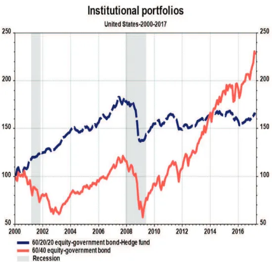
In practice, Ilmanen (2011) highlights that institutional practices have evolved from the traditional 60/40 equity/government bond split, i.e. 60% of the portfolio allocated to equities and 40% to fixed income securities (bonds), to globally diversified portfolios, often including emerging markets and alternative assets, which were seen as having almost no correlation with traditional stocks and bonds. Large institutional losses in 2008 raised significant questions about the best way to pursue asset allocation: Page and Taborsky (2011) showed that diversification does not accomplish its goals: diversification often disappears when most needed:

(11)

Figure 1: Traditional institutional portfolios (Author’s calculations)

To alleviate the difficulties encountered in the context of the Great Recession, this thesis proposes certain topics for reflection and discussion on the measures to be taken to truly diversify portfolios. The first one is to deepen the knowledge of interaction dynamics between financial markets the macroeconomy (Chapters 1 to 3). The second one is to explore a new way of capital allocation (Chapter 4).

With a view to a better understanding of the complex relationship between financial markets and the macroeconomy, a well-worked theory of macro-based asset allocation is introduced in the Chapter 1. The objective is to illustrate that asset returns are not correlated with the business cycle but are primarily caused by the economic cycles. To demonstrate this claim, economic cycles are first rigorously defined, namely the

(12)

classi-cal business cycle and the growth cycle, which is better known as the output gap. The description of different economic phases is refined by jointly considering both economic cycles. The theoretical influence of economic cycles on time-varying risk premiums is then explained based on two key economic concepts: nominal GDP and adaptive expec-tations. It is exhibited over the period from January 2002 to December 2013: dynamic investment strategies based on economic cycles turning points emphasize the importance of economical cycles, especially the growth cycle, for euro and dollar-based investors. An empirical analysis in the United States over the period from January 2002 to December 2013 highlight that this economic cyclical framework can improve strategic asset allocation choices.

In theory, dynamic macro-based regime-switching asset allocations achieve thus su-perior risk adjusted returns. Yet, economic turning points detection in real time is a notorious difficult task. One stylised fact of economic cycles is the non-linearity: the relationship between variables is not simply static and stable, but instead is dynamic and fluctuating. For example, Phillips (1958) concludes the last sentence of his first para-graph with: ”The relation between unemployment and the rate of change of wage rates is therefore likely to be highly non-linear”.

Real-time regime classification and turning points detection require thus methods ca-pable of taking into account the non-linearity of the cycles. In this respect, many para-metric models have been proposed, especially Markov switching models (see Piger (2011) for a review) and probit models (see Liu and Moench (2016) for a review). Parametric models are effective if the true data generating process (DGP) linking the observed data to the economic regime is known. In practice, however, one might lack such strong prior knowledge.

Non-parametric methods, such as machine-learning algorithms1_{, do not rely on a}

spec-ification of the DGP. The machine-learning approach assumes that the DGP is complex

1

Machine learning generally refers to the development of methods that optimize their performance iteratively by ”learning from the data”. Machine learning is broadly understood as a group of methods that analyse data and make useful discoveries and inferences from the data.

(13)

and unknown and attempts to learn the response by observing inputs and responses and finding dominant patterns. This places the emphasis on a model’s ability to predict well and focuses on what is being predicted and how prediction success should be measured2_.

Machine learning is used in spam filters, ad placement, credit scoring, fraud detection, stock trading, drug design, and many other applications, but it is largely unknown in economics (with the exception of Giusto and Piger (ming), Ng (2014) and Berge (2015)). The real-time ability of several machine learning algorithms (from very simple to quite complex) to nowcast economic turning points is gauged in Chapter 2 and Chapter 3. The aim is to quickly and accurately detect economic turning points in the United States and in the euro area.

In Chapter 3, probabilistic indicators are created from a simple and transparent su-pervised machine-learning algorithm known as Learning Vector Quantization (Kohonen (2001)). Those indicators are robust, interpretable and preserve economic consistency. In Chapter 3, a more complex approach is evaluated: ensemble machine learning algorithms, referred to as random forest (Breiman (2001)) and as boosting (Schapire (1990)), are ap-plied. The two key features of those algorithms are their abilities to entertain a large number of predictors and to perform estimation and variable selection simultaneously.

In both chapters, profit maximization measures are computed in addition to more standard criteria to assess the value of the models to take into account the disconnection between econometric predictability and actual profitability (see, among others, Cenesi-zoglu and Timmermann (2012) or Brown (2008)).

Importantly in this Thesis, when comparing predictive accuracy and profit measures, the model confidence set procedure proposed by Hansen et al. (2011) is applied to avoid

2

For prediction, the most common form of machine learning is supervised learning. Imagine that we want to build a system that can classify images as containing, say, a house, a car, a person or a pet. We first collect a large data set of images of houses, cars, people and pets, each labelled with its category. During training, the machine is shown an image and produces an output in the form of a vector of scores, one for each category. We want the desired category to have the highest score of all categories, but this is unlikely to happen before training. We compute an objective function that measures the error (or distance) between the output scores and the desired pattern of scores. The machine then modifies its internal adjustable parameters to reduce this error. These adjustable parameters, often called weights, are real numbers that can be seen as ”knobs” that define the input-output function of the machine.

(14)

data snooping. Data snooping occurs when a given set of data is used more than once for purposes of inference or model selection and leads to the possibility that any results obtained in a statistical study may simply be due to chance rather than to any merit inherent in the method yielding the results (White (2000))3_.

Both approaches are effective to detect economic turning points in real time over the period from January 2002 to December 2013. Strategies based on the turning points of the growth cycle induced by the models achieve thus excellent risk-adjusted returns in real time: timing the market is possible.

At last, modern and complex portfolio optimisation methods are optimal in-sample, but out-of-sample underperform alternative methods that are suboptimal in-sample. For instance, DeMiguel et al. (2009) demonstrate that the equal-weighted allocation, which gives the same importance to each assets, beats the entire set of commonly used portfolio optimization techniques.

L´opez de Prado (2016a) points out that these methods lack the notion of hierarchy, thereby allowing weights to vary freely in unintended ways. Indeed, Nobel prize laureate

Herbert Simon has demonstrated that complex systems can be arranged in a natural hierarchy, comprising nested sub-structures (Simon (1962)): ”the central theme that runs

through my remarks is that complexity frequently takes the form of hierarchy, and that hierarchic systems have some common proper-ties that are independent of their specific content. Hierarchy, I shall argue, is one of the central structural schemes that the architect of complexity uses”.

Building upon the fundamental notion of hierarchy, a hierarchical clustering based asset allocation method, which uses unsupervised machine learning techniques4_{, is}

in-3

Researchers conducting multiple tests on the same data tend to publish only those that pass a statistical significance test, hiding the rest. Because negative outcomes are not reported, readers are only exposed to a biased sample of outcomes. This problem, called ”selection bias”, is caused by multiple testing combined with partial reporting. It appears in many different forms: analysts who do not report the full extent of the experiments conducted (”file drawer effect”), journals that only publish ”positive” outcomes (”publication bias”), managers who only publish the history of their (so far) profitable strategies (”self selection bias”), etc. What all these phenomena have in common is that critical information is hidden from the decision maker, with the effect of a much larger than anticipated Type I Error probability.

4

(15)

troduced in Chapter 4. The out-of-sample performances of hierarchical clustering based portfolios and more traditional risk-based portfolios are evaluated across three disparate datasets, which differ in terms of number of assets and composition of the universe (”S&P sectors”, multi-assets and individual stocks). The empirical results indicate that hierarchi-cal clustering based portfolios are robust, truly diversified and achieve statistihierarchi-cally better risk-adjusted performances than commonly used portfolio optimization techniques.

The rest of the thesis proceeds as follows. Chapter 1 provides a clear, precise and efficient framework for macro-based investment decisions. Chapter 2 underlines that a very simple simple machine-learning algorithm known as Learning Vector Quantization appears very competitive with commonly used alternatives. Chapter 3 points out the interest of ensemble machine learning algorithms, referred to as random forest and as boosting. Chapter 4 presents the hierarchical clustering based asset allocation method.

(16)

(17)

Chapter 1 Time-varying risk premiums and

economic cycles

Abstract

Asset returns are not correlated with the business cycle but are primarily caused by the economic cycles. To validate this claim, economic cycles are first rigorously defined, namely the classical business cycle and the growth cycle, better known as the output gap. The description of different economic phases is refined by jointly considering both economic cycles. The theoretical influence of economic cycles on time-varying risk premiums is then explained based on two key economic concepts: nominal GDP and adaptive expectations. Simple dynamic investment strategies confirm the importance of economical cycles, especially the growth cycle, for euro and dollar-based investors. At last, this economic cyclical framework can improve strategic asset allocation choices.

(18)

Introduction

The willingness of investors to bear risk varies over time, larger in good times, and less in bad times, leading to time-varying risk premiums (Cochrane (2016)). Yet, there is still no consensus on the definition of good and bad time.

The most common approach is to consider the business cycle expansions and recessions (see, among others, Lustig and Verdelhan (2012)). Cooper and Priestley (2009) choose a slightly different way and point out the importance of the output gap for investment decisions. They note that the output gap is a classical business cycle variable that begins to fall before and throughout every recession. At last, some authors sometimes consider four distinct phases of the business cycle: ”expansion”, ”peak”, ”recession” and ”recovery ” (see, for example, Ahn et al. (2016)). The business cycle is thus a fundamental yet ambiguous concept, since it can refer to conceptually different economic fluctuation.

To deepen the knowledge of interaction dynamics between financial markets the macroe-conomy, this ambiguity needs above all to be removed. To this end, economic cycles are rigorously defined, namely the classical business cycle and the growth cycle, which seeks to represent the fluctuations around the trend. If we consider the trend growth rate as the potential growth rate, the growth cycle is better known as the output gap. The de-scription of different economic phases is then refined by jointly considering both economic cycles. It improves the classical analysis of economic cycles by considering sometimes two distinct phases and sometimes four distinct phases.

To explain the theoretical the influence of economic cycles on the time-varying risk premiums, the key concept is nominal growth expectations, which is the same thing as saying that income expectations are crucial. Indeed, a fall in nominal GDP growth tends to lead to mass unemployment, lower profits and sharply higher debt defaults (Keynes (1936) and Sumner (2014)). Forward-looking investors adjust thus their portfolios accord-ing to their ever-changaccord-ing current expectations of future events. The theory of adaptive expectations (Fisher (1911)) makes the link between the cyclical framework and

(19)

nomi-nal growth expectations. For example, when the real growth rate is above its potential, inflation pressures surge: the nominal growth rate of the economy increases. Adaptive expectations imply that nominal growth rate expectations should increase.

To gauge the potential value of this cyclical framework, dynamic investment strategies based on economic cycles turning points are created. Empirical results highlight the importance of economical cycles, especially the growth cycle, for euro and dollar-based investors. Indeed, strategies based on output gap turning points statistically outperform not only passive buy-and-hold benchmarks, but also business cycles’ strategies, in the United States and in the euro area.

In other words, asset prices and returns are not correlated with the business cycle (Cochrane (2016)) but are primarily caused by the economic cycles. Assessing if the current growth rate of the economy is above or under the trend growth rate is thus the most crucial task for investors.

At last, the presence of regimes with different correlations and assets’ characteristics can enhance strategic asset allocation, which is the most important determinant of long run investment success (Campbell and Viceira (2002)). Since correlations should theoret-ically vary during economic regimes, the main idea is to build a portfolio that would stay diversified when needed. Empirical results illustrate the influence of the correlation ma-trix on strategic asset allocation. In particular, investment-grade corporate bonds are not substitute to government bonds and risk-averse investors should select an asset allocation based on a correlation matrix whose elements are generated from bad times periods.

1.1 Cyclical framework

1.1.1 Economic cycles definitions

The classical business cycle definition is due to Burns and Mitchell (1946): ”Business

(20)

organize their work mainly in business enterprises: a cycle consists of expansions occur-ring at about the same time in many economic activities, followed by similarly general recessions, contractions, and revivals which merge into the expansion phase of the next cycle”. The business cycle is meant to reproduce the cycle of the global level of activity

of a country. The turning points of that cycle (named B for peaks and C for troughs) separate periods of recessions from periods of expansions.

Burns and Mitchell (1946) point out two main stylised facts of the economic cycle. The first is the co-movement among individual economic variables: most of macroeconomic time series evolve together along the cycle. The second is non-linearity: the effect of a shock depends on the rest of the economic environment. In other words, economic dynamics during economically stressful times are potentially different from normal times. For instance, small shock, such as a decrease in housing prices, can sometimes have large effects, such as recessions.

The growth cycle, introduced by Mintz (1974), seeks to represent the fluctuations of the GDP around its long-term trend. Mintz (1974) indicates that the rationale for investigating the growth cycle is that absolute prolonged declines in the level of economic activity tend to be rare events when the economy grows at a sustained and stable rate, so that in practice many economies do not very often exhibit recessions in classical terms. As a consequence, other approaches to produce information on economic fluctuations have to be proposed.

Growth cycle turning points (named A for peaks and D for troughs) have a clear meaning: peak A is reached when the growth rate decreases below the trend growth rate and the trough D is reached when the growth rate overpasses it again. Those downward and upward phases are respectively named slowdown and acceleration. A slowdown signals thus a prolonged period of subdued economic growth though not necessarily an absolute decline in economic activity. In other words, all recessions involve slowdowns, but not all slowdowns involve recessions.

(21)

If the long-term trend is considered as the estimated potential level1_{, then the growth}

cycle equals the output gap. A turning point of the output gap occurs when the current growth rate of the activity is above or below the potential growth rate, thereby signalling increasing or decreasing inflation pressures.

The ABCD approach (Anas and Ferrara (2004)) refines the description of different economic phases by jointly considering the classical business cycle and the growth cycle. Let us suppose that the current growth rate of the activity is above the trend growth rate (acceleration phase). The downward movement will first materialize when the growth rate will decrease below the trend growth rate (point A). If the slowdown gains in intensity, the growth rate could become negative enough to provoke a recession (point B). Eventually, the economy should start to recover and exits from the recession (point C). As the recovery strengthens, the growth rate should overpass its trend (point D). However, a slowdown will not automatically translate into a recession: if the slowdown is not severe enough to become a recession, then point A will not be followed by point B, but by point D.

This framework improves thus the classical analysis of economic cycles by allowing sometimes two distinct phases, if the slowdown is not severe enough to become a recession, and sometimes four distinct phases, if the growth rate of the economy becomes negative enough to provoke a recession.

1.1.2 Turning point chronology

A cycle turning point chronology is required for empirical studies to create and validate real-time detection and forecasting methods. The turning point chronology is only suitable for ex post explanatory analyses and not for ex ante decision making.

In the United States, the NBER’s Business Cycle Dating Bureau’s Committee deter-mines the peaks and troughs of the classical business cycle. In the euro area, the CEPR euro area Business Cycle Dating Committee establishes the chronology of recessions and

1

The potential output is the maximum amount of goods and services an economy can turn out at full capacity.

(22)

expansions. The European chronology is only available on a quarterly basis. To refine the chronology, the monthly GDP introduced by Raffinot (2007)2 _{is exploited in this article.}

For instance, the monthly GDP allows to select the month with the lowest level within the quarter selected by the CEPR to be chosen as the through of the recession.

If dating the classical business cycle is not an easy task, then dating the growth cycle is quite challenging since the series must first be de-trended. Several growth cycle extraction methods have been proposed in statistical literature, ranging from filtering techniques to parametric modelling, mainly based on state-space models and Markov switching models (see Anas et al. (2008) for a review). As advocated by Nilsson and Gyomai (2011), a double Hodrick-Prescott filter (18 months-96 months) is used on the monthly GDP3 _(see

Appendix 1.A for more information on this filter).

The turning points of the growth cycle are then estimated by the non-parametric procedure introduced by Harding and Pagan (2002). The algorithm first identifies peaks as observations that are lower over a two-sided window of five months and troughs are points associated with observations in the five month window that are higher. The algorithm then applies censoring rules to narrow the turning points of the reference cycle: the duration of a cycle must be no less than 15 months, while the phase (peak to trough or trough to peak) must be no less than 5 months.

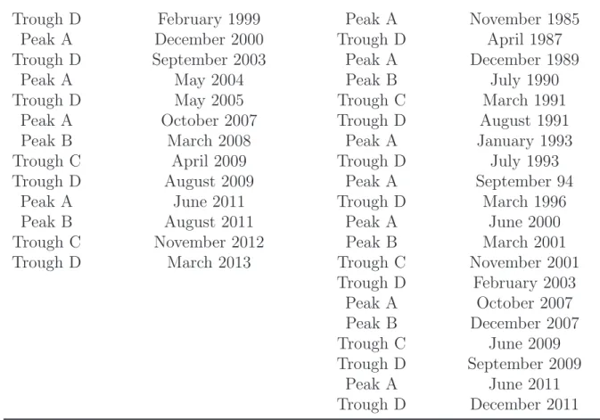
The complete chronology is contained in the table 1.14_{. The turning point chronology}

highlights the persistence of the regimes and the non-linearity of the cycles: the sequence of up and down phases is recurrent but not periodic. Expansions are longer than recessions. Moreover, even if the American and euro area chronologies are linked, they are quite distinct. For example, there was no double dip in the United States following the Great Recession and there was no recession in the euro area following the dot-com bubble burst.

2

A temporal disaggregation based on business surveys of the non revised values of gross domestic product GDP is used to develop a monthly indicator of GDP.

3

In unreported results, others filters were tested, such as Christiano and Fitzgerald (2003) and Baxter and King (1999). The empirical results are qualitatively similar.

4

The American chronology starts in 1985, since Stock and Watson (2003) demonstrate that approxi-mately 40% of 168 macro variables have significant breaks in their conditional variance during 1983-1985.

(23)

Table 1.1: Turning point chronology

Euro area (Jan 1999-December 2013) United States (Jan 1985-Dec 2013)

Trough D February 1999 Peak A November 1985 Peak A December 2000 Trough D April 1987 Trough D September 2003 Peak A December 1989

Peak A May 2004 Peak B July 1990 Trough D May 2005 Trough C March 1991

Peak A October 2007 Trough D August 1991 Peak B March 2008 Peak A January 1993 Trough C April 2009 Trough D July 1993 Trough D August 2009 Peak A September 94

Peak A June 2011 Trough D March 1996 Peak B August 2011 Peak A June 2000 Trough C November 2012 Peak B March 2001 Trough D March 2013 Trough C November 2001

Trough D February 2003 Peak A October 2007 Peak B December 2007 Trough C June 2009 Trough D September 2009 Peak A June 2011 Trough D December 2011

(24)

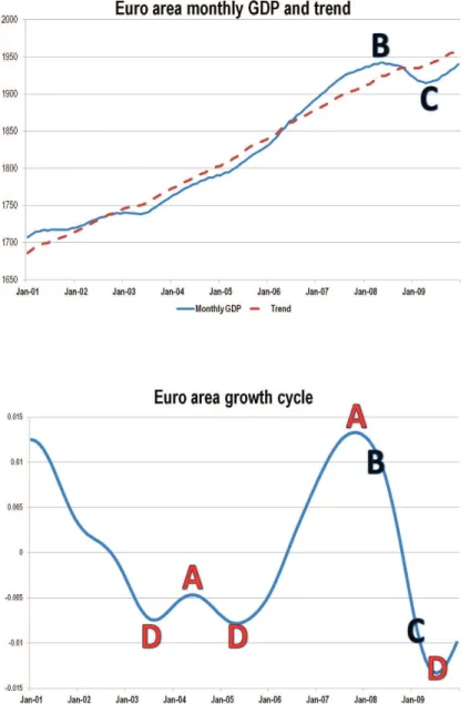
Figures 1.1 and 1.2 illustrate the monthly GDP, its trend, the growth cycle and exhibit the turning points in the euro area between 2001 and 2009. The euro area experienced a slowdown without recession in 2000-2003. In 2003, the recovery started to materialise (Point D), but the activity fell apart in May 2004 (Point A). The slowdown was short-lived: staring in May 2005 (point D) a building boom got under way. The slowdown starting in October 2007 (Point A) translated into the Great Recession a few months later (Point B). In April 2009, the recession was over (Point C).

Figure 1.1: Euro area monthly GDP and its trend over 2001-2009

(25)

1.2 Asset classes and economic cycles

1.2.1 The economic rationale

Key economic concepts

Two key basic economic concepts are needed to deepen the knowledge of interaction dynamics between financial markets the macroeconomy: nominal GDP and adaptive ex-pectations.

The economy is simply the sum of all transactions - the exchange of money and credit for goods, services, and financial assets - among individuals, banks, and governments. The technical term for the value of everything a country produces is nominal Gross Domestic Product (nominal GDP). It is total output (real GDP) times the current prices paid. Since all income is derived from production (including the production of services), the gross domestic income of a country should exactly equal its gross domestic product. Indeed, the gross domestic income is the total income received by all sectors of an economy within a State.

When nominal GDP falls, there is no longer enough spending to sustain the same number of jobs unless wages fall. Because wages are slow to adjust, unemployment rises instead (see Keynes (1936) and Sumner (2014)). Moreover, since most debts are not indexed to inflation, nominal income is the best measure of a person’s ability to repay their debts. When determining how much debt to take on, borrowers consider their ability to repay that debt. If income gains falls short of these expectations, interest and principal payments will be more burdensome than what was planned for. Problems of debt overhang become that much worse for the economy and debt defaults rise. To sump up, a fall in nominal GDP growth tends to lead to mass unemployment, lower profits and sharply higher debt defaults.

Adaptive expectation models are ways of predicting an agent’s behaviour based on their past experiences and past expectations for that same event. They are introduced by

(26)

(Fisher (1911)) and most famously used by Friedman (1957). For example, if consumers begin to actually see prices rising, they will begin to form robust expectations of inflation-ary expectations. The same theory might claim that consumers will expect an economic recovery to begin only after ample evidence that the turning point has been passed. The expectations-augmented Phillips curve introduces adaptive expectations into the Phillips curve. This equation appears in many recent New Keynesian dynamic stochastic general equilibrium models (Roberts (1995)).

Interactions between economic cycles and asset classes

The existing link between asset classes and the economy is not straightforward, especially for equities.

The stock price or the value of a company is the sum of all future dividend payments discounted to its present value. Under a constant payout ratio, the dividend growth rate will equate to the growth rate in earnings. In other words, investors buy a stock for its future earnings potential. Since the sum of all money earned in an economy each year is the nominal GDP, equity prices should thus be linked to nominal growth expectations (not real growth expectations). When the real growth rate is above its potential, inflation pressures surge: the nominal growth rate of the economy increases. Adaptive expectations imply that nominal growth rate expectations should increase, which is the same thing as saying that income expectations should rise5_{. In theory, equities should thus perform}

well during acceleration phases and suffer during slowdowns. Since slowdowns signal a prolonged period of subdued economic growth though not necessarily an absolute decline in economic activity, equities performances can thus be negative when real growth rate are positive.

In theory, government bonds should perform well during slowdowns and recessions. Indeed, the expectations theory of the term structure holds that the long-term interest

5

A link with the classical drivers of the equity risk premium can be done. For example, market participants’ expectations about the future economic activity affect the determination of dividends and thus stock return premiums.

(27)

rate is a weighted average of present and expected future short-term interest rates plus a term premium (the latter captures the compensation that investors require for bearing interest rate risk). If the growth rate of the activity is lower than the potential growth rate, inflation pressures trend down and the central bank is more likely to cut rates. In consequence, investors should forecast a lower path of future short-term interest rates. Long-term rates should thus decrease (and bond prices increase).

Because a company’s capacity to service its debt is uncertain, corporate bond should offer a higher expected return compared to sovereign bonds. Corporate bonds can thus be decomposed as the sum of a government bond plus a spread, which compensates for the expected losses due to default. The probability of default for an investment grade firm is quite small, but raises when corporate income expectations decline. Investment grade bonds should benefit from falling rates during slowdowns, but to a lesser extent that government bonds. During acceleration and expansion, investment grade bonds should take advantage of the declining spread and the coupon. High-yield bonds should behave more like equities, since defaults have always been commonplace.

For all assets, volatility is higher during bad times. One plausible explanation is that the uncertainty around the likely course of monetary policy rises during bad times, leading to an increase in the volatility of the safest and riskiest assets.

1.2.2 Historical facts

Table 1.2 details the four asset classes in consideration. The investment universe is as stripped-down and simple as possible without raising concerns that the key results will not carry over to more general and intricate asset classes or factors.

(28)

Table 1.2: Asset classes

Asset class Index

Equities Euro area Euro Stoxx 50 (total return) United States S&P 500 (total return)

Government bonds Euro area_{United States BOFA Merrill Lynch Treasury Master Index (total return)}IBOXX SOVEREIGNS EUROZONE ALL MATS (total return) Invesment Grade bonds Euro area IBOXX Euro Corp All Mats (total return)

United States Barclays Capital U.S. Corporate Investment Grade Index (total return) High-yield bonds Euro area_{United States BOFA Merrill Lynch High Yield 100 Index (total return)}IBOXX EUR High Yield Index (total return)

All series are provided by Datastream.

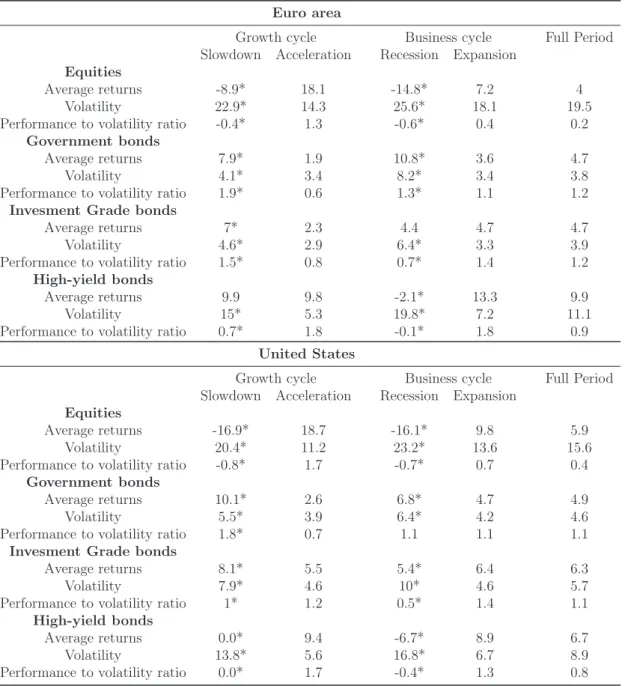
Table 1.3 confirms that asset classes perform differently during different stages of both economic cycles and no single asset class dominate under all economic conditions, in line with the theory.

The returns of the riskiest assets, equities and high yield bonds, are pro-cyclical and contrasted. For instance, in the United States, equities increase at a rate of 18.7% dur-ing expansions, whereas they fall by almost 17% durdur-ing slowdowns. The amplitude of expected returns equals thus 35%.

The expected returns of government bonds and investment grade bonds are always positive, even if they are more attractive during bad times. For example, in the euro area, the performance of government bonds is four time higher during slowdowns (7.9%) than during expansions (1.9%).

Moreover, the presence of asymmetric volatility for risky assets is most apparent during bad times (slowdowns) and very bad times (recessions) when a large decline in stock prices or high yield prices is associated with a significant increase in market volatility. For example, in the euro area, the stock market volatility increases from 14.3% during accelerations to 22.9% during slowdowns.

In the euro area, the performance of high yield bonds is surprisingly the same during accelerations and slowdowns. This is not in line with the theory and with the results observed in the United States. The limited size of this market and the short sample period may partly explain this anomaly.

(29)

of an investment to the amount of risk undertaken to capture these returns, is statistically different at a 95% confidence level in each macroeconomic environment (except for the American government bonds as regards the business cycle).

1.3 Dynamic investment strategies

1.3.1 Active portfolio management and economic cycles

To study time-varying risk premiums, the traditional approach is to test whether assets excess returns are predictable. The literature on return predictability is voluminous (see, for example, Rapach et al. (2013) for a review on stocks returns, Zhou and Zhu (2017) for government bonds returns and Lin et al. (2016) for corporate bonds returns). One drawback with this approach is the disconnection between econometric predictability and actual profitability (see, among others, Cenesizoglu and Timmermann (2012) or Brown (2008)). This paper only focusses on profitability6_.

To examine the economic value of market forecasts, the current practice is to calculate realized utility gains for a mean-variance investor who optimally allocates across equities (or bonds or corporate bonds) and the risk-free asset on a real-time basis. Portfolio weights are usually constraint to lie between -50% and 150% each month.

Another approach has been preferred, mainly for two reasons. First, the mean-variance optimisation requires the investor to forecast the excess returns and the variance of as-set returns.But, even small estimation errors can result in large deviations from optimal allocations in an optimizer’s result (Michaud (1989)). This is why, academics and practi-tioners have developed risk-based portfolio optimization techniques (minimum variance, equal risk contribution, risk budgeting,...), which do not rely on return forecasts (Roncalli (2013)). Yet, even the variance is hard to estimate. A ten-year rolling window or five-year

6

To test the predictability of the proposed economic framework, a regression between asset returns and the evolution of the output gap should be done. The evolution of the output gap exhibits if the current growth rate of the economy is above the trend or not. It differs from Cooper and Priestley (2009) because the sign and the magnitude of the output gap are not taken into account.

(30)

Table 1.3: Summary of returns and risk measures in each macroeconomic en-vironment, 1999-2013

Euro area

Growth cycle Business cycle Full Period Slowdown Acceleration Recession Expansion

Equities

Average returns -8.9* 18.1 -14.8* 7.2 4

Volatility 22.9* 14.3 25.6* 18.1 19.5

Performance to volatility ratio -0.4* 1.3 -0.6* 0.4 0.2 Government bonds

Average returns 7.9* 1.9 10.8* 3.6 4.7

Volatility 4.1* 3.4 8.2* 3.4 3.8

Performance to volatility ratio 1.9* 0.6 1.3* 1.1 1.2 Invesment Grade bonds

Average returns 7* 2.3 4.4 4.7 4.7

Volatility 4.6* 2.9 6.4* 3.3 3.9

Performance to volatility ratio 1.5* 0.8 0.7* 1.4 1.2 High-yield bonds

Average returns 9.9 9.8 -2.1* 13.3 9.9

Volatility 15* 5.3 19.8* 7.2 11.1

Performance to volatility ratio 0.7* 1.8 -0.1* 1.8 0.9 United States

Growth cycle Business cycle Full Period Slowdown Acceleration Recession Expansion

Equities

Average returns -16.9* 18.7 -16.1* 9.8 5.9

Volatility 20.4* 11.2 23.2* 13.6 15.6

Performance to volatility ratio -0.8* 1.7 -0.7* 0.7 0.4 Government bonds

Average returns 10.1* 2.6 6.8* 4.7 4.9

Volatility 5.5* 3.9 6.4* 4.2 4.6

Performance to volatility ratio 1.8* 0.7 1.1 1.1 1.1 Invesment Grade bonds

Average returns 8.1* 5.5 5.4* 6.4 6.3

Volatility 7.9* 4.6 10* 4.6 5.7

Performance to volatility ratio 1* 1.2 0.5* 1.4 1.1 High-yield bonds

Average returns 0.0* 9.4 -6.7* 8.9 6.7

Volatility 13.8* 5.6 16.8* 6.7 8.9

Performance to volatility ratio 0.0* 1.7 -0.4* 1.3 0.8

Note: This table reports annualized average monthly returns, annualized standard deviation (volatility) and performance to volatility ratio of asset classes during different economic regimes over the period 1999-2013. The performance to volatility ratio compares the expected returns of an investment to the amount of risk undertaken to capture these returns, the higher the better. * signals that the null hypothesis of equal mean of the Wilcoxon rank sum is rejected at a 95% confidence level.

(31)

rolling window is often applied to estimate the variance. In a regime switching framework, another solution has to be found.

Second, the relative profitability of a dynamic strategy using econometrically superior forecasts shrinks significantly if the investor is highly risk averse and heavily constrained (Baltas and Karyampas (2016)). As a matter of fact, investors typically face a number of constraints, either by mandate or regulation, which put hard thresholds on minimum and maximum allocation across risky assets. For instance, by law in France, equity funds managers must have at least 60% of their portfolio invested in equities.

To address the same problem with another approach, simple hypothetical dynamic trading strategies are created7_{. Dynamic strategies should take advantage of positive}

economic regimes, as well as withstand adverse economic regimes and reduce potential drawdowns.

We consider an investor managing a portfolio consisting of an unique asset class (either stocks or government bonds) investing 100 e or 100$ on January 1, 1999. Each month the investor decides upon the fraction of wealth to be invested based on the current state of the economy. If the asset class should perform well, then the investor can leverage his portfolio (120% of his wealth is invested on the asset and 20% of cash is borrowed), otherwise he only invests 80% of his wealth and 20% is kept in cash. The active strategies are then compared among them and with the buy-and-hold strategy - henceforth a passive strategy. These strategies are named 120/80 hereafter8_.

To avoid look-ahead bias, the reallocation takes place at the beginning of the month following the turning point. As a matter of fact, an investor could not know at the beginning of any month whether a turning point would occur in that month.

In contrast to the standard approach, asset returns are not predicted but only

condi-7

These strategies reflects the investment process in place in the asset management companies where I used to work.

8

Since asset classes perform differently during different stages of the growth cycle, it might be reason-able to rebalance the portfolio (shifting allocation weights) based on the stage of the economic cycles. For brevity reasons, the results of such strategies are not presented. Yet if the 120/80 strategies work for both bonds and equities, it seems reasonable to conclude that dynamic asset allocation strategies should perform well.

(32)

tioned on the stage of the economic cycle.

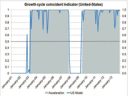
The main weakness is that the strategies described so far are not implementable be-cause investors do not know turning point dates in real time. Yet, recent academic studies such as Ng (2014) and Berge (2015) apply a machine learning algorithm referred to as boosting ((Schapire (1990))) to the problem of identifying business cycle turning points in the United States. Even if forecasting turning points remains challenging, they conclude that nowcasting turning points in real time is feasible.

1.3.2 Comparison criteria

Performance and risk measures

To compare the different strategies, four different performance and risk measures are computed:

• The annualized average returns (µ)

• The annualized standard deviation (Volatility)(σ)

• The certainty-equivalent return (CEQ) is the risk-free rate of return that the investor is willing to accept instead of undertaking the risky portfolio strategy.

CEQ = (µ − rf) −

γ 2σ

2

where rf is the risk-free rate9 and γ is the risk aversion. Results are reported for the

case of γ = 1; 3; 5. More precisely, the CEQ captures the level of expected utility of a mean-variance investor, which is approximately equal to the certainty-equivalent return for an investor with quadratic utility (DeMiguel et al. (2009)).

• The Max drawdown (MDD) is an indicator of permanent loss of capital. It measures the largest single drop from peak to bottom in the value of a portfolio. In brief, the MDD offers investors a worst case scenario.

9

(33)

Pesaran and Timmermann (1994) and Han et al. (2013) demonstrate that the total cost of transactions appears to be low, less than 1% (around 50 basis points when trading in stocks while the cost for bonds is 10 basis points). To simplify, since economic turning points are rare, no transaction costs are considered.

Data snooping

To avoid data snooping, which occurs when a given set of data is used more than once for purposes of inference or model selection (White (2000)), the model confidence set (MCS) procedure proposed by Hansen et al. (2011) is computed.

The MCS procedure is a model selection algorithm, which filters a set of models from a given entirety of models. The resulting set contains the best models with a probability that is no less than 1 − α with α being the size of the test.

An advantage of the test is that it not necessarily selects a single model, instead it acknowledges possible limitations in the data since the number of models in the set containing the best model will depend on how informative the data are.

More formally, define a set M0 that contains the set of models under evaluation indexed

by: i = 0, ..., m0. Let di,j,t denote the loss differential between two models by

di,j,t = Li,t− Lj,t, ∀i, j ∈ M0

L is the loss calculated from some loss function for each evaluation point t = 1, ..., T . The set of superior models is defined as:

M∗ _{= {i ∈ M}0 : E[di,j,t] ≤ 0 ∀j ∈ M0}

The MCS uses a sequential testing procedure to determine M∗_{. The null hypothesis}

(34)

    

H0,M : E[di,j,t] = 0 ∀i, j ∈ M where M is a subset of M0

HA,M : E[di,j,t] 6= 0 for some i, j ∈ M

When the equivalence test rejects the null hypothesis, at least one model in the set M is considered inferior and the model that contributes the most to the rejection of the null is eliminated from the set M . This procedure is repeated until the null is accepted and the remaining models in M now equal cM∗

1−α.

According to Hansen et al. (2011), the following two statistics can be used for the sequential testing of the null hypothesis:

ti,j = di,j q d var(di,j) and ti = di q d var(di)

where m is the number of models in M , di = (m − 1)−1

P

j∈Mdi,j, is the simple

loss of the ith _{model relative to the averages losses across models in the set M , and}

di,j = (m)−1Pm_t=1di,j,t measures the relative sample loss between the ith and ith models.

Since the distribution of the test statistic depends on unknown parameters a bootstrap procedure is used to estimate the distribution.

In this paper, the MCS is applied with a profit maximization loss function (CEQ). As regards investment strategies, the MCS aims at finding the best model and all models which are indistinguishable from the best, not those better than the benchmark. To determined if models are better than the benchmark, the stepwise test of multiple reality check by Romano and Wolf (2005) and the stepwise multiple superior predictive ability test by Hsu et al. (2013) should be considered. However, if the benchmark is not selected in the best models set, investors can conclude that their strategies ”beat” the benchmark.

(35)

1.3.3 Empirical results

Tables 1.4 and 1.5 highlight that active investment strategies based on the growth cycle statistically outperform not only passive buy-and-hold benchmarks, but also business cycles’ strategies, in the United States and in the euro area.

For both government bonds and equities, strategies based on growth cycle turning points are always the only constituent of the best models set cM∗

75%, whatever the degree

of risk aversion.

In comparison with the benchmark, 120/80 equities strategies based on output gap turning points reduce the volatility and the losses in extreme negative events (MDD). For instance, the MDD decreases from 59.9% to 52.4% in the euro area and from 50.9% to 43% in the United States. To sum up, strategies based on the growth cycle improve the returns and reduce risk measures.

As regards governments bonds, 120/80 strategies based on the growth cycle improve returns while taking almost the same risk. In the euro area, the MDD declines from 5.7% to 5.2%, whereas the MDD slightly increases from 4.8% to 5% in the Unites States.

The business cycles’ strategies produced mixed results. In particular, for bond in-vestors, they do not add any value and the CEQ of the strategy is lower than the CEQ of the benchmark for all the degrees of risk aversion. As regards equities, avoiding the worst times is undoubtedly a good idea to get better returns, especially in the United States. The performance progresses from 4% to 5.4% in the euro area and from 5.9% to 8.3% in the United States. Yet risk measures increase. In particular,, the MDD surge from 59.9% to 65.4% in the euro area and the volatility rises from 15.5% to 16.8% in the United States.

In the end, expansions, which are composed of both acceleration and slowdown periods, can not be considered as good times, especially for the safest assets. The only suitable definition of good and bad times is thus acceleration and slowdown periods.

(36)

Table 1.4: Equities: 120/80 investment strategies

Euro area

Growth cycle 120/80 Business cycle 120/80 Full period

Average returns 6.8 5.4 4.0 Volatility 18.0 21.5 19.5 CEQ : γ = 1 0.052* 0.031 0.021 CEQ : γ = 3 0.019* -0.015 -0.017 CEQ : γ = 5 -0.013* -0.062 -0.055 MDD -52.4 -65.4 -59.9 United States

Average returns 9.7 8.3 5.9 Volatility 15.1 16.8 15.5 CEQ : γ = 1 0.086* 0.069 0.047 CEQ : γ = 3 0.063* 0.041 0.023 CEQ : γ = 5 0.040* 0.012 -0.001 MDD -43.0 -51.0 -50.9

Note: This table reports the characteristics of active strategies based on the state of the economic cycle over the period from January 1999 to December 2013. A 120/80 equity strategy is computed. Returns are monthly and annualized. The volatility corresponds to the annualized standard deviation. The certainty-equivalent return (CEQ) is the risk-free rate of return that the investor is willing to accept instead of undertaking the risky portfolio strategy. The Max drawdown (MDD) measures the largest single drop from peak to bottom in the value of a portfolio. * indicates the model is in the set of best models cM∗

75%.

Table 1.5: Government bonds: 120/80 investment strategies

Euro area

Average returns 5.2 4.4 4.7 Volatility 4.0 3.6 3.8 CEQ : γ = 1 0.051* 0.043 0.046 CEQ : γ = 3 0.050* 0.042 0.045 CEQ : γ = 5 0.048* 0.041 0.043 MDD -5.2 -5.2 -5.7 United States

Average returns 5.2 4.3 4.9 Volatility 4.8 4.4 4.6 CEQ : γ = 1 0.051* 0.042 0.048 CEQ : γ = 3 0.049* 0.040 0.046 CEQ : γ = 5 0.046* 0.038 0.044 MDD -5.0 -5.4 -4.8

Note: This table reports the characteristics of active strategies based on the state of the economic cycle over the period from January 1999 to December 2013. A 120/80 bond strategy is computed. Returns are monthly and annualized. The volatility corresponds to the annualized standard deviation. The certainty-equivalent return (CEQ) is the risk-free rate of return that the investor is willing to accept instead of undertaking the risky portfolio strategy. The Max drawdown (MDD) measures the largest single drop from peak to bottom in the value of a portfolio. * indicates the model is in the set of best models cM∗

75%.

These results have also implications for the risk management and hedging. Especially, in the options market one can utilize the current state of the economy to hedge the portfolio against the possible price declines. For example, besides following one of the

(37)

the previous strategy, writing an out-of-money covered call or buy a put option when the stock market is expected to decrease (slowdown or recession) would limit the losses.

Timing of turning point detection

A cyclical framework with learning gives content to the idea of an economy moving grad-ually from one regime to another, particularly if the central bank as well as the public is assumed to be updating its beliefs (Bernanke (2007)).

It implies that the strategies described in the previous sections should not rely on an exact timing of turning points detection. To verify the validity of this claim, the 120/80 strategies are computed based on different timings of the turning points detection: up to three months in advance, right in time or up to three months late.

Tables 1.6 and 1.7 illustrate that timing is an important issue, but an exact timing is not needed.

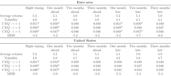
Table 1.6: Government bonds: 120/80 investment strategies and timing of growth cycle turning points detection

Euro area

Right timing One month Two months Three months One month Two months Three months ahead ahead ahead late late late Average returns 5.2 5.1 5.0 5.0 5.2 5.1 5.0 Volatility 4.0 4.0 4.0 4.0 4.1 4.1 4.1 CEQ : γ = 1 0.051* 0.050* 0.049 0.049 0.051* 0.050* 0.049 CEQ : γ = 3 0.050* 0.049* 0.048 0.048 0.049* 0.048 0.047 CEQ : γ = 5 0.048* 0.047* 0.046 0.046 0.048* 0.047* 0.046 MDD -5.2 -5.2 -5.2 -5.2 -5.2 -5.7 -6.0 United States

Right timing One month Two months Three months One month Two months Three months ahead ahead ahead late late late Average returns 5.2 5.3 5.1 5.1 5.1 5.0 4.9 Volatility 4.8 4.8 4.7 4.8 4.8 4.8 4.7 CEQ : γ = 1 0.051* 0.052* 0.050 0.050 0.050 0.049 0.048 CEQ : γ = 3 0.049* 0.050* 0.048 0.048 0.048 0.047 0.046 CEQ : γ = 5 0.046* 0.047* 0.045 0.045 0.045 0.044 0.045 MDD -5.0 -5.0 -5.0 -5.0 -5.3 -5.4 -5.4

Note: This table reports the characteristics of the active strategies based on different timing of the turning point detection: in advance, right in time or late. It is an in-sample analysis. A 120/80 equity strategy and a 120/80 bond strategy are computed. Returns are monthly and annualized. Active strategies are then compared with the buy-and-hold strategy. The volatility corresponds to the annualized standard deviation. The certainty-equivalent return (CEQ) is the risk-free rate of return that the investor is willing to accept instead of undertaking the risky portfolio strategy. The Max drawdown (MDD) measures the largest single drop from peak to bottom in the value of a portfolio. * indicates the model is in the set of best models cM∗

(38)

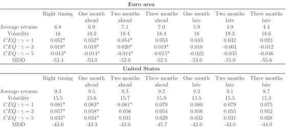
Table 1.7: Equities: 120/80 investment strategies and timing of growth cycle turning points detection

Euro area

Right timing One month Two months Three months One month Two months Three months ahead ahead ahead late late late Average returns 6.8 6.9 7.1 7.0 5.9 4.9 4.4 Volatility 18 18.2 18.4 18.4 18 18.3 18.6 CEQ : γ = 1 0.052* 0.052* 0.054* 0.053 0.043 0.032 0.023 CEQ : γ = 3 0.019* 0.019* 0.020* 0.019* 0.010 -0.001 -0.012 CEQ : γ = 5 -0.013* -0.014* -0.014* -0.015* -0.022 -0.035 -0.046 MDD -52.4 -53.0 -52.0 -52.5 -53.0 -55.0 -55.6 United States

Right timing One month Two months Three months One month Two months Three months ahead ahead ahead late late late Average returns 9.3 9.5 9.3 9.2 9.2 9.1 8.7 Volatility 15.5 15.6 15.7 15.9 15.5 15.5 15.3 CEQ : γ = 1 0.081* 0.083* 0.081* 0.079 0.080 0.079 0.075 CEQ : γ = 3 0.057* 0.058* 0.056 0.054 0.056 0.055 0.052 CEQ : γ = 5 0.033* 0.034* 0.031 0.029 0.032 0.031 0.028 MDD -43.0 -43.3 -43.0 -45.7 -43.0 -43.0 -44.0

Note: This table reports the characteristics of the active strategies based on different timing of the turning point detection: in advance, right in time or late. It is an in-sample analysis. A 120/80 equity strategy and a 120/80 bond strategy are computed. Returns are monthly and annualized. Active strategies are then compared with the buy-and-hold strategy. The volatility corresponds to the annualized standard deviation. The certainty-equivalent return (CEQ) is the risk-free rate of return that the investor is willing to accept instead of undertaking the risky portfolio strategy. The Max drawdown (MDD) measures the largest single drop from peak to bottom in the value of a portfolio. * indicates the model is in the set of best models cM∗

75%.

Table 1.6 highlights that bonds investors should rebalance their portfolio around the turning points or a month sooner in the United States and around the turning points or little bit later in the euro area. In the United States, the strategies ”right in time” and ”one month ahead” compose the best models sets cM∗

75% for all the degrees of risk aversion.

In the euro area, the best models sets cM∗

75% consist of many strategies and differ

depending on the degree of risk aversion. Yet, the strategies: ”right in time”, ”one month ahead”, ”one month late” and ”two months late” belong to all best models sets. These results are in line with the fact that markets forecast a monetary tightening only when there are inflation pressures: the current growth rate of the economy has to be above its potential.

Table 1.7 paints a contrasted picture. The behaviour of the investor differ depending on the country. In the United States, for all the degrees of risk aversion, the strategies ”right in time” and ”one month ahead” form the best models set cM∗

75%. In the euro area,

investors should shift weights in advance of the turning points: the strategy ”three months ahead” belongs to all best models set cM∗

75%. This result may stem from the leading role

(39)

To validate this claim, the same 120/80 investment strategy is tested on European equities, but the rebalancing of investments is based on American turning points instead of European turning points. Table 1.8 highlights that the 120/80 strategy based on the American cycle achieves higher returns (8.8% against 6.8%) than the one based on euro area cycle and is the only strategy in the best models set cM∗

75%. Euro-based equity

investors should thus focus on the American chronology instead of their own cycle. Table 1.8: European equities: 120/80 investment strategies based on the Amer-ican chronology

Euro area

European Growth cycle 120/80 American Growth cycle 120/80 Full period

Average returns 6.8 8.8 4.0 Volatility 18.0 19.1 19.5 CEQ : γ = 1 0.052 0.070* 0.021 CEQ : γ = 3 0.019 -0.033* -0.017 CEQ : γ = 5 -0.013 -0.003* -0.055 MDD -52.4 -52.2 -59.9

Note: This table reports the characteristics of active strategies based on the state of the economic cycle over the period from January 1999 to December 2013. A 120/80 equity strategy is computed. Returns are monthly and annualized. The volatility corresponds to the annualized standard deviation. The certainty-equivalent return (CEQ) is the risk-free rate of return that the investor is willing to accept instead of undertaking the risky portfolio strategy. The Max drawdown (MDD) measures the largest single drop from peak to bottom in the value of a portfolio. * indicates the model is in the set of best models cM∗

75%.

1.4 Strategic asset allocation and economic cycles

The primary goal of a strategic asset allocation is to create an asset mix which will provide an optimal balance between expected risk and return for a long-term investment horizon. Strategic asset allocation is the most important determinant of long run investment success (Campbell and Viceira (2002).

The asset allocation basis is to combine assets with low correlations to reduce the variance, or riskiness, of a portfolio. It is said to be the only the ”only free lunch” in investing (Markowitz (1952)). The traditional inputs required for an optimizer are expected returns, volatility and a correlation matrix. Even with more modern techniques, such as risk-based portfolio (Roncalli (2013)) or ”Hierarchical Risk Parity” (L´opez de Prado (2016a)), a correlation matrix is still needed.

(40)

1.4.1 Correlations and economic cycles

Tables 1.9 and 1.10 highlight that correlations are time varying and sensitive to economic cycles. In particular, asset classes are more correlated during bad times than during good times. We recall that bad times refer to slowdown periods (and thus recessions) and good times refer to acceleration periods. Expansions can not be considered as good times, since they are composed of both acceleration and slowdown periods.

An important implication of higher correlation is that otherwise-diversified portfolio lose some of diversification benefit during bad times, when most needed.

The correlation between stocks and bonds is arguably the most important correlation input to the asset allocation decision. The full sample average of the realized correlation is -0.14 in the euro area and -0.04 in the United States, but there has been substantial variation around this mean. From a theoretical point of view, equities should suffer during bad times and bonds should perform well. The correlation should be negative.

Good times are more complex to analyse. Equities should increase. Government bonds should benefit from the reinvestment of the coupons. Indeed, during good times, government interest rates should be high and coupons should support the performance of this asset10_.

The correlation between equities and government bonds should thus be slightly posi-tive, especially near the end of an acceleration period. Tables 1.9 and 1.10 confirm this assessment: the realized correlation during acceleration periods is 0.01 in the euro area and 0.05 in the United States.

The covariation between equities and credit bonds is also a crucial input to managing the risk of diversified portfolios. For instance, if credit appears attractive relative to equities, portfolio managers may choose to take a kind of equity risk via credit bonds.

Tables 1.9 and 1.10 emphasize that equities and credit bonds are more correlated

10

Low interest rates are not the symbol of easy monetary policy, but rather an outcome of excessively tight monetary policy (see Friedman (1992) and Friedman (1997)). If monetary conditions are tight then inflation and growth expectations decrease and as a consequence bond yields will also fall.

(41)

during bad times than during good times. For instance, in the euro area, there is a marked increase from -0.04 to 0.67 in the correlation between equities and investment grade bonds bonds during recessions. In the United States, the correlation between equi-ties and investment grade bonds is much more significant during slowdowns (0.63) than during accelerations (0.30). From a theoretical point of view, Merton (1974) posits that equity should behave like a call option on the assets of the firm, whereas risky debt should behave like a government bond plus a short position in a put option on the firm’s assets. The short option position embedded in credit bonds leads to negative convexity in their payoff profile. As a result, the relationship between credit and equity returns becomes stronger in the Merton model when firm and equity valuations fall.

As a consequence, investment-grade corporate bonds are not substitute to government bonds. Indeed, correlation to equities during bad times should be positive for investment-grade corporate bonds and negative for government bonds. The increasing importance of investment-grade corporate bonds in large institutional portfolios (Ilmanen (2011)) may partly explains the large losses during the last crisis.

Table 1.9: Return correlations in the euro area, 1999-2013 Eurostoxx Gov IG Eurostoxx Gov -0.14 IG 0.35 0.55 HY 0.62 -0.08 0.62 Acceleration Eurostoxx Gov IG Eurostoxx Gov 0.01 IG 0.09 0.83 HY 0.55 0.21 0.53 Slowdown Eurostoxx Gov IG Eurostoxx Gov -0.18 IG 0.48 0.42 HY 0.66 -0.18 0.66

(42)

Expansion Eurostoxx Gov IG Eurostoxx Gov -0.12 IG 0.08 0.73 HY 0.55 0.04 0.56 Recession Eurostoxx Gov IG Eurostoxx Gov -0.08 IG 0.67 0.38 HY 0.69 -0.14 0.69

(43)

Table 1.10: Return correlations in the United States, 1988-2013 S&P500 Gov IG S&P500 Gov -0.04 IG 0.32 0.73 HY 0.57 -0.02 0.48 Acceleration S&P500 Gov IG S&P500 Gov 0.05 IG 0.30 0.86 HY 0.53 0.09 0.45 Slowdown S&P500 Gov IG S&P500 Gov -0.10 IG 0.39 0.53 HY 0.63 -0.10 0.54 Expansion S&P500 Gov IG S&P500 Gov -0.02 IG 0.25 0.86 HY 0.51 0.06 0.42 Recession S&P500 Gov IG S&P500 Gov -0.10 IG 0.51 0.34 HY 0.70 -0.20 0.61

1.4.2 A truly diversified strategic asset allocation

Since correlations vary during economic regimes, the main idea is to build a portfolio that would stay diversified when needed. Indeed, assets correlations are a key input and nothing prevents from carefully selecting the correlation matrix used to establish the asset allocation. Only a chronology of the regimes is needed.

An out-of-sample analysis in the United States illustrates this important point (there is no recession in our sample before 2007 in the euro area, thereby drastically limiting an out-of-sample analysis).

Three different strategic asset allocations are computed. Only the correlation matrix used to estimate the weights differs. The first correlation matrix is calculated over the complete period 1988-2002. The second is calculated over the months labelled as slowdown

(44)

during the period 1988-2002. The third is calculated over the months labelled as recession during the period 1988-2002.

While respecting the chosen asset allocation, the three portfolios evolve from January 2003 to December 2013.

The investment universe is composed of the following assets: cash (Fed funds), S&P500, governments bonds, investment grade bonds and high-yield bonds.

The chosen targeted volatilities equal 6%, for risk adversed investors, and 10%, which is comparable to the historical volatility of the classical 60/40 asset allocation over the period 1988-2002.

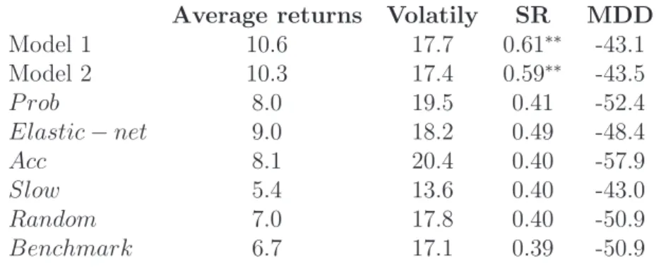
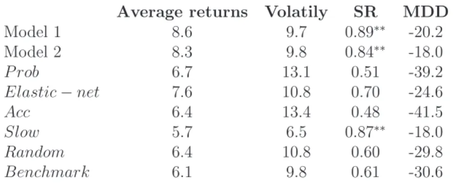
Tables 1.11 and 1.12 confirm the importance of the correlation matrix for asset al-location choices. In comparison with the benchmark, alal-locations based on slowdown or recession matrix reduce the out-of-sample volatility and the losses in extreme negative events (MDD). This is what risk-averse investors value the most.

For instance, considering the worst times (recessions) to build the correlation matrix, allows to reduce the MDD from 18.8% to 17.5% for a targeted volatility of 6% and from 42.0% to 37.6% for a targeted volatility of 10%.

Moreover, for all the degrees of risk aversion and all the targeted volatilities, the strate-gies based on the slowdown matrix are selected in the best models sets cM∗

75%. Strategies

based on the recession matrix are selected in all best models sets cM∗

75% but one. These

results confirm the interest of this approach. The strategy based on the full period matrix is only selected in one best models sets cM∗

75%, for a targeted volatility of 10% and γ = 1.

This strategy achieves higher returns (8.9%) but the volatility is higher than 10% and equals 11.8%, which is not in line with the initial objective.

To sum up briefly, investors should favour asset allocations based on bad times corre-lation matrix, since the portfolios stay diversified when needed.