Discovering different patterns inside SubSaharan countries defining more homogeneous clusters to simulate specific trade policies

1

This project is funded by the European Union under the 7th Research Framework Programme (theme SSH) Grant agreement nr 290752. The views expressed in this press release do not necessarily reflect the views of the European Commission.

Working Paper n°10

Discovering different patterns inside

Sub-Saharan countries defining more

homogeneous clusters to simulate specific

trade policies

Rafael de Arce, Saul de Vicente, Ramón Mahía, Eva Medina

UAM

Enhancing Knowledge for Renewed Policies against Poverty

Framework Program 7 Grant Agreement no.: 290752

Project Acronym: NO-POOR

Enhancing Knowledge for Renewed Policies against Poverty

Instrument: Collaborative Project Theme:

SSH-2011.4.1-1: TACKLING POVERTY IN A DEVELOPMENT CONTEXT

Working Paper

DISCOVERING DIFFERENT PATTERNS INSIDE SUB-SAHARAN

COUNTRIES: DEFINING MORE HOMOGENEOUS CLUSTERS TO

SIMULATE SPECIFIC TRADE POLICIES

TASK 5.1. HOW TRADE GLOBALISATON AFFECTS POVERTY July, 2014

(11 / 11 / 2013)

Project Coordinator: Prof. Xavier OUDIN Work Package 5 Leader Organisation: F-UFRJ Authors (alphabetical order): Prof. Dr. Rafael de Arce UAM

Mr. Saul de Vicente UAM Prof. Dr. Ramón Mahía UAM Prof. Dr. Eva Medina, UAM Miss Anda David UAM-IRD , Madrid, Spain

INDEX

1. INTRODUCTION ... 4

2. LITERATURE REVIEW ... 7

3. METHODOLOGY AND DATA ... 10

Shock of demand global economic impact index (SDGEII)... 10

Identification of the WDI variables set ... 14

Making a shortlist of WDI variables based on theoretical criteria. ... 14

Obtaining the proximity matrices between the initial 8 countries, generated by both SDGEII (28 variables) and by WDI (77 variables) ... 15

Correlation analysis of proximity matrices SDGEII-WDI and assignment of SAMs ... 17

4. RESULTS AND DISCUSSION ... 18

Shock of demand global economic impact index (SDGEII)... 18

Assignment of a Social Accounting Matrix to SSC with lack of information ... 22

5. COMPARING THE RESULTS OF EXTERNAL TRADE LIBERALIZATION FOR SUB SAHARA COUNTRIES USING AN ARCHETYPE AGAINST A GROUPS OF ANALOGOUS COUNTRIES ... 24

6. CONCLUSIONS AND FINAL REMARKS ... 29

BIBLIOGRAPHY ... 30

DISCOVERING DIFFERENT PATTERNS INSIDE SUB-SAHARAN COUNTRIES:

DEFINING MORE HOMOGENEOUS CLUSTERS TO SIMULATE SPECIFIC

TRADE POLICIES

1. INTRODUCTION

Free trade areas (FTA) initiatives (and/or academic simulations) to stimulate economic growth in African Sub-Saharan countries (SSC) have demonstrated wide heterogeneous results depending on the economic structure of each country. The value added chain structure plays a crucial role determining the real effect of such type of measures as economic triggers (see Mohan et Al, 2013).

Additionally, the lack of statistical information is certainly a problem when trying to analyse the effect of these policies for the majority of the SSC. With the aim of use Computable General Equilibrium Models (CGE) for this goal (as usual), Social Accounting Matrices (SAM) are required and, unfortunately, they are not often available but for a reduced amount of countries in this subcontinent.

In order to partially solve this problem, we propose a comparison between the data recorded in these SAMs and another database containing socioeconomic information. Taking into account the availability of World Bank Development Indicators (WDI) for all of the SSC, the aim of this investigation is to create a bridge between the selected 8 countries with available SAM and the rest of the countries without these matrices, as a useful tool to conduct macroeconomic simulations of FTA (or other) and its effect on poverty for each SSC using a ‘kind of’ economic structure archetype associated to the most similar country or countries in the area.

First and using the countries with available SAM, we create an index of “shock of demand global economic impact” (hereafter, SDGEII) for each economic activity. This exercise is possible for 8 SSC (see below).

Second, using the data of the World Development Indicators dataset (WDI), we select, from a theoretical approach, a set of variables that may be, a priori, directly or indirectly related to the socioeconomic information included in the structure of a SAM (grouped in five axes: agriculture, infrastructure, education, labour and national accounts ) and, therefore, useful variables to explain the assignment of the SAM of the most similar country in terms of SDGII to those countries that do not have this information. So, we obtain a selected number of variables of WDI that we will use in the following step.

Third, and for all of the SSC available in the WDI dataset, we explore the similarities between them in terms of the above selected socio-economic axes. An analysis of similarity between the two databases (SDGEII and WDI) is performed by studying the correlations between ‘proximity matrices’ generated by both databases for the initial 8 countries (using the Euclidean square distance for the set of selected variables).

Finally we can match all of the SSC to one of the countries for which we have available SAM, solving partially the problem of information lack and having a consistent way to associate countries with similar economic structure.

Mostly, the economic literature, whatever it is focused, uses all of the SSC as a whole to assign the same parameters, drivers, behavioural or economic attitudes. Within this investigation, we want to reduce this excessive generalization showing similarities but also significant dissimilarities among countries that may attend to economic aspects and also latent geo-climatic and geophysical features or cultural aspects.

Paradoxically, we claim for disaggregation avoiding possibly corrupted results and then we propose clusters assimilating one country economy to another inside the SSC. Of course, we are conscious of the lack of good statistical data or even just data in these countries, and the necessity of some degree of integration in useful areas to facilitate the economic research. In short, we propose a more reasonably equilibrium between considering specifically each country in the area (not possible) and considering all of them as a whole (inappropriate).

In spite of the great heterogeneity, in this study we have been able to partially solve the problem of lack of statistical information in sub-Saharan Africa. Starting from the 42 SSC and considering that 8 of them already have available SAM, it has been possible to assign a given SAM to 23 of these countries. We will confirm the existence of different subsets of countries inside SSC area.

Finally, in this article the impact of trade liberalization in SSC is carried out, observing the differences between a classical approach (considering this area as a whole) and the results derived of different subsets of countries inside the area. As show below, we have obtained notable differences in terms of impact on GDP, wealth distribution, government accounts, and household welfare indicators. So, we should anticipate several doubts about the policies of trade liberalization as a way to reduce poverty when they are based, as common, over the very simplistic assumption of “one SSC economic space”.

The outline of our paper is as follows. In Section 2, we make a brief appraisal of some antecedents of our proposal in literature. In Section 3, we explain in detail the methodology and data we have used to assign a specific SAM to a particular SSC. In section 4, the results of our empirical study are shown. In section 5, a reduction in tariffs is simulated using a unique SAM for all of the SSC and different SAM for each subset of countries inside SSC area. In Section 6, we conclude with some remarks.

2. LITERATURE REVIEW

Returning to our first consideration in the introduction section, there is soundness evidence on the key weight of the level of export goods processing status to determine the whole effect on poverty and development of FTA. As confirmed by several studies, tariff reduction/suppression policies are more effective in countries with greater extension of the value added chain in export goods (Rae and Josling, 2003; or Elamin and Khaira, 2004). Mohan et Al (2013) found evidence about non trade barriers (NTB) as major inhibitors of FTA as developing measures. Their analysis shows the essential limitation of such kind of obstacles reducing (or suppressing) the potential beneficial effects of a FTA. These NTB inhibite the capacity to improve the local value chain for developing countries and, obviously, are related with the level of development and technification of the local industry.

In the same idea, Tadesse and Fayissa (2008) or Condon (2011) observed that the “African Growth and Opportunity Act” (AGOA) from the US government1 had a limited effect in the objective of “intensification of African exports to the U.S. markets”, hugely declining in the posterior years to its implementation. Tadesse and Fayissa (2008) deploy an interesting method to distinguish between “initiation” and “intensification” effects on imports from African countries. They found that the first one was minimal, confirming the hypothesis that FTA has important effects on products where the non-tariff protection inhibited the processed goods exportation, where an intensive development of the value chain is necessary to compete in the regulated international market in terms of quality standards, health controls and requirements,….

Diaz-Bonilla and Reca (2000) clearly pointed out how tariff and NTB affects considerably to manufactured goods and just slightly non-manufactured raw products exports. They found how these boundaries absolutely deprive less developed countries (LDC) of benefits of the

value chain. Mohan et Al (2013) computed the percentage of elaborated goods exportation for several basic products (coffee, tea and cocoa). They found that just 2% of these exports came from LDC during the period 2001-2010. Conversely, they were the producers of the 99% of the raw origin of these goods.

The lack of quality data for the majority of African countries has become in an excessive generalization of the results coming from research projects. Most commonly, SSC and, even, the whole African continent has been treated as a unity when practitioners and academics have developed international models for comparing the effect of alternative policies. For example, Bourguignon et al (1991) speaks about two “average models” representing Latin America or African countries when they try to analyse the different effects of trade shocks by continent. Stifel and Thorbecke (2003) proposed an archetype of a ‘standard African economy’ taking into consideration some stylized facts of these economies (heavy weight of the primary sector; two different kinds of production: tradable and non-tradable; and two different kinds of employment: skilled (urban) and unskilled (rural)…). Janvry and Sadoulet (2010) do an effort to combine our two objectives, studying the direct and indirect effects of alternative agricultural policies in African countries using a CGE model. However, they do not distinguish between different countries using again a unique archetype for Africa as a whole.

Kose and Riezman (2000) constructed what they called “a quantitative, stochastic, dynamic multi-sector equilibrium model of a small open typical African economy” in order to evaluate external trade shocks in these countries. They found a considerable amount of common economic structures between African countries measured in terms of macroeconomic volatility, co-movement and persistence (correlation and autocorrelation between several macroeconomic indicators). They founded their unique archetype for all African countries in the large differences in these variables comparing with G7 countries, but they did not go inside the differences between the SSC.

Definitely, as far as we know, the different composition of the SSC has been just slightly treated, probably as the result of the deficient statistical information availability.

Johnson et al. (2008) made a benchmarking exercise for SSC using governance data and studying how these indicators can be related with the capacity to export manufactured goods as a way ‘to escape from underdevelopment’. Focusing in the country characteristics to assure a sustainable economic growth, they found a major concern in developed manufacturing industry as the main driver of not short-term episodes of exports increase.

In the opposite face of the coin, clustering African countries in terms of economic growth and convergence (often using GDP per capita) has been addressed for an extensive brand of the literature. In this context, several authors claim about the classical way to make the difference in the SSC countries normally treated as a whole in the models explaining the economic growth (just including a dummy variable marking all of them). Recently, some economists try to change such a generalist method including specifications of ‘automatic clustering’ of data/countries. So, Durlauf and Johnson (1995) used classification and regression tree analysis, defining variables’ thresholds able to produce different groups of countries in Africa. Richard Paap et Al (2005) proposed a partially modified time series panel data in the idea of “let the

data decide if any cluster exist, and what the key properties of these clusters are”.

Bénassy-Quéré and Coupet (2005) used the clustering analysis to define different optimal currency areas in SSC through the financial data exploration, observing if there was economic rationality inside the current (or potential) monetary unions in Africa.

In short, the reviewed literature confirmed the necessity of a differentiated treatment of SSC in order to draw more accurate simulations in the context of FTA negotiations (or even other type of macrosimulations).

In this idea, our proposal combines a double objective: handling the scarcity of statistical data about a big amount of SSC and reducing the problems derived from the “generalization of a unique Africa”.

3. METHODOLOGY AND DATA

Returning to the stages that we announced in the introduction section, we can define our methodology in four different steps: (i) creation of the “shock of demand global economic impact index” (SDGEII). (ii) identification of the WDI variables set that better “replicate” the SDGEII performance (iii) correlation analysis of proximity matrices SDGEII-WDI and (iv) assignment of all of the SSC to one of the countries with available SAM

Shock of demand global economic impact index (SDGEII).

Our objective is to compute the global impact of a demand shock on the GDP for each one of the economic activities. For this purpose, we will use the Leontief’s demand model2. We will obtain 28 indexes, one for each sector with common structure SAM for eight countries whom statistical data are available. Original SAMs are not homogeneous, neither in number of sectors nor in the institutions recorded. For the purpose of this study, we obviously need harmonized SAMs in terms of sectorial structure. 28 sectors have been maintained including agricultural, manufacturing and services (see Appendix V). While there are little technical and conceptual difficulties in the process of aggregation of sectors, this is not true in the case of the disaggregation process. For this reason, some countries have been left out of the analysis. Nevertheless, in certain cases in which just one sector required disaggregation (i.e. health and education in Zambia), the absolute values have been obtained from the technical coefficients of the most similar country.

2

A detailed information about the performance of this model can be seen in de Arce et al (2012) or de Arce and Mahia (2013).

SDGEII records the change that takes place in the aggregate production of an economy (in terms of value added) when a unit demand shock is introduced for each sector separately. In a first round, “Direct and Indirect Production Effect” is computed, and in a second round, the “Induced Demand Effect” of each sector on the entire economy is estimated. So, SDGEII takes into account, therefore, the linkages among the different sectors, being a good indicator of the level of integration, potential and dynamism of the value chain of a particular country as well as the technification and development level of its production structure. To construct the SDGEII the following steps have been taken:

a) Obtaining Production Effect and Induced Demand Effect

In order to obtain the Total Production Effect (TPE) it is necessary to compute the effect caused by sector interrelationships in the economy using Leontief equation from an Input – Output (I-O) scheme. Within this framework, two main effects on the economy are considered. The first one is called Production Effect (First Round Effect, FRE), and it is directly derived from the demand shock in the production system. The second one is called Induced Demand Effect (Second Round Effect, SRE), and it is derived from the consumption and saving behavior of households. i i SRE FRE TPEi   In other words,









Where, VATPE is the ‘Total Production Effect in terms of Value Added’, DSH represent the ‘aUnit Demand Shock’,





- First round effect on aggregate production

Based on the Leontief demand model, we have introduced unit demand shocks for each sector individually. This is implemented by matrix multiplication of









Where DSH is the (Nx1) unit demand shock vector and A is the matrix of the I-O Technical Coefficients.

Then, we translate the first round effect (FRE) into a first round effect on Value Added (VA) using the I-O ratio between VA and effective production (P) for each sector:

i i i P VA Coef_VA  i i i Coef_VA *FRE VAFRE 

- Second round effect on aggregate production

Additionally, and from the outputs in terms of new disposable yield for consumption derived of the first round effect, we calculate the second round effect on aggregate production: the induced demand effect. This increase leads to a further increase in aggregate output via consumption: The second round effect or induced demand effect. The first step is to compute the Households Disposable Income (HDI) by deducing from total income (TI), fiscal pressure (FP) and saving rate (SR):

) FP 1 ( TI HDIi  i  iSRi

Secondly, in order to obtain the new demand shock coming from consumption effect (CDS) we need to take into account the share of each sector in the consumption basket (SCB) and the origin of the goods and services consumed (domestic, D, or imported):

i i i*SCB * HDI

CDS_i  D

The second round effect for each country is the result of multiplying the





·CDS A) -(I SRE_i  -1

Then we finally translate the second round effect (SRE) into an induced demand effect on Value Added (VASRE) using the I-O ratio between VA and effective production (P) for each sector: i i i P VA Coef_VA  i i i Coef_VA *SRE VASRE 

b) As mentioned before, the Total Production Effect is the arithmetical sum of both effects:

i i SRE FRE TPEi 

c) Applying Gamma Transformation for an easier interpretation of the index:

Γi =

100

U

-V

U)

-TPE

(

Where, U= min {

TPE

TPE

TPE

TPE

TPE

TPE

Using the data from International Food Policy Research Institute (IFPRI)i, we have got comparable SAM information just for eight countries in the SSC for which we have calculated

the SDGEII. However, the analysis of the effects of a FTA may be relevant for all countries of the subcontinent.

In short, after this technical process, we obtain certain number of new variables for eight countries3 each of one reproducing the effect of an increase on demand of sector “j” (28 activities or economic sectors) on the whole economy. For each country, we have a quantification of the availability of each sector to spur the entire economic activity of the country.

Identification of the World Development Indicators variables set

The objective now is to determine which set of WDI variables4 is relevant to assign the SAM of the most similar country in terms of SDGII to those countries that do not have this information. For most of these SSC (initially 42), the WDI shows extensive available information about a large number of issues.

The aim of this section is (using the eight previous countries) to determine which combination of variables based on World Bank data shows greater similarity to SDGEII. To do this, the following steps have been taken:

Making a shortlist of WDI variables based on theoretical criteria.

As it is well-known, in the Social Accounting Matrix, information about inter-sectorial deliveries and incomes flows are available. These matrices contain disaggregated data for the social structure of a country as they show the precise crosses between economic activities, institutional agents (households, government, non-financial firms, financial firms and rest of the world) and income flows in general. They record the fixed photograph of the socio-economic structure of an economy, necessary related with a wide set of variables available at the WDI dataset.

3

Zambia, Uganda, Tanzania, Nigeria, Mozambique, Malawi, Kenya, and Ghana.

4

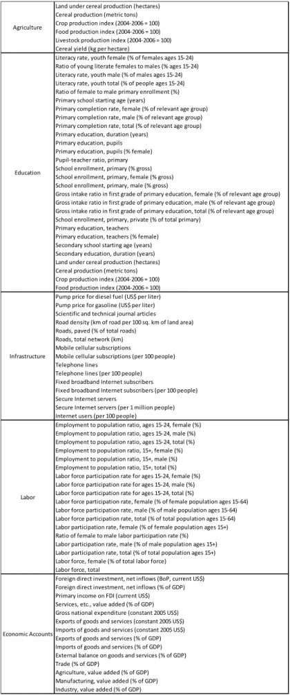
It is reasonable to consider only those variables that, although they are not reflected directly in the SAM or have the same format, are closely related to its structure and indirectly record the same socio-economic interactions of a certain country. Particularly, we have taken into account 77 variables covering the following fields:

 Agriculture: variables included here are intended to reflect the structure of the primary sector of each country and are related to the first 13 sectors of the harmonized SAM, including monoculture forestry and livestock.

 Education: this group of variables summarize, not only the level of education and literacy of the economies but also, along with labor, the linkages between education and the labor market as well as the degree of qualification of workers.

 Infrastructure: variables related to some industrial and service sectors of the SAM, such as transportation, communications or construction, among others.

 Labour: this set of variables shows the labor market conditions, which are latent in the accounts of retribution to workers in the structure of a SAM (value added), separated by skill level.

 Economic accounts: this group of variables is the one most clearly reflected in the activities and inter-sectorial linkages of a SAM and in the accounts relating to institutions, such as households, government or rest of the world.

From this exercise, 77 variables of WDI dataset have been retained.

Obtaining the proximity matrices between the initial 8 countries, generated by both SDGEII (28 variables) and by WDI (77 variables)

 First, taking directly the variables, standardized by case, corresponding to the 28 sectors of the SAM.

 Second, a factor analysis5 has been carried out, taking the resulting 7 factors for the subsequent analysis of similarity together with WDI database.

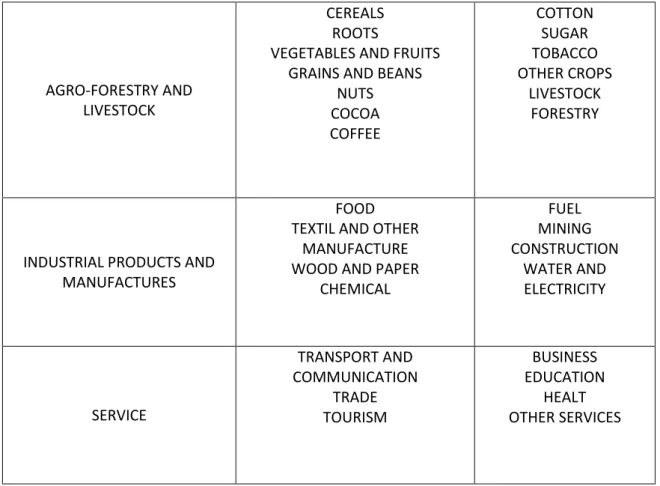
 Finally, we have created the following sub-sectors from the initial 28 variables: agriculture, monocultures, agro-forestry and livestock, industry-manufactures, services1 and services2 (education, health, and other services). Then, we have applied a factor analysis for each sub-sector, taking the resulting factors for the similarity analysis.

Considering these alternatives, we avoid the possibility of over-identification problem due to a large number of variables for a few countries. Also, grouping the initial 28 variables into sub-sectors allow us to control for differences that may arise in the processes of aggregation and disaggregation due to the lack of homogeneity in the initial data of the Social Accounting Matrices.

In the case of the selected variables from WDI dataset, we have considered the following possibilities:

• To conduct a factor analysis for WDI set of 77 variables and take the resulting factors for similarity analysis.

5

Factor analysis is “a procedure that postulates that the correlations or covariance between a set of observed variables, x’=[x1, x2,..., xq] arise from the relationship of these variables to a small number of underlying, unobservable, latent variables, usually known as the common factors” (Everitt 2002, p. 140). Our factor analysis is exploratory as we set no a priori constraints on the data structure. Factor analysis enables parsimonious reduction of the number of variables without losing the underlying pattern in the variation of variables (Hair et al. 1998). We use Kaiser’s criterion to determine the number of factors to be extracted. Accordingly, a factor is disregarded unless it can explain the variance of at least a single variable (“Eigenvalue” >1). To achieve explanatory power, we require our factors to explain at least 50% of the total cumulative variance in the data. We apply oblique rotation. This decision use to be more coherent within social-economic studies where totally uncorrelated variables are not frequent.

• To take into account the classification of WDI data set following the fields mentioned above. Then, we have applied a factor analysis for each subsector, taking the resulting factors for similarity analysis. Additionally, we have also considered the first factors of each subset.

• In addition, we have performed a cluster analysis for the initial 8 countries, considering SDGEII factors as the variables that determine the “club” membership. Then, we have implemented an analysis of variance (ANOVA) in order to observe which variables of WDI (and also factors and subset factors) better explain the classification of countries obtained in the cluster analysis.

From these variables/factors, and their possible combinations, we generate different proximity matrices for the 8 countries for which there is available SAM.

Correlation analysis of proximity matrices SDGEII-WDI and assignment of SAMs In order to obtain the “best” set of variables it is necessary to determine a criterion of similarity. Our proposal is to compare all combinations of proximity matrices SDGEII-WDI discussed above and calculate the correlation coefficient for each pair. The proximity matrix SDGEII-WDI with higher coefficient of correlation will indicate which set of variables/factors WDI is more similar to SDGEII and, therefore, it will allow us to assign to a country with lack of information the SAM of the most similar country among the 8 available.

Some of the 42 SSC have no data for any of the variables from the World Development indicators, falling out in the factor analysis. As a result, the group is reduced to 31 countries, the initial 8 and the 23 to which is assigned a particular SAM.

4. FIRST RESULTS AND DISCUSSION

In this study we have used two different sources of data:

I. Social accounting matrices of eight sub-Saharan countries, provided by the International Food Policy Research Institute (IFPRI). The available SAMs for each country and year are the following: Ghana (2005), Kenya (2003), Malawi (2007), Nigeria (2006), Mozambique (1998), Tanzania (1998), Uganda (2007) and Zambia (2001) (see references). These original SAMs present different levels of aggregation and, therefore, different number of sectors. Table 1 (Appendix 1) shows the sectors included in the original SAM of each country.

II. World Development Indicators Dataset (WDI) for the period 2000-2010, including variables belonging to the following categories: agriculture, education, labour and social protection, infrastructure and economic accounts (see appendix IV).

Shock of demand global economic impact index (SDGEII)

In this section, the outstanding characteristics of the production structure and the dynamics of the value chain in each country in terms of SDEGII are reported (appendix III). This vision of each individual economy as well as the comparison by subsectors allows us to better understand the reasons underlying the subsequent assignment of a given SAM in the multi-country analysis.

Graph 1 shows the values of SDGEII grouped by sub-sectors, so that it can be observed which countries get grouped or are closer in terms of production structure under different economic activities. Differences can be observed in both variability (dispersion in the graph) and dynamic potential (score in SDGEII) for each sector between countries.

In the primary sector (agriculture and monocultures), we can glimpse two more or less distinct groups, with Nigeria and Malawi showing the highest SDGEII scores. The same applies in the

case of agroforestry and livestock, where Tanzania and Zambia are left behind from the group. In the case of services (services 1), Ghana and, to a lesser extent, Mozambique, presents a lower lever effect.

Graph 1. SDGII by sub-sectors

Source: own calculations

Attending to the rest of sectors inside graph 1, in the case of the industry sector and services 2, very small dispersion is observed being all countries almost overlapped. However, there is a remarkable difference between both sectors in terms of activation of the economy. In this sense, the index suggests once again that service 2 (health, education,…) have great potential in the economic development of these SSC (they showed a high score in the SGDEII). It is not the same for the secondary sector.

Going further in details about each country, Ghana is characterized by a quite dynamic but undeveloped primary sector, except of Cereals and Cocoa. The same situation occurs in the case of Education and Health.

0 10 20 30 40 50 60 70 80 90 100 GHANA KENIA MALAWI NIGERIA MOZAMBIQUE TANZANIA UGANDA ZAMBIA

Kenya records high values in agriculture and natural resources, including some monocultures like Coffee and Sugar. It should be stressed the crucial lever effect of services, being Transport-Communication, Business and Education the main sectors.

Malawi shows great potential in agriculture, natural resources and services. However, this country only shows important presence for the primary sector, Business and, particularly, Trade and Health.

In the case of Mozambique, Roots, Nuts, Forestry and Livestock sectors stand out for SDGEII. The service sector has rather low values except Business. Considering the current size of the sectors, we must highlight the presence of Cereals, Crops, Business and Construction, in contrast to Health and Education, clearly an outstanding issue in this country.

Nigeria is strongly influenced by the production and exportation of the agro-food industry as well as oil extraction and exploitation of natural resources, affecting SDEGII values for all the related sectors.

In Tanzania, we can observe the positive lever effect of Cereals, Vegetables, Fruits, Livestock, Trade and Education. The latter along with Health, Trade, Tourism and Vegetables-Fruits play a crucial role in this economy.

Uganda is characterized by high values of SDGEII in sectors related to natural resources, Water-Electricity and monocultures, which lose significance when incorporating sectorial "size", in favor of Construction, Trade, Business and Education.

Zambia shows a hardly dynamic production structure with low inter-sectorial linkages, except for the potential impact of tourism, still underdeveloped.

SDGEII can be very useful to observe sectors with a great potential to boost the economy of a certain country, identifying which of them are able to strongly stimulate economic development through positive carry-over effects in other sectors during the production process (strong sectorial linkages, high SDGEII). However, it could happen that some of these sectors were not big enough to translate that potential into real effect on the productive structure of the country. In other words, sectors with high SDGEII but with low weight in terms of total VA.

Several possible reasons of this relative small size arise. Sometimes, this situation may come from the historical process of development and, then it could be reverted: these sectors should be seriously considered to be enhanced and perhaps prioritize. In this sense, SDGEII becomes a useful leading signal.

However it is possible that these sectors are "small" because they have to be "small". That is, there are certain limitations for which these sectors cannot grow or would be harmful to do so. These potential limitations may include lack or deterioration of natural resources and other environmental problems, geographic limitations (landlocked countries), geo-climatic or geophysical characteristics (soil conditions), property rights or land grabbing and food security among others.

In order to avoid these limitations, we point out, for further research, the use of a SDGEII weighted by the contribution of each sector to the total economy in terms of value added. Unfortunately, by using this second option, , we could be condemning countries to maintain in the future the same current production structure and, therefore, to a stagnation in the development process. Thus, it would be desirable a detailed analysis of the limiting factors for each sector and country.

Assignment of a Social Accounting Matrix to SSC with lack of information

As detailed in the methodology section, our first goal was to determine the better way to express the relationships between the SDGEII and the WDI indicators in order to reveal the highest correlation between them. With this aim, we computed the common Pearson coefficient among different transformations of our indicators obtaining the following results (table 1).

Table 1. Correlation of SDGEII and WDI variables by data transformation SDGEI \ WDI Factors using all of

the set

Factors by economic groups

Standardized 0.55** 0.43**

Factors

(for the total set)

0.41** _0.37

Factors

(by sub-sectors)

0.27 0.23

** 5% significance or more

Table 1 shows the results for all relevant combinations, discarding those that recorded very low coefficients. The highest correlation is obtained when considering the factors generated from the 77 WDI variables. This holds for both the 28 SDGEII standardized variables and for the factors obtained from these variables or to those obtained from the sub-sectors. In addition, these correlations are statistically significant at 5 percent in the first two cases. Hence, considering that this option is the one that better "reproduce" the behaviour of the SDGEII index, we will use it to assign SAMs to those countries with lack of information. It is worth noting that the correlation computed arise a significant value of 55% using this wide set of variables and assuring in some extent the good results that we can obtain when calculating the proximity measures that serve for our final goal: to associate each country without SAM with another one with SAM.

At this point, we already have common statistical information to all SSC and, therefore, we can assign a Social Accounting Matrix of the 8 countries with SAM to those who do not have. Following the mentioned criteria of similarity, the following table shows the resulting assignment.

Table 2. Sam Assignment Countries

with SAM GHANA KENIA MOZAMBIQUE TANZANIA UGANDA ZAMBIA

Countries without SAM Botswana (15.97) Congo, D. Rep. (3.95) Congo (7.42) Ivory Coast (4.46) Gambia (3.25) Lesotho (11.14) Mali (7.22) Mauritania (8.42) Senegal (3.01) Cameroon (2.11) Gabon (19.06) Sudan (3.97) Angola (10.3) Benin (2.69) Burkina Faso (7) Central Africa Rep. (2.83) Ethiopia (4.9) Guinea (5.8) Niger (8.39) Burundi (3.55) Madagascar (4.27) Rwanda (2.75) Swaziland (23.27) Average Within 7.0525 8.38 5.98 3.55 3.51 23.37 Variance Coefficient 0.600 0.905 0.435 0 0.216 0

In brackets, square Euclidean distance between pair of countries. Maximum 50.2 and minimum 0 (see table 5 in the appendix). Variance coefficient computed as standard deviation over average.

Source: own calculations

We can observe that Malawi and Nigeria are the most "different" countries, so that no other country is assimilated to them. By contrast, the socio-economic structures of Ghana and Mozambique in terms of SDGEII seem to be quite representative of what is happening in other economies in SSC, with 9 and 7 countries associates, respectively. The other countries are distributed fairly evenly between Kenya (3) Tanzania (1) Uganda (2) and Zambia (1).

In an attempt to summarise the “robustness” of each group of countries with an indicator, we can compute the average of the distances within each one. To measure the internal disparity of them, we can compute the standard deviation. By doing this, the group leading by

Mozambique could be considered the most homogenous (average 5.98 and standard deviation 0.435), joining 8 countries. It is worth noting that we would obtain very similar results for the group lead by Ghana just suppressing Botswana or Lesotho, clearly distorting these measures with distances over 10 points but joining a relative large number of countries too (10).

From these results, our hypothesis of “different groups inside SSC” can be totally confirmed. Clearly, several subsets of countries are derived from our analysis and, then, considering them as a whole when using different tools to simulate effects of FTA will produce confusing results.

5.

COMPARING THE RESULTS OF EXTERNAL TRADE LIBERALIZATION FOR

SUB SAHARA COUNTRIES USING AN ARCHETYPE AGAINST A GROUPS OF

ANALOGOUS COUNTRIES

The goal of this subsection is to illustrate the substantial differences in potential trade liberalization results when using some kind of SSC supposed archetype instead using several different SAMs taking the “nearest neighbour” in terms of economic structure similarity. In this sense, we have carried out three simulations to compute these differences: (i) 50% reduction of import tariffs, (ii) 10% increase in exports, and (iii) both effects at the same time.

For this exercise, 4 countries have been taken into account: Kenya, Nigeria, Uganda and Zambia, representing a total of 10 SSC following our previous results (Group A: Kenia, Cameroon, Gabon and Sudan. Group B: Nigeria. Group C: Uganda, Madagascar and Rwanda. Group D: Zambia and Swaziland). Alternatively, an average SAM of these countries has been computed.

As we have previously mentioned, this strategy pursues to illustrate the advantages of assigning the SAM of the most similar country in cases of lack of information instead an average country (unique SSC structure assumption). In these simulations, we have used the

CGE model proposed by the Partnership for Economic Policy (PEP) developed by Decaluwé et al (2013), conveniently arranged for the five SAM structures that we are using.

In the following tables, we show some of the results derived from our simulation. Although the analysis of the exact results in this simulation is not the main purpose of this exercise, a thick trace of these examples with some variables of interest serves to show the huge differences using an aggregate or using specific groups of countries. We will concentrate our comments in three groups of variables: measures of household income and consumption, public finances indicators, and three macro variables in relation to the aggregate economy.

Table 3. 50% import tariff reduction Simulation results in variation rates

VARIABLE Archetype Group A Group B Group C Group D Range (4 countries)

Total income of type h households

Rural -1.39 -1.05 -1.41 -3.31 -0.78 2.53 Urban -1.46 -1.02 -1.50 -3.35 -0.86 2.48 Real consumption budget

Rural 0.75 1.36 0.68 1.36 1.64 0.95 Urban 0.68 1.38 0.59 1.32 1.55 0.96 Total government income -3.07 -8.46 -2.08 -18.36 -14.68 16.28 Government savings -9.74 -72.89 -6.18 -65.42 73.92 146.82 Government final consumption of public

services 1.64 2.45 1.39 4.72 2.14 3.33 Real GDP at market prices 0.34 -0.39 0.54 -1.04 -0.91 1.58 Real gross fixed capital formation -14.90 -12.93 -15.01 -14.74 -9.18 5.82 Total investment expenditures -16.07 -14.94 -15.81 -18.82 -12.20 6.63

Source: own calculations

Coherently with the basic economic theory represented by the PEP 1-1 model, in this hypothetical and unilateral import tariff reduction, a decrease of government income and savings as well as a fall in investment and GDP is observed. Government expenditure in public services (that mainly records education and health in our example) records however positive effects. Regarding to household welfare, although both rural and urban register a negative

effect in terms of total income, it turns into positive impact when considering real consumption.

It is worth noticing the significant discrepancies in these results among groups and, consequently, the crucial errors can be committed when using the “Archetype” instead the most similar country strategy. In this sense, the second set of variables, particularly “Government savings” and “Total government income” exhibit the higher ranges of differences (146.82 and 16.28, respectively). For instance, when introducing a 50% cut on import tariffs rates, government savings would decline by 72.89 per cent for group A against a 73.92 per cent of increase in the case of Group D. On the other hand, the archetype records a fall of 9.74 per cent. In the case of the variation of the GDP, the archetype registers even different sign that A, B and D groups, obviously influenced by Nigeria. The same, although without change of sign, occurs for the other variables in this third group, as well as those representing the household income and consumption.

As shown in table 3, given this unilateral trade liberalization, urban households suffer a greater drop in total income and a smaller increase in real consumption than rural households. This better performance of rural households is true for the archetype and the other countries except group A. Therefore, if we take archetype as a reference to observe the effects of a reduction on import tariffs for Cameroon, Gabon and Sudan (countries that present more similarities to Kenya) we would be again committing significant errors regarding the impacts on different types of households.

Table 4. 10% world export price increase Simulation results in variation rates

VARIABLE Archetype Group A Group B Group C Group D Range (4 countries)

Total income of type h households

Rural 10.35 11.32 9.84 9.71 9.21 2.11 Urban 10.30 11.38 9.69 9.63 9.41 1.97

VARIABLE Archetype Group A Group B Group C Group D Range (4 countries)

Real consumption budget of type h households

Rural 2.52 3.50 2.36 2.28 3.11 1.22 Urban 2.47 3.55 2.22 2.20 3.30 1.35 Total government income 11.14 9.09 11.25 7.57 8.19 3.69 Government savings 35.38 70.45 33.87 26.46 -29.98 100.43 Government final consumption of public services -7.20 -6.94 -6.74 -7.01 -6.25 0.75 Real GDP at market prices 2.94 3.16 2.93 2.22 3.19 0.96 Real gross fixed capital formation 67.79 8.12 80.67 6.04 2.33 78.34 Total investment expenditures 67.79 15.78 90.43 11.59 6.44 83.99

Source: own calculations

Moving to the second simulation, the effects of an increase on the exports leads to a better performance of all the variables but “government final consumption of public services”, that records negative variations for all the economies. Once again, “government savings” presents the higher range (100.43), together with “total investment expenditures” (83.99) and “real gross fixed capital formation” (78.34). This means that these are the variables in which the errors will be more relevant if we take the archetype instead the most similar country. Particularly, in the case of group D government savings, the effect would be, not only lower but negative, driving to serious errors for a hypothetical economic policy.

Finally, going to a more realistic scenario where bilateral trade liberalization is performed, obviously negative and positive effects of the previous simulation schemas can be partially offset.

As in the other cases, public accounts estimations are the more affected by the simulation strategy selected. The government income and savings could change in a proportion that moves in a range to -43.14 to +48.74 points, depending of the group of countries observed and, the archetype solution produces a median solution totally erroneous for all the pseudo-represented countries (+24.16). In terms of investment, countries within group B show a totally different performance than the rest of the groups considered in this simulation,

recording an important positive increase in this indicator. Once again, considering all the countries as a whole would produce clearly biased results. The same idea applies for the differences observed in variables related with household agents, both rural and urban. There, four points of difference in the total range of results could be interpreted as a minor concern but it is worth noticing the huge impact of these changes in some variables that can be represent more than 75% of GDP. Additionally, these variables are intrinsically related with the main purpose of liberalization policies, in the sense that we are speaking about poorness and, in some way, in economic measures to reduce it.

Table 5. Both shocks: 10% increase in exports and 50% decrease in import tariffs Simulation results in variation rates

VARIABLE Archetype Group A Group B Group C Group D Range (4 countries)

Total income households

Rural 8.76 10.08 8.25 6.04 8.44 4.04 Urban 8.62 10.16 7.99 5.94 8.56 4.23 Real consumption budget of households

Rural 3.33 4.84 3.12 3.58 4.77 1.72 Urban 3.20 4.92 2.87 3.48 4.89 2.05 Total government income 7.61 0.02 8.84 -11.96 -7.38 20.80 Government savings 24.16 -7.71 26.66 -43.14 48.74 91.88 Government final consumption of public services -5.62 -4.68 -5.39 -2.67 -4.36 2.72 Real GDP at market prices 3.31 7.91 3.53 1.15 2.30 6.76 Real gross fixed capital formation 43.43 -4.66 64.90 -8.71 -7.11 73.61 Total investment expenditures 49.29 -0.25 72.14 -8.51 -6.54 80.64

Source: own calculations

Therefore, the main conclusion of this simulation is as follows. As we have mentioned before, there is no socioeconomic information (SAMs) available for certain countries in sub-Saharan Africa. In order to face with this problem of lack of information it is possible to consider the region as a whole, assuming high homogeneity between countries when performing different studies, particularly macroeconomic simulations. However, this study concludes that the errors committed (vs. a hypothetical SAM available for a country with a lack of information) are

significantly lower if we consider the SAM of the most similar country instead the archetype (Unique Sub-Saharan Africa). The simulation results of using a more disaggregated available structure between SSC are dramatically different and the policy conclusions derived from them could be totally different too when planning economic triggers to reduce poverty in African countries.

6.

CONCLUSIONS AND FINAL REMARKS

The main achievement of this study has been to propose a classification of the SSC in order to partially solve the problem of lack of statistical information in these countries and, then, do possible the analysis of the impact and effects of different macroeconomic policies, particularly, trade liberalization and FTA using the more affordable SAM structures for each country coming from the most similar country in the area. In order to bring this about, we have performed an analysis of similarity studying the correlations between proximity matrices generated by two databases: WDI, containing socioeconomic information for all countries and SDGEII, created index that records the dynamism of the production structure for the 8 SSC with available SAM. These are the main conclusion of the analysis:

First, it has been possible to assign a particular SAM to 23 countries with lack of information.

Second, Ghana and Mozambique appear to properly represent the potential and dynamism of the economy of sub-Saharan Africa. The SAMs of these countries is assigned to 18 countries. By contrast, none of the 23 countries is assimilated to the economies of Malawi and Nigeria.

Third, the highest correlation coefficient between proximity matrices WDI-SDGEII appears when taking into account the 7 factors resulting from factor analysis on the initial 77 variables of the WDI data set. This correlation is fairly stable when considering the initial 28 SDGEII

variables standardized by case, their factors and the factors aggregating by sub-sectors, showing the highest values for the 3 cases.

Finally, from the SDGEII values for the 8 countries we can draw some considerations (see appendix III). As expected, the primary sector and exploitation of natural resources is still the basis of the economies of this region of the world, while education stands out, ahead of health, as the most important lever of development for most countries. Also, it is one of the biggest challenges, as their weight in the total economy is still very small. By contrast, manufacturing and industry sectors show little potential for activation of the economy (Chart 1). Additionally, the dependence on monocultures is decisive in several countries, while Nigeria stands as the most differentiated economy due to the strong effect of oil extraction and agro-food industry.

Moving to the results of the trade liberalization estimate using the common strategy (considering SSC as a whole) against the groups of several countries as the more affordable strategy, we have showed how the same classical shocks (reduction of tariffs and increase in exports) can derive in very different consequences attending to the different economic structures within SSC. Unfortunately, to conduct specific simulation for each country is not possible due to the lack of statistical information. However, using any kind of global archetype for all the SSC is clearly a bad solution. The “median solution” produce by this kind of archetypes hides very different consequences for each country and, sometimes, even positive and negative not real compensations between countries. Knowing that our proposal of using groups of countries is not perfect, it could reduce the excessive common generalization in designing policies to reduce poverty as trade liberalization.

BIBLIOGRAPHY

Bénassy-Quéré, A. and Coupet, M., 2005. On the Adequacy of Monetary Arrangements in Sub-Saharan Africa. The World Economy 28 (3): 349–373.

Bourguignon, F., de Melo, J. and Suwa, A., 1991. Distributional Effects of Adjustment Policies: Simulations for Archetype Economies in Africa and Latin America. World Bank Economic

Review 5 (2): 339-366.

Condon N, Stern M (2010) The effectiveness of African Growth and Opportunity Act (AGOA) in increasing trade from Least Developed Countries: a systematic review. London: EPPI-Centre, Social Science Research Unit, Institute of Education, University of London. Available at: http://r4d.dfid.gov.uk/PDF/Outputs/SystematicReviews/AGOA-Report.pdf

De Arce, R. and Mahia, R. 2013. "An Estimation of the Economic Impact of Migrant Access on GDP: the case of the Madrid Region". International Migration, 51 (1), 169–185.

De Arce, R., Mahia, R., Medina, E. and Escribano, G. 2012. A Simulation of the Economic Impact of Renewable Energy Development in Morocco. Energy Policy, 46.335-345.

Decaluwé, B., Lemelin, A., Robichaud, V. and Maisonnave, H. (2013): PEP-1-1 (Single-Country, Static Version 2.1). Partnership for Economic Policy PEP, July 2013. Université Laval, Québec (Canada).

Diaz-Bonilla, E. and Reca, L. 2000. Trade and Agro Industrialization in Developing Countries: Trends and Policy Impacts. Agricultural Economics, 23, 3, 219–29.

Durlauf, S.N., Johnson, P., 1995. Multiple regimes and cross-country growth behavior. Journal

of Applied Econometrics 10, 365– 384.

Elamin, N and Khaira, H. 2004. Tariff Escalation in Agricultural Commodity Markets, in Food and Agriculture Organization of the United Nations (FAO), Commodity Market Review 2003– 2004, Rome: FAO.

Everitt, B.S., 2002. The Cambridge Dictionary of Statistics. 2nd Edition, Cambridge: Cambridge University Press.

Hair, F.J., Anderson, R.E., Tatham, R.L. and Black, W.C. (1998) Multivariate Data Analysis. 5th Edition, New Jersey: Prentice Hall.

Janvry, A. and Sadoulet, E., 2010. World Poverty and the Role of Agricultural Technology: Direct and Indirect Effects. The Journal of Development Studies, 38 (4): 1-26.

Johnson, S., Ostry, J. and Subramanian, A., 2008. Prospects for Sustained Growth in Africa: Benchmarking the Constraints. IMF Staff Papers, 2010, 57, 1, 119.

Kose, M. and Raymond Riezman, R., 2001. Trade shocks and macroeconomic fluctuations in Africa. Journal of Development Economics, 65 (1). 55-80.

Mohan, S., Khorana, S. and Choudhury, H. (2013), Why Developing Countries Have Failed to Increase Their Exports of Agricultural Processed Products. Economic Affairs, 33: 48–64.

Paap, R., Franses, P., van Dijk, D., 2005. Does Africa grow slower than Asia, Latin America and the Middle East? Evidence from a new data-based classification method. Journal of

Rae, A. and T. Josling (2003) ‘Processed Food Trade and Developing Countries: Protection and Trade Liberalization’, Food Policy, 28(2), 146–66.

Tadesse, B. and Fayissa, B. (2008), The impact of African growth and opportunity act (Agoa) on U.S. imports from Sub-Saharan Africa (SSA). Journal of International Development 20: 920–941. Data

Douillet, Mathilde; Pauw, Karl; Thurlow, James, 2012-07-25, “Replication data for: A 2007 Social Accounting Matrix for Malawi”, http://hdl.handle.net/1902.1/18578 International Food Policy Research Institute [Distributor] V1 [Version]

Thurlow, James, 2012, “Replication data for: A 2007 Social Accounting Matrix for

Uganda”,http://hdl.handle.net/1902.1/18662 International Food Policy Research Institute [Distributor] V1 [Version]

Nwafor, M., X. Diao, and V. Alpuerto. 2010. A 2006 Social Accounting Matrix (SAM) for Nigeria: Methodology and Results. Washington, D. C.: International Food Policy Research Institute (IFPRI) (datasets). http://www.ifpri.org/dataset/2006-social-accounting-matrix-nigeria-metho…

Breisinger, Clemens; James Thurlow; Duncan, Magnus. 2007. A 2005 Social Accounting Matrix (SAM) for Ghana. Ghana; Washington, D.C.: Ghana Statistical Services (GSS); International Food Policy Research Institute (IFPRI)(datasets). http://www.ifpri.org/dataset/ghana

Kiringai, Jane; Thurlow, James; Wanjala, Bernadette. 2006. A 2003 Social Accounting Matrix for Kenya. Nairobi; Washington, D.C.: Kenya Institute for Public Policy Research and Analysis (KIPPRA); International Food Policy Research Institute

(IFPRI)(datasets). http://www.ifpri.org/dataset/kenya-social-accounting-matrix-sam-2003 Zambia: Social Accounting Matrix, 2001. 2005. Washington, D.C.: International Food Policy Research Institute (IFPRI) (datasets). http://www.ifpri.org/dataset/zambia-0

Mozambique: http://www.ifpri.org/dataset/mozambique (1998) Tanzania: http://www.ifpri.org/dataset/tanzania-0 (1998)

APPENDIX

Table A.1 Harmonization of SAMs with 28 sectors

HARMOGENIZED SAM ACTIVITIES NIGERIA GHANA KENIA MALAWI MOZAMBIQUE TANZANIA UGANDA ZAMBIA

Rice x x x x x x Wheat x x x x x Maize x x x x x x x Barley x Sorghum x x x Millet x Other cereals x x x x x x Cassava x x x x x Yams x x Cocoyams x x Roots x x x Irish potato x Sweet potato x Fruits x x x horticulture x x x x

Banana and plantain x x

Matoke x Vegetables x x x x Cut flowers x Beniseed x Soyabeans x x Beans x x x x x Cowpea x

Pulses & oil seeds x x

Nuts x Groundnuts x x x Cashew x x x x COCOA Cocoa x x COFFEA Coffee x x x x COTTON Cotton x x x x x x x

SUGAR Sugar and sugar cane x x x x x x

TOBACCO Tobacco x x x x x x Other crops x x x x x x Rubber x x Sisal x Tea x x Oil palm x x x Cattle x x

Live goats and sheep x x x x

Live poultry x x

Other livestock x x x x x x

FORESTRY Forestry x x x x x x x x

Fish and fish meat x x x x x x x x

Beef x x x

Goat and sheep meat x x x x

Poultry meat x x x

Eggs x x

Milk and dairy products x x x

Other livestock meat x x x x

Beverages x x x x x x x

Processed food products x x x x x x x

Textiles and leather products x x x x x x x x Other manufactured products x x x x x x x

WOOD-PAPER Wood, wood products, furniture x x x x x x x x

Fertilizer x x x x

Other Chemicals x x x x x x x

Crude petroleum and natural gas x x x x x

Refined oil x x x x

Other mining x

mining x x x x x

Metal products x x x x

CONSTRUCTION construction x x x x x x x

WATER¬ELEC Electricity and water x x x x x x x

Road transport x

Transportation and other equipment x x x x Telecommunications, Post, broadcasting x x x x

Other transportation x

Transport services x x x x x x x

Trade x x x x x x

Wholesale and retail trade x

Hotel and restaurants x x x x x

Tourism x x

Financial institutions, Insurance, Business services x x x x x x x x

Real estate x x x x x x x

EDUCATION Education x x x x x x

HEALTH Health x x x x x x

Public administration x x x x x x x

public-non market services x

Private non profit organisations, Other services x x

other services x x x x x OTHER SS TRANS-COMM TRADE TOURISM BUSINESS TEXT-otherMANUFACTURES CHEM FUEL MINE CROPS LIVESTOCK FOOD CEREALS ROOTS VEGG&FRUIT GRAIN&BEANS NUTS

Table A.2

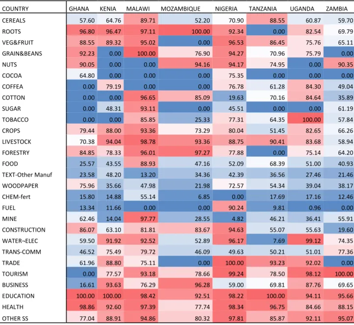
SDGEII by country

COUNTRY GHANA KENIA MALAWI MOZAMBIQUE NIGERIA TANZANIA UGANDA ZAMBIA CEREALS 57.60 64.76 89.71 52.20 70.90 88.55 60.87 59.70 ROOTS 96.80 96.47 97.11 100.00 92.34 0.00 82.54 69.79 VEG&FRUIT 88.55 89.32 95.02 0.00 96.53 86.45 75.76 65.11 GRAIN&BEANS 92.23 0.00 100.00 76.90 94.27 70.96 75.79 0.00 NUTS 90.05 0.00 0.00 94.16 94.17 74.95 0.00 90.35 COCOA 64.80 0.00 0.00 0.00 75.35 0.00 0.00 0.00 COFFEA 0.00 79.19 0.00 0.00 76.78 61.28 84.30 49.04 COTTON 0.00 0.00 96.65 85.09 19.63 70.16 84.64 35.89 SUGAR 0.00 48.31 93.11 0.00 45.51 0.00 0.00 61.19 TOBACCO 0.00 0.00 85.85 25.33 77.31 64.35 100.00 57.84 CROPS 79.44 88.00 93.36 73.29 80.04 51.45 82.65 66.26 LIVESTOCK 70.38 94.04 98.78 93.36 88.75 90.41 83.68 58.94 FORESTRY 84.85 78.33 96.01 97.27 77.88 0.00 75.14 64.20 FOOD 25.57 43.55 88.93 47.16 52.09 68.39 51.00 40.93 TEXT-Other Manuf 23.58 48.20 13.20 34.36 42.39 36.56 27.46 21.46 WOODPAPER 75.96 35.66 47.98 21.98 72.57 54.34 39.04 38.17 CHEM-fert 15.80 14.88 55.14 6.85 0.00 17.69 17.16 12.46 FUEL 13.34 11.66 0.00 0.00 90.24 9.81 0.96 0.00 MINE 62.46 14.04 97.77 28.55 4.82 46.21 36.41 55.91 CONSTRUCTION 86.07 63.10 81.81 83.67 94.63 55.07 55.63 19.60 WATER¬ELEC 59.50 91.92 92.52 52.89 96.17 7.69 99.12 74.35 TRANS-COMM 46.52 75.49 79.72 46.09 49.63 50.21 51.01 77.36 TRADE 61.96 88.80 75.11 0.00 100.00 93.23 92.02 0.00 TOURISM 0.00 77.57 93.18 78.66 99.24 78.50 98.12 100.00 BUSINESS 16.61 93.63 76.29 96.28 59.00 69.81 87.76 69.65 EDUCATION 100.00 100.00 98.42 92.51 98.22 100.00 94.11 95.66 HEALTH 98.86 92.60 97.39 77.74 98.34 96.75 84.66 88.15 OTHER SS 77.04 88.91 94.86 80.32 97.81 85.87 92.11 95.07

Table A.3 Proximity Matrix

Country Ghana Kenya Malawi Mozambique Nigeria

Tanzania, United Republic of Uganda Zambia Angola 10.82 19.65 14.76 10.30 12.07 22.80 19.09 11.78 Benin 7.74 11.51 14.08 2.69 11.75 10.29 8.07 13.04 Botswana 15.97 21.89 37.58 43.86 32.96 37.71 34.75 18.68 Burkina Faso 15.73 24.42 26.86 7.00 20.54 10.22 21.65 20.74 Burundi 12.35 10.65 8.15 8.04 16.80 3.55 6.17 15.33 Cameroon 8.22 2.11 9.29 9.16 9.85 8.15 4.93 7.82

Central African Republic 16.04 15.57 14.89 2.83 16.29 9.56 16.46 19.96

Congo, Dem. Rep. 3.95 21.04 22.62 13.23 15.80 19.87 16.03 23.57

Congo 7.42 19.56 21.70 17.45 14.84 21.57 19.86 7.75 Ivory Coast 4.46 9.65 17.64 8.92 9.34 12.73 15.30 7.58 Ethiopia 16.01 19.48 16.22 4.90 14.80 6.42 15.95 17.48 Gabon 20.93 19.06 39.68 44.74 30.96 43.29 27.95 24.20 Gambia, The 3.25 11.64 21.22 14.08 16.67 11.87 13.58 9.93 Guinea 6.27 14.61 18.66 5.80 10.75 10.35 11.28 8.79 Lesotho 11.14 17.01 15.58 21.16 24.94 24.38 32.87 15.43 Madagascar 9.31 11.54 4.78 9.43 15.88 5.49 4.27 9.10 Mali 7.22 15.85 21.48 9.46 9.88 18.28 21.36 11.04 Mauritania 8.42 15.57 22.22 21.05 15.27 26.96 25.49 11.01 Niger 16.91 24.03 24.75 8.39 15.54 14.78 29.73 16.41 Rwanda 16.47 14.18 7.47 13.12 21.41 6.78 2.75 15.42 Senegal 3.01 17.45 22.72 14.85 18.43 17.19 18.27 11.87 Sudan 12.19 3.97 19.22 11.89 5.00 10.16 14.13 9.51 Swaziland 30.61 24.23 40.12 39.75 37.25 46.88 50.28 23.37

Source: own calculations

The proximity matrix between the 8 countries with available SAM and the 23 that do not have is shown. Ghana records the lowest values (deeper blue) and therefore greater similarity to other countries in terms of production structure. The opposite occurs with Nigeria and Malawi (deeper red). Tanzania deserves special mention because, while showing very low values of distance, there is almost always another country with a lower value, so only one country is assigned (Burundi). Similarly, although each and every country with lack of information is assigned to a particular SAM (the one of the most similar country), the value of the distance to the chosen country varies considerably, as well as the dissimilarity compared to the other 7. Botswana, Gabon and Swaziland are presented as the most "different" or less similar to other countries, while Cameroon records relatively low values for virtually all 8 countries. Cameroon, Benin and Rwanda show the lowest assignment values, below 3 (high similarity), while Swaziland is assimilated to the SAM of Zambia with a value of 23.37.

Table A.4. World Development Indicators used

Land under cereal production (hectares) Cereal production (metric tons) Crop production index (2004-2006 = 100) Food production index (2004-2006 = 100) Livestock production index (2004-2006 = 100) Cereal yield (kg per hectare)

Literacy rate, youth female (% of females ages 15-24) Ratio of young literate females to males (% ages 15-24) Literacy rate, youth male (% of males ages 15-24) Literacy rate, youth total (% of people ages 15-24) Ratio of female to male primary enrollment (%) Primary school starting age (years)

Primary completion rate, female (% of relevant age group) Primary completion rate, male (% of relevant age group) Primary completion rate, total (% of relevant age group) Primary education, duration (years)

Primary education, pupils Primary education, pupils (% female) Pupil-teacher ratio, primary School enrollment, primary (% gross) School enrollment, primary, female (% gross) School enrollment, primary, male (% gross)

Gross intake ratio in first grade of primary education, female (% of relevant age group) Gross intake ratio in first grade of primary education, male (% of relevant age group) Gross intake ratio in first grade of primary education, total (% of relevant age group) School enrollment, primary, private (% of total primary)

Primary education, teachers Primary education, teachers (% female) Secondary school starting age (years) Secondary education, duration (years) Land under cereal production (hectares) Cereal production (metric tons) Crop production index (2004-2006 = 100) Food production index (2004-2006 = 100) Pump price for diesel fuel (US$ per liter) Pump price for gasoline (US$ per liter) Scientific and technical journal articles

Road density (km of road per 100 sq. km of land area) Roads, paved (% of total roads)

Roads, total network (km) Mobile cellular subscriptions

Mobile cellular subscriptions (per 100 people) Telephone lines

Telephone lines (per 100 people) Fixed broadband Internet subscribers

Fixed broadband Internet subscribers (per 100 people) Secure Internet servers

Secure Internet servers (per 1 million people) Internet users (per 100 people)

Employment to population ratio, ages 15-24, female (%) Employment to population ratio, ages 15-24, male (%) Employment to population ratio, ages 15-24, total (%) Employment to population ratio, 15+, female (%) Employment to population ratio, 15+, male (%) Employment to population ratio, 15+, total (%) Labor force participation rate for ages 15-24, female (%) Labor force participation rate for ages 15-24, male (%) Labor force participation rate for ages 15-24, total (%)

Labor force participation rate, female (% of female population ages 15-64) Labor force participation rate, male (% of male population ages 15-64) Labor force participation rate, total (% of total population ages 15-64) Labor participation rate, female (% of female population ages 15+) Ratio of female to male labor participation rate (%)

Labor participation rate, male (% of male population ages 15+) Labor participation rate, total (% of total population ages 15+) Labor force, female (% of total labor force)

Labor force, total

Foreign direct investment, net inflows (BoP, current US$) Foreign direct investment, net inflows (% of GDP) Primary income on FDI (current US$)

Services, etc., value added (% of GDP) Gross national expenditure (constant 2005 US$) Exports of goods and services (constant 2005 US$) Imports of goods and services (constant 2005 US$) Exports of goods and services (% of GDP) Imports of goods and services (% of GDP) External balance on goods and services (% of GDP) Trade (% of GDP)

Agriculture, value added (% of GDP) Manufacturing, value added (% of GDP) Industry, value added (% of GDP) Agriculture

Education

Infrastructure

Labor

Table A.5. SDGEII variables computed

AGRO-FORESTRY AND LIVESTOCK

CEREALS ROOTS

VEGETABLES AND FRUITS GRAINS AND BEANS

NUTS COCOA COFFEE COTTON SUGAR TOBACCO OTHER CROPS LIVESTOCK FORESTRY

INDUSTRIAL PRODUCTS AND MANUFACTURES

FOOD TEXTIL AND OTHER

MANUFACTURE WOOD AND PAPER

CHEMICAL FUEL MINING CONSTRUCTION WATER AND ELECTRICITY SERVICE TRANSPORT AND COMMUNICATION TRADE TOURISM BUSINESS EDUCATION HEALT OTHER SERVICES