Spectrum simulation of rough and nanostructured targets from their 2D and 3D image by Monte Carlo methods

  1  

Spectrum simulation of rough and nanostructured targets from their 2D and 3D

image by Monte Carlo methods

François Schiettekatte and Martin Chicoine Regroupement Québécois sur les Matériaux de Pointe (RQMP), Département de Physique, Université de Montréal, Montréal, QC, Canada

Abstract

Corteo is a program that implements Monte Carlo (MC) method to simulate ion beam analysis (IBA) spectra of several techniques by following the ions trajectory until a sufficiently large fraction of them reach the detector to generate a spectrum. Hence, it fully accounts for effects such as multiple scattering (MS). Here, a version of Corteo is presented where the target can be a 2D or 3D image. This image can be derived from micrographs where the different compounds are identified, therefore bringing extra information into the solution of an IBA spectrum, and potentially significantly constraining the solution. The image intrinsically includes many details such as the actual surface or interfacial roughness, or actual nanostructures shape and distribution. This can for example lead to the unambiguous identification of structures stoichiometry in a layer, or at least to better constraints on their composition. Because MC computes in details the trajectory of the ions, it simulates accurately many of its aspects such as ions coming back into the target after leaving it (re-entry), as well as going through a variety of nanostructures shapes and orientations. We show how, for example, as the ions angle of incidence becomes shallower than the inclination distribution of a rough surface, this process tends to make the effective roughness smaller in a comparable 1D simulation (i.e. narrower thickness distribution in a comparable slab simulation). Also, in ordered nanostructures, target re-entry can lead to replications of a peak in a spectrum. In addition, bitmap description of the target can be used to simulate depth profiles such as those resulting from ion implantation, diffusion, intermixing, etc. Other improvements to Corteo include the possibility to interpolate the cross-section in angle-energy tables, and the generation of energy-depth maps.

  2   1. Introduction

Currently, mainstream ion beam analysis (IBA) spectra simulation software is based on a description of samples in the form of layers or slabs, i.e. the sample is represented as a number of horizontal slabs with variable width and composition. Roughness is usually treated by carrying out several sub-simulations considering a layer thickness distribution, but even in that case, this imposes the approximation of treating all samples as laterally homogeneous. In many cases, the experimentalist also has access, for example, to cross-sectional transmission electron microscopy (TEM) images. Relying on that extra information about the sample description would impose a strong constraint on the solution. Indeed, it is often possible to obtain a perfect fit with slab simulations, but it does not mean that the solution found is the only possible one, and it can remain elusive to interpret, for example, a layer thickness distribution in terms of features observed in the sample. Hence, there is always the risk of over-interpreting an experimental spectrum, i.e. draw conclusions from data that the measurement does not actually allow. Conversely, the lack of appropriate tools to extract all the information available in a spectrum can lead to under-interpretation.

In this paper, we present the implementation in the IBA simulation program Corteo [1] of using a bitmap generated from a micrograph (TEM, scanning electron microscopy, atomic force microscopy (AFM), etc.) as the description of the sample. As an example, a TEM image can give information on the different phases present in a sample and how they are distributed, but there are often ambiguities about their composition. Rather than trying to reproduce an experimental spectrum by fitting, the user only has to test if an interpretation of the image complies with the experimental IBA spectrum by assigning compositions to the different parts of the image and running a simulation. This approach can actually be used with two- or three-dimensional bitmap representations of a sample. Incidentally, it can also be use to simulate the spectrum obtained from depth profiles, such as implantation or diffusion.

We use the Corteo code, which implements the Monte Carlo (MC) method of trajectory computation to simulate IBA spectra [1]. Early implementations of pixel sample representation already exist, namely MAST [2], or more recent ones [3]. They therefore take into account lateral inhomogeneity, which is a step further than considering homogeneous slabs, but their approach boils down to compute an equivalent thickness distribution. Trajectories featuring multiple scattering are not computed directly in the 3D structure. An implementation of 2D or 3D sample features in an MC simulation program has been presented for MCERD [4], in which it was shown that AFM images could be used as an input for surface roughness. NDF [5] can simulate abstract geometrical shapes such as quantum dots [6]. Also, SIMNRA [7] version 7 will introduce 2D bitmap sample description, but simulations will not take double scattering into account[8].

The strategy of using an image as a description for a sample is easy to implement in the framework of MC trajectory computation methods. First, ion trajectories are tracked in real space, so it is straightforward to know where ions are, i.e. in which pixel/material they are. This method also naturally samples many possible trajectories, including large-angle multiple scattering (MS) and actual detector geometry. The user has to provide an image representing the sample structure in the form of a bitmap or voxel map that uses a limited number of colors. Each color represents a particular material. A layer representing a flat substrate can also be included in

  3   the simulation. A rough substrate can be simulated by adding a rough layer that has the same composition as the substrate layer at the bottom of the bitmap.

Incidentally, description of targets as images offers the possibility to generate artificial profiles, which makes easier the simulation of depth profiles such as those resulting from ion implantation, diffusion, intermixing, etc. Users of Corteo version 2015 can generate bitmaps from arbitrary depth profile functions and obtain the corresponding simulated spectrum.

This paper also presents other improvements to Corteo: the possibility to interpolate the cross-section in angle-energy tables, and the generation of energy-depth maps.

2. Comparison with experimental results

Figure 1 shows an example of how the new version of Corteo can be used. Left is a TEM micrograph of a Ni-Si layer on a Si substrate [9]. There is a NiSi phase (as identified from a fast Fourier transform of the TEM image) and a phase identified by a question mark that could be either NiSi or NiSi2. The micrograph is transformed in a bitmap on the right with colors

associated with the different phases: blue and red for NiSi, purple for Si. The color black is reserved for vacuum. In Fig. 1(c), the dots represent the experimental data, measured with a 500 keV He beam. The green curve is a SIMNRA simulation considering a layer of 150×1015 Ni0.5Si0.5/cm2 with a thickness distribution of 70×1015 Ni0.5Si0.5/cm2 on a Si substrate. We get a

good fit with this thickness distribution but it is difficult to relate this information to the features in the TEM image. The solid red line is a Corteo simulation of the bitmap assuming that the green region is NiSi2 while the dotted red line assumes that it is NiSi. We see that the simulation that

assumes NiSi2 for the green region gives a much better agreement, so we can conclude that this

Figure 1. (a) Cross-section TEM micrograph of a NiSi/Si sample. (b) Corresponding bitmap. (c) Experimental data (blue dots), SIMNRA simulation (green line), Corteo simulation assuming that the green region is NiSi2 (solid red line) and assuming that the green region is NiSi (dotted red line).

(a) (b)

  4   region is indeed NiSi2. The agreement is not perfect, but the simulation is obtained without any

fitting parameter (except the incident charge). Rather than fitting, the procedure simply indicates if the composition assigned to the different regions complies or not with the measurement.

We then check if such detailed description of the sample is necessary since the resolution of such RBS analysis is typically of the order of a few nm. It may not be necessary in these conditions to have bitmaps that are overly detailed. Indeed, taking the example of Fig. 1, a simulation carried out with bitmap resolution of 0.5 pixel/nm show no significant difference from one carried out with a resolution of 14.6 pixels/nm. On the other hand, calculation time is not dramatically affected by bitmap resolution. In our tests, going from 14.6 pixel/nm with a 2048 pixels wide image to 0.5 pixel/nm with a 32 pixels wide image only decrease by a factor of 2 the computation time.

3. Test Cases 3.1 Rough layers

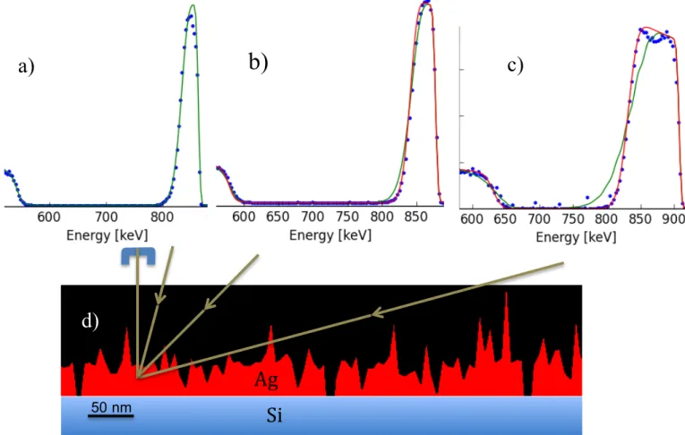
Corteo simulations with bitmap target description are also useful to test different effects on IBA such as target re-entry in rough layers. Figure 2 shows Corteo simulations (dots) of a hypothetical rough Ag layer on a flat Si substrate with a 1 MeV He beam. The bitmap representation of the sample is shown in Figure 2 (d). The thickness of the Ag layer is 153 × 1015

at./cm2, with a full width at half maximum (FWHM) thickness distribution of 117 × 1015 at./cm2.

Figure 2. Corteo (dots) and SIMNRA (solid lines) simulations of a (153±117) × 1015 at./cm2 Ag layer on a Si substrate for (a) 15°, (b) 45°, and (c) 75° incident angles. The bitmap representing the sample is shown in (d), with the lines representing the different angles of incidence.

c)

b)

Si

Ag

a)

d)

  5   (In this graph, we use SIMNRA as a tool to tell us how trajectory re-entry affects the apparent roughness, since thickness distribution is a fittable parameter. It is worth mentioning that SIMNRA version 6 is not intended to treat laterally inhomogeneous targets. This will be implemented in version 7.) The detector is placed along the sample surface normal. From Fig. 2 (a), where the incidence angle is close to normal (15°), we see that SIMNRA (green curve) and Corteo simulations with the same parameters (including the same thickness distribution) give very similar results, especially along the low-energy tail of the main peak. When increasing the angle of incidence to 45°, Fig. 2 (b), a departure starts to appear between the green curve, corresponding to a SIMNRA simulation with the same parameters as in (a), and Corteo. In order to reproduce the Corteo simulation, one has to consider a thickness distribution that is 2/3 of its actual value (red curve). The effect further extends at 75° incidence where the thickness distribution in a slab simulation has to be reduced to 44% of its actual value to reproduce the spectrum generated by Corteo. This example is meant to outline the effect of trajectory re-entering the target: it decreases the apparent thickness distribution in a slab simulation. Indeed, as the incidence angle increases, no ion can hit the target thinnest locations, neither can they maintain their trajectory only along the thickest parts. They rather cross several features of the target and it results in an apparent smoothing of the surface. Of course, the effect will depend on the aspect ratio of the roughness, not only on its vertical distribution. At a given incidence angle, sharp peaks may lead to re-entry effects, while layers with the same thickness distribution but consisting of much wider features will not be subject to the effect.

3.2 Gratings

Figure 3 shows Corteo simulations of an Ag grating on a Si substrate as a function of the beam incidence angle with respect to the sample surface normal. 2D images actually have periodical boundary conditions not only along lateral directions but also along depth, i.e. this structure is actually a grating and not 3D pillars. At normal beam incidence, the blue and green spectra features the expected two-step shape resulting from the fact that ions either cross a thick or thin section of the sample. The blue line at 0° shows the spectrum assuming straight-line trajectories (no MS) while the green line includes MS in the simulation. We see that the effect of MS is significant. The scattering yield is lower at low energy (below 600 keV) when we take MS into account. This is explained by the fact that events contributing counts below 600 keV involve

Figure 3. Corteo simulations of the Ag grating shown on the left side as a function of the incident angle. The blue line at 0° assumes straight-line trajectories (no MS).

  6   ions that followed a trajectory that never leaves a wall. When MS is included, there are non-negligible chances that they become deflected sufficiently to leave the wall, so they will never reach the detector with energies in this range.

As the angle increases, new peaks appear because of when the beam exits a wall, it may enter in the next one, producing multiple times the energy loss of a single wall, and causing a replication of the feature. At high incidence angle, the peaks become wider, the beam continuouly enters and leave the target, and the grating progressively appears like a uniform thick layer. 3.3 Three-dimensional targets

Figure 4 shows 3-dimensionnal structures and their simulated Corteo spectra. Corteo can read the .xraw format of 3D images generated using the MagicaVoxel program [10]. Simulations are carried out considering a He 500 keV beam. The first structure consists in a layer of Ag nanoparticles in a Si matrix on a Si substrate (a). On its corresponding spectrum at 7° incident angle and 3° detector angle (green line), we see that there is a dip in the Si signal (indicated by

(a) (b)

(c) (d)

Figure 4. Corteo simulations of 3D structures. (a) Ag nanoparticles in a Si matrix (cut-view) and (b) its corresponding spectra. (c) An Ag open nanostructure on a Si substrate and (d) its corresponding spectra. Blue lines are for 70° beam incident angle and for 60° detector position. Green lines are for 7° beam incident angle and 3° detector position. Angles with respect to the surface normal. Image in pannel (c) is an example of 3D picture provided with the voxel edition software MagicaVoxel [10].

  7   arrow) that corresponds to the Ag nanoparticles. But there is little to be learned from these spectra in terms of sample structure. The same applies for the second structure, which consists in an open Ag nanostructure. However, knowing shape of the structures from imaging techniques, one can simulate their spectrum to see if it complies with the measurement, and determine their composition.

4. Other improvements to Corteo 4.1 Cross-section interpolation

This new Corteo version implements the interpolation of tabulated cross-sections. Because of MS, the cross-sections must be known not only at the detector angle but at all possible angles, since trajectories can feature collisions at any angle. For example, Moser et al. [11] have computed such cross-section data tabulated as a function of angle and energy for the case of p-p. The new version of Corteo includes a script to generate such energy-angle tables for elastic non-Rutherford-backscattering cross-section from the data available from Alex Gurbich’s SigmaCalc website [12]. Nuclear reaction analysis (NRA) data will also be possible, provided that the cross section is provided at most angles.

4.2 Energy vs depth maps

Finally, Corteo now offers the possibility to generate Energy vs depth maps. This is a first step towards the implementation of PIXE simulations in Corteo, in order to include the effect of MS and actual target image in PIXE interpretation.

5. Conclusion

The main improvement of the new version of Corteo is its ability to use an image as the sample description. There will be at least two programs publicly available for pixel-based target IBA simulation: Corteo and SIMNRA. The main advantage of Corteo over SIMNRA is its ability to simulate MS events in such pixel-based targets. The intended use is to start from a real image of a sample (a cross-sectional TEM micrograph, for example), assign compositions to its different parts, and test if the resulting simulation agrees with the measured IBA spectrum. Still, it does not do miracles, e.g. structures with juxtaposed grains about same size and different materials will give the same solution if one grain is assigned to material A and the other to B or vice-versa. Complementary info is needed, e.g. identification of phases by electron diffraction or the presence or absence of some elements by, e.g., electron energy loss spectrometry, but once such ambiguity is removed, IBA will give the quantitative composition.

Other improvements to Corteo include the possibility to simulate the spectrum of arbitrary depth profiles, to interpolate the cross-section in angle-energy tables, and the generation of energy-depth maps. Corteo is free, open-source, and distributed along the terms of the General Public Licence [13].

  8   Reference

[1] F. Schiettekatte, Fast Monte Carlo for ion beam analysis simulations, Nucl. Instruments Methods Phys. Res. Sect. B Beam Interact. with Mater. Atoms. 266 (2008) 1880–1885. doi:10.1016/j.nimb.2007.11.075.

[2] Z. Hajnal, E. Szilágyi, F. Pászti, G. Battistig, Channeling-like effects due to the

macroscopic structure of porous silicon, Nucl. Instruments Methods Phys. Res. Sect. B Beam Interact. with Mater. Atoms. 118 (1996) 617–621.

doi:10.1016/0168-583X(96)00245-5.

[3] S.L. Molodtsov, A.F. Gurbich, C. Jeynes, Accurate ion beam analysis in the presence of surface roughness, J. Phys. D. Appl. Phys. 41 (2008) 205303.

doi:10.1088/0022-3727/41/20/205303.

[4] E. Edelmann, K. Arstila, J. Keinonen, Bayesian data analysis for ERDA measurements, in: Nucl. Instruments Methods Phys. Res. Sect. B Beam Interact. with Mater. Atoms, 2005: pp. 364–368. doi:10.1016/j.nimb.2004.10.071.

[5] N.P. Barradas, C. Jeynes, R.P. Webb, Simulated annealing analysis of Rutherford backscattering data, Appl. Phys. Lett. 71 (1997) 291. doi:10.1063/1.119524.

[6] N.P. Barradas, Can quantum dots be analysed with macrobeam RBS?, Nucl. Instruments Methods Phys. Res. Sect. B Beam Interact. with Mater. Atoms. 261 (2007) 435–438. doi:10.1016/j.nimb.2007.04.183.

[7] M. Mayer, SIMNRA, a simulation program for the analysis of NRA, RBS and ERDA, in: AIP Conf. Proc., 1999: pp. 541–544. doi:10.1063/1.59188.

[8] M. Mayer, Private communication.

[9] P. Turcotte-Tremblay, M. Guihard, S. Gaudet, M. Chicoine, C. Lavoie, P. Desjardins, et al., Thin film Ni-Si solid-state reactions: Phase formation sequence on amorphized Si, J. Vac. Sci. Technol. B. 31 (2013) 051213.

[10] MagicaVoxel, http://voxel.codeplex.com.

[11] M. Moser, P. Reichart, C. Greubel, G. Dollinger, Differential proton–proton scattering cross section for energies between 1.9MeV and 50MeV, Nucl. Instruments Methods Phys. Res. Sect. B Beam Interact. with Mater. Atoms. 269 (2011) 2217–2228.

doi:10.1016/j.nimb.2011.02.017.

[12] SigmaCalc, http://sigmacalc.iate.obninsk.ru/. [13] F. Schiettekatte, Corteo website,