Bias - variance tradeoff of soft decision trees
Cristina Olaru University of Li`ege Montefiore Institute B28 B4000, Li`ege, Belgium olaru@montefiore.ulg.ac.be Louis Wehenkel University of Li`ege Montefiore Institute B28 B4000, Li`ege, Belgium L.Wehenkel@ulg.ac.be AbstractThis paper focuses on the study of the error composition of a fuzzy deci-sion tree induction method recently proposed by the authors, called soft decision trees. This error may be ex-pressed as a sum of three types of error: residual error, bias and vari-ance. The paper studies empirically the tradeoff between bias and vari-ance in a soft decision tree method and compares it with the tradeoff of classical crisp regression and classifi-cation trees. The main conclusion is that the reduced prediction variance of fuzzy trees is the main reason for their improved performance with re-spect to crisp ones.
Keywords: Fuzzy Decision Tree, Classification, Bias, Variance
1 Introduction
Fuzzy decision tree induction is a combination between fuzzy reasoning and automatic learn-ing based on decision tree induction. It is a model concerned with the (automatic) design of fuzzy if-then rules in a tree structure. It is used in classification problems ([1, 7, 6, 12]) in most of the cases but sometimes also in re-gression problems ([10]).
The introduction of the fuzzy environment in the decision tree induction technique has been suggested within the fuzzy decision tree com-munity for three reasons: i) in order to enlarge the use of decision trees towards the ability to
manage fuzzy informationin the form of fuzzy inputs, fuzzy classes, and fuzzy rules manipu-lation, ii) in order to improve their predictive accuracy and respectively iii) in order to ob-tain reduced model complexity.
Building a fuzzy decision tree model is in most of the literature solely a question of tree growing. We speak about a top-down induction either as a crisp tree that after-wards is fuzzified, or as a tree that directly integrates fuzzy reasoning during the growing phase. The numerical inputs must be fuzzified (transformed from continuous values to fuzzy values) and this fuzzification step is rarely au-tomatic. There are approaches that consider also a pruning stage after growing in order to tradeoff better the model to data. A few au-thors have implemented after growing, also a global optimization phase of some parameters of the model. A global optimization aims at tuning the parameters of the model not any-more based on local learning samples but on the whole learning set and the already identi-fied structure of the tree.
We have proposed, explained and validated in reference [8] a complete fuzzy decision tree technique, called soft decision tree induction. The main objective of the present paper is to verify quantitatively the conjecture that the accuracy improvement of soft vs crisp trees is essentially a consequence of the reduced vari-ance of soft trees with respect to crisp ones. The paper is organized as follows. Sec-tion 2 explains intuitively the soft decision tree (SDT) method. Section 3 defines the bias-variance tradeoff in a SDT. Section 4 presents the experimental results concerning the bias-variance tradeoff in a SDT and
sec-tion 5 ends the paper with some conclusions.
2 Soft decision tree induction
A soft decision tree is a method able to par-tition the input space into a set of rectangles and then approximate the output in each rect-angle by a smooth curve, instead of a constant or a class like in the case of crisp tree-based methods. A soft tree is an approximation structure to compute the degree of member-ship of objects to a particular class (or con-cept) or to compute a numerical output of objects, as a function of the attribute values of these objects. The goal is to recursively split the input space into (overlapping) sub-regions of objects which have the same mem-bership degree to the target class (in the case of classification problems) or the same out-put value (in the case of regression problems). As in any tree-based approach, the hypothesis space of a soft decision tree model is a family of structures. A soft decision tree structure is determined by the graph of the tree and by the attributes attached to its test nodes. The parameters in all the test nodes together with the labels of all the terminal nodes repre-sent the parameters of the tree-based model. There is a search over both structure and pa-rameter spaces so as to learn a model from experience.
We now give an overview of our SDT method1
. The process starts by growing a “sufficiently large” tree using a set of objects called growing set GS. Tree nodes are succes-sively added in a top-down fashion, until stop-ping criteria are met. Then the grown tree is pruned in a bottom-up fashion to remove its irrelevant parts. At this stage, the hold-out technique is used which makes use of an another set of objects, called the pruning set P S. Next, a third step could be either a refit-tingstep or a backfitting step. Both consist of tuning certain parameters of the pruned tree model in order to improve its approximation capabilities further. These steps may use the whole learning set LS = GS ∪ P S or only the growing set GS. At the end of every inter-mediate stage, the obtained trees (fully de-veloped, pruned, refitted or backfitted) may
1
To save space we recall only the basics and ask the reader to kindly refer to [8] for details.
be tested. A third sample, independent from the learning set, called test set T S, is used to evaluate the predictive accuracy of these trees.
The growing procedure of a SDT follows the same principles as the crisp decision tree in-duction, only the partitioning procedure is different, being a fuzzy partitioning and not anymore a crisp partitioning. In our method, its objective is to determine in a node the best attribute a for splitting, the cutting point pa-rameter α, the degree of fuzziness β of the fuzzy partitioning and the labels of the two successors of the node. For this, an error function of squared error type adapted to the fuzzy framework is minimized. The strategy consists in decomposing the search into two parts: first, searching for the attribute a and threshold α at fixed null β, as if the node would be crisp; for this, strategies adapted to the fuzzy case from CART [2] regression trees are used; second, with the found attribute and threshold α kept frozen, searching for width β by Fibonacci search, and for every β value, updating labels in the successor nodes by lin-ear regression formulas.
Next, the pruning stage aims at finding a sub-tree of the large sub-tree obtained at the growing stage, which presents the best error computed on the pruning set. The strategy consists of three steps: firstly, all the test nodes of the full tree are sorted by increasing order of their relevance to the tree error, secondly, the nodes from the previous list are removed one by one in the established order and the result is a sequence of subtrees. And finally, the best subtree in terms of error is selected by the so-called “one-standard-error-rule”.
Then, the objective of the refitting step, given a tree and a refitting set of objects is to op-timize the labels in all the terminal nodes. It is a linear regression optimization problem, in practice fast and efficient in terms of accuracy. A more complex optimization stage is back-fitting whose objective, given a tree and a backfitting set, is to find not only the labels in terminal nodes but also the parameters α and β in all the test nodes, by minimiz-ing a squared error function. The strategy is to use Levenberg-Marquardt non-linear opti-mization technique, where only partial
deriva-tives have to be computed, not also second order derivatives. The delicate part of the optimization stage is the computation of the partial derivatives. We developed for this pur-pose a kind of backpropagation algorithm lin-ear in the tree complexity. Nevertheless, the backfitting process is more time consuming than refitting.
Growing and pruning steps are a phase of structure identification using a local approach (which means node by node), whereas refit-ting and backfitrefit-ting are optimizations of the model parameters done in a global manner (which means all the nodes at the same time). In the results presented in this paper, the re-fitting and backre-fitting set of objects are ex-actly the growing set used.
3 Bias-variance tradeoff
If we consider a regression learning algorithm, the mean squared prediction error of an au-tomatic learning method may be expressed as a sum of three types of error: residual error, bias and variance.
M SEalgo= resid err+bias 2
algo+varalgo. (1)
The residual error resid err represents the ex-pected error of the Bayes model, thus the min-imum error one can get by training a model of unrestricted complexity, hypothesis space and amount of data concerning the learning prob-lem. Given a learning problem and no matter the learning algorithm used and the learning sample, this is the lowest error one can get in the best case. It reflects the irreducible pre-diction error and is beyond control.
The bias term bias2
algo reflects the persistent
or systematic error that the learning model is expected to have on average when trained on learning sets of the same finite size and is in-dependent of the learning sample. Generally, the simpler the model, the higher the bias. The variance term varalgoreflects the
variabil-ity of the model induced by the randomness of the learning set used. It reflects the sen-sitivity of the model estimate to the learning set. A too complex model is likely to have a high variance and the model may exhibit what
we call an overfitting problem, an over adjust-ment of the model parameters to the learning data.
From eq. (1) one may remark the interest in reducing as much as possible both bias and variance terms, given that the term of the residual error cannot be reduced for a given problem. Since generally, in decision tree models, reducing variance increases bias and vice versa, there is a bias-variance trade-off in order to improve the error prediction of the models.
In the case of crisp decision and regression trees, many experimental studies [5] have shown that variance is the most important source of error in the vast majority of prob-lems. Even a small change of the learning sample may result in a very different tree and this results in a high variance and hence small accuracy.
There are mainly two ways to reduce the vari-ance in decision trees and obtain a better tradeoff. Firstly, there are different ways to reduce the model complexity or to control it. Pruning is such a way. Its serious drawback is that it does not succeed always to improve the accuracy, because together with the vari-ance reduction appears also a bias increase. Secondly, recently, aggregation methods are well established as a way to obtain highly ac-curate classifiers by combining less acac-curate ones, but unfortunately loosing also in inter-pretability. The most well known aggregation techniques are bagging and boosting. We will show in this paper that a third possible way to reduce variance in decision trees is the soft decision tree induction method.
3.1 Bias and variance estimation of SDTs
We consider that a learning set LS used in or-der to construct a soft decision tree is a sample of independent and identically distributed ob-jects drawn from the same probability space. Let us then denote by ˆyLS(o) the output
esti-mated by a SDT built from a random learning set LS of size N at a point o ∈ U of the uni-verse U of objects. Then the global variance of the SDT learning algorithm can be written
as
varSDT = EU{ELS{(ˆyLS(o)−ELS{ˆyLS(o)}) 2
}} (2) where the innermost expectations are taken over the distribution of all learning sets of size N and the outermost expectations over the distribution of objects.
The global bias of the SDT algorithm reflects the systematic error that the SDT is having in average with respect to the Bayes model when trained on learning sets of the same fi-nite size. The Bayes model represents the best possible model one can get for a learning prob-lem according to a mean squared error min-imization. Since for the analysed problems (datasets), the Bayes model is not known a priori, the bias of the SDT algorithm can-not be calculated separately from the resid-ual error only from data. However, in order to study the global bias relative evolution, we compute the sum of the residual error and bias terms, since the residual error is a constant term:
bias2
SDT + resid err
= EU{(y(o) − ELS{ˆyLS(o)})2}. (3)
Denoting by αLS the threshold parameter at
a given node of a SDT built from a random learning set LS of size N , the parameter vari-anceof the SDT reflects the variability of the parameter induced by the randomness of the learning set used. It can be written as
varα= ELS{(αLS − ELS{αLS}) 2
}. (4)
Experiments. In order to compute the ex-pectations over LS, ELS, we should draw an
infinite number of learning sets of the same size and build SDT s on them. We make the compromise of randomly sampling without re-placement the available learning set LS into a finite number of q learning samples LSi of
the same size, i = 1, . . . , q. Notice that the size of the sub-samples LSi should be
signif-icantly smaller than the size of the LS from which they are drawn. For the expectation over the input space EU we choose to sum up
over the whole test set T S.
0.155 CCT 0.155 CCT
0.110
crisp class fuzzy class
0 1 0 1 insecure secure secure insecure 0.5
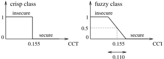
Figure 1: The crisp class and the fuzzy class for OMIB data
4 Experimental study
4.1 Datasets
We show in this section results obtained on 3 datasets: gaussian, twonorm and omib. Gaus-sian [5] is a synthetic database with 20000 ob-jects, 2 classes and 2 attributes. Each class corresponds to a bi-dimensional Gaussian dis-tribution. The first Gaussian distribution is centered at (0.0;0.0) and has a diagonal co-variance matrix, while the second one is cen-tered at (2.0;2.0) and has a non-diagonal co-variance matrix. There is an important over-lapping between the two classes. The Bayes classifier is of quadratic shape.
Twonorm dataset [3] is a database with 2 classes and 20 attributes. There are 10000 objects generated. Each class is drawn from a multivariate normal distribution with unit co-variance matrix. One class has mean (a,a,...a) while the other class has mean (-a,-a,...-a) where a = 2
√20. The optimal separating
sur-face (Bayes classifier) is an oblique plane, hard to approximate by the multidimensional rect-angles used in a crisp tree.
The omib2
database [11] is an electric power system database with 20000 objects that does a transient security assessment task. A three-phase short-circuit occurs in the system, nor-mally cleared after 155ms. The problem out-put reflects the system security state after the short-circuit fault occurrence. The input space is defined by 6 attributes representing pre-fault operating conditions of the OMIB system. The continuous output is defined as the fuzzy or crisp class of figure 1. The prob-lem is deterministic, that is why the Bayes error rate (the residual error) is null.
2
The acronym OMIB stands for One-Machine-Infinite-Bus system.
4.2 Protocol of experiments
Each database was split into a pool set, a pruning set P S and a test set T S. From the pool set, multiple q growing sets GS of the same size have been randomly chosen by sam-pling without replacement in order to build multiple models for each dataset. Table 1 presents the size of each set: pool set, grow-ing set, prungrow-ing set and test set for the three datasets. Each model has been grown on GS, pruned on PS, tested on PS, and refitted or backfitted on GS. In the results presented fur-ther q = 20 models have been averaged for the study of the global variance and q = 25 for the study of the parameter variance. The soft decision trees have been compared with CART regression trees and with ULG deci-sion trees (see [2] and [11]). CART and ULG trees were completely grown and then pruned. CART and SDT were trained for a regression goal (0/1 in the case of the crisp pre-classified datasets, µ(C) in the case of fuzzily classified ones). ULG was trained on a crisp classifi-cation goal, classes being converted into 0/1 class-membership degrees to compute bias, variance and mean-square errors.
Table 1: Datasets
Database Pool set GS PS TS Gaussian 14000 100 2000 4000 Twonorm 7000 300 1000 2000 Omib 14000 500 2000 4000
4.3 Comparing SDT bias-variance tradeoff with crisp methods tradeoff
The global variance and bias3
have been com-puted for each method for the GS size of ta-ble 1. Figure 2 shows for each dataset the proportion of bias and variance in the mean squared error (MSE) of each method: CART, ULG, fully grown (F), pruned (P), refitted (R) and backfitted (B) SDTs. We may notice the next aspects from these graphics: SDT in all its versions, improves accuracy with re-spect to a crisp tree, being regression or de-cision tree, SDTs reduce very much the vari-ance of crisp trees, pruning step succeeds to
3
What we will call further bias is in fact the relative bias of eq. (3).
leave slightly constant bias and variance quan-tities and refitting and backfitting steps in-crease variance of SDTs.
Figure 2: The proportion of variance and bias in the mean squared error
4.4 Variance and bias variation in terms of the model complexity We computed bias, variance and error quanti-ties for models of different complexiquanti-ties. The complexity of a tree model is given here by the number of its test nodes. Figure 3 displays the evolution of MSE, variance and bias with the model complexity, for twonorm database, for fully-grown CART and fully-grown SDT. For a crisp tree as CART, the evolution is the classic one: bias decreases and variance in-creases with the complexity. And there is a trade-off point where the mean squared error is the best and the corresponding complexity is the complexity of the right sized tree: about 8 test nodes. We expected to find the same type of curve evolutions for SDTs but the re-sult looks like this: the variance is almost con-stant and very low, the bias is the principal source of error, and the error always decreases with the model complexity. Thus, the more complex a SDT, the better the accuracy. As the figures show, we point out that we found the tradeoff point between bias and variance by scanning CART regression trees up to 25 test nodes complexity. Whereas for the SDT, models with up to 350 test nodes have been scanned and no such point has been found.
Figure 3: Evolution of MSE, variance and bias with the model complexity on twonorm dataset
4.5 Fuzzy versus crisp output definition
One very interesting property of our soft de-cision tree algorithm is that it can reproduce a classical crisp classification but also a fuzzy output when such a fuzzy membership degree to the class is given in the dataset. To show the potential of our method in this case, we have chosen a database where it was possi-ble to define a fuzzy output because we had the necessary knowledge about the problem: the OMIB stability problem. Figure 1 shows the definitions of both crisp and fuzzy classes. They are both defined based on a parameter called CCT, the critical clearing time of the disturbance, which may be interpreted as a degree of stability.
So if the objective is to classify situations with respect to the threshold of 155ms, we actually have two possibilities: either we build a (crisp or soft) tree directly with respect to the dis-crete 0/1 output, or we use the fuzzy output to build a tree and then discretize its output a posteriori.
Figure 4 represents the mean squared error
Figure 4: Crisp (left part) versus fuzzy (right part) class on CART and SDT results and omib database
for CART, fully grown (F), pruned (P), refit-ted (R) and backfitrefit-ted (B) SDTs, in the crisp output case definition and in the fuzzy output case. As we may notice, all the quantities, MSE, bias and variance, are much decreased by the use of fuzzy output, for all the algo-rithms. So, when a fuzzy output is available, it can thus be used to improve the accuracy of the algorithms.
4.6 Variance and bias as function of the growing set size
Figure 5 displays the evolution of MSE, vari-ance and bias with the growing set size on omib dataset for the backfitted version of SDTs. As expected, both bias and variance decrease with the growing set size. They are almost constant and equal quantities for medium and large sample sizes. The refitted version of the SDTs gives the same allure of the curves as the backfitted SDT for all the datasets investigated.
Figure 5: Evolution of MSE, variance and bias with the growing set size on omib dataset 4.7 Parameter variance
Some references [4] show that classical dis-cretization methods of decision trees
actu-ally lead to very high variance of the cutting point parameter, even for large learning sam-ple sizes. We studied the behavior of soft de-cision trees from this point of view by measur-ing the variance of the cuttmeasur-ing point param-eter in a test node of the tree: firstly, in the root node, and secondly, in the second level test nodes (at depth 2).
The procedure was like follows. For each growing set size, we built q trees (CART, ULG and SDT). For each of these trees we kept the αcutting point parameter of the root node of the tree given that was corresponding to the same attribute. Thus we obtained at most q parameters, since not necessarily all the trees have chosen the same attribute in the root node. We computed the variance on these pa-rameters.
Figure 6 displays the evolution of the cutting point parameter variance with the growing set size at the root node, for omib database and the fuzzy class definition for ULG decision trees, refitted (R) and backfitted (B) SDTs. For this dataset, all the trees have chosen nat-urally the same attribute in the root node. Due to the adopted fuzzy partitioning ap-proach, the chosen attribute in the root node of a non-backfitted soft decision tree and its α value will always coincide with the ones cho-sen in the root node of a CART regression tree. For this reason, the cutting point vari-ance is identical for CART and refitted SDT in the root node. Once backfitted, a soft deci-sion tree changes its thresholds in all the tree nodes, and thus also its parameter variance. One may observe from figure 6 that a non-backfitted soft decision tree, identically to a CART regression tree, presents less param-eter variance in the root node than a ULG decision tree. By backfitting, parameter vari-ance in a root node of a SDT increases with respect to the non-backfitted version. The ex-planation resides in the fact that by globally optimizing, the location parameters are not any more restricted to fall in the range [0,1] and therefore they are more variable with re-spect to the average.
By studying the parameter variance in the root node of a soft decision tree, we are not able to see the contribution of the fuzzy ap-proach of splitting to the parameter variance
Figure 6: Evolution of the parameter variance with the growing set size at the root node in a whatever internal test node. Thus, we did also an experiment where the structure of the SDT was fixed and the complexity was settled to 3 test nodes. The structure has been deter-mined with an ULG decision tree built with the whole dataset. We present here the study for omib fuzzy output dataset. We watched also the evolution of the parameter variance with the growing set size.
We may notice from figure 7 that CART, refit-ted SDT and backfitrefit-ted SDT do not seem to show a significant difference in their param-eter variance at the second level nodes, but they are definitely all more stable from this point of view than the ULG method. The conclusion of this study is that the reduction of the global variance of SDTs (with respect to CART) is not correlated with a reduction of parameter variance (with respect to CART). Thus, the fuzzy partitioning does not improve the parameter stability with respect to a crisp partitioning. On the other hand, a by product of our study is that we found that parameter variance of CART (and also SDTs) is smaller than that of ULG.
5 Conclusions
This paper studied bias and variance of soft decision trees. An important conclusion of our experiments is that the improved accu-racy of soft decision trees with respect to crisp decision and regression trees is explained es-sentially by a lower prediction variance. Thus, soft decision trees are indeed another tool for reducing variance, beside pruning and aggre-gation techniques. However, complementary
Figure 7: Evolution of the parameter variance with the growing set size at the second level nodes of a soft decision tree (depth 2), for omib fuzzy output database
studies [9] have shown that soft decision trees do not reduce variance as much as aggrega-tion methods do. We have pointed out also that the variance in soft decision trees is not influenced by the model complexity, in con-trary to the case of crisp trees which variance increases quickly with their complexity. We have also highlighted the possibility to exploit a fuzzy pre-classification of objects and shown that this may also very significantly improve accuracy. On the other hand, the parame-ter variance study shows that the reduction in prediction variance of a soft decision tree with respect to a crisp regression tree is not corre-lated with a reduction in parameter variance. However, the parameter variance of CART re-gression trees and soft decision trees is smaller than that of ULG decision trees.
References
[1] X. Boyen and L. Wehenkel. Automatic induction of fuzzy decision trees and its applications to power system security as-sessment. Fuzzy Sets and Systems, 102 (1999) 3-19.
[2] L. Breiman, J. H. Friedman, R. A. Olshen and C.J. Stone. Classification and regression trees. Chapman and Hall, New-York, 1984.
[3] L. Breiman. Arcing Classifiers. The An-nals of Statistics. Volume 26, Number 3, pages 801-849, 1998.
[4] P. Geurts and L. Wehenkel. Investigation and Reduction of Discretization Variance in Decision Tree Induction. In ECML 2000, Proceedings of 11th European Con-ference on Machine Learning, Barcelona, Spain, May/June, pages 162-170, 2000. [5] P. Geurts. Contributions to Decision Tree
Induction: Bias/Variance Tradeoff and Time Series Classification. PhD Thesis, University of Li`ege, Belgium, 2002. [6] C.Z. Janikow. Fuzzy Decision Trees:
Is-sues and Methods. In IEEE Transactions on Systems, Man, and Cybernetics - Part B: Cybernetics, Volume 28, Number 1, pages 1-14, February, 1998.
[7] C. Marsala. Fuzzy Partitioning Using Mathematical Morphology in a Learning Scheme. In Proceedings of the 5th Inter-national Conference on Fuzzy Systems, FUZZ-IEEE’96. pages 1512-1517, New Orleans, September, 1996.
[8] C. Olaru and L. Wehenkel. A complete fuzzy decision tree technique. Fuzzy Sets and Systems138 (2003) 221-254.
[9] C. Olaru. Contributions to Automatic Learning: Soft Decision Tree Induction. PhD Thesis, University of Li`ege, Bel-gium, 2003.
[10] A. Suarez and F. Lutsko. Globally Op-timal Fuzzy Decision Trees for Classifi-cation and Regression. In IEEE Trans-actions Pattern Analysis Machine Intel-ligence. Volume 21, Number 12, pages 1297-1311, December, 1999.
[11] L. Wehenkel. Automatic learning tech-niques in power systems. Kluwer Aca-demic, Boston, 1998.
[12] Y. Yuan and M.J. Shaw. Induction of fuzzy decision trees. Fuzzy Sets and Sys-tems 69 (1995) 125-139.