Deep-learning feature descriptor for tree bark re-identification

(1)

Deep-Learning Feature Descriptor for Tree Bark

Re-Identification

Mémoire

Martin Robert

Maîtrise en informatique - avec mémoire

Maître ès sciences (M. Sc.)

(2)

Deep-Learning Feature Descriptor

for Tree Bark Re-Identification

Mémoire

Martin Robert

Sous la direction de:

Philippe Giguère, directeur de recherche Patrick Dallaire, codirecteur de recherche

(3)

Résumé

L’habilité de visuellement ré-identifier des objets est une capacité fondamentale des systèmes de vision. Souvent, ces systèmes s’appuient sur une collection de signatures visuelles basées sur des descripteurs comme SIFT ou SURF. Cependant, ces descripteurs traditionnels ont été conçus pour un certain domaine d’aspects et de géométries de surface (relief limité). Par conséquent, les surfaces très texturées telles que l’écorce des arbres leur posent un défi. Alors, cela rend plus difficile l’utilisation des arbres comme points de repère identifiables à des fins de navigation (robotique) ou le suivi du bois abattu le long d’une chaîne logistique (logistique). Nous proposons donc d’utiliser des descripteurs basés sur les données, qui une fois entraîné avec des images d’écorce, permettront la ré-identification de surfaces d’arbres. À cet effet, nous avons collecté un grand ensemble de données contenant 2 400 images d’écorce présentant de forts changements d’éclairage, annotées par surface et avec la possibilité d’être alignées au pixels près. Nous avons utilisé cet ensemble de données pour échantillonner parmis plus de 2 millions de parcelle d’image de 64x64 pixels afin d’entraîner nos nouveaux descripteurs locaux DeepBark et SqueezeBark. Notre méthode DeepBark a montré un net avantage par rapport aux descripteurs fabriqués à la main SIFT et SURF. Par exemple, nous avons démontré que DeepBark peut atteindre une mAP de 87.2% lorsqu’il doit retrouver 11 images d’écorce pertinentes, i.e correspondant à la même surface physique, à une image requête parmis 7,900 images. Notre travail suggère donc qu’il est possible de ré-identifier la surfaces des arbres dans un contexte difficile, tout en rendant public un nouvel ensemble de données.

(4)

Abstract

The ability to visually re-identify objects is a fundamental capability in vision systems. Of-tentimes, it relies on collections of visual signatures based on descriptors, such as SIFT or SURF. However, these traditional descriptors were designed for a certain domain of surface appearances and geometries (limited relief). Consequently, highly-textured surfaces such as tree bark pose a challenge to them. In turn, this makes it more difficult to use trees as identi-fiable landmarks for navigational purposes (robotics) or to track felled lumber along a supply chain (logistics). We thus propose to use data-driven descriptors trained on bark images for tree surface re-identification. To this effect, we collected a large dataset containing 2,400 bark images with strong illumination changes, annotated by surface and with the ability to pixel-align them. We used this dataset to sample from more than 2 million 64 × 64 pixel patches to train our novel local descriptors DeepBark and SqueezeBark. Our DeepBark method has shown a clear advantage against the hand-crafted descriptors SIFT and SURF. For instance, we demonstrated that DeepBark can reach a mAP of 87.2% when retrieving 11 relevant bark images, i.e. corresponding to the same physical surface, to a bark query against 7,900 images. Our work thus suggests that re-identifying tree surfaces in a challenging illuminations con-text is possible. We also make public our dataset, which can be used to benchmark surface re-identification techniques.

(5)

List of Tables

1.1 Face recognition datasets . . . 10

1.2 Person re-identification datasets. . . 13

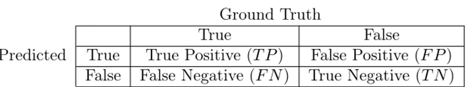
1.3 Confusion matrix . . . 32

1.4 Results with threshold example . . . 34

1.5 Ordered PR results example . . . 36

1.6 P@K results example . . . 36

1.7 Reference summary. . . 41

2.1 Existing bark datasets . . . 43

3.1 Hyperparameters grid search . . . 62

3.2 Hyperparameters chosen sample. . . 63

3.3 Saturation results . . . 64

3.4 Descriptors comparison results . . . 69

3.5 Generalisation across species results . . . 72

3.6 Negative examples experiment results . . . 75

3.7 Scoring methods mean comparison time . . . 76

3.8 Bag of Word Recall@K results . . . 77

A.1 DeepBark architecture . . . 88

(8)

List of Figures

0.1 Landmark recognition . . . 3

0.2 Bark self-similarity . . . 4

0.3 Qualitative matching performance . . . 5

1.1 Fab-Map 2.0 loop closure . . . 11

1.2 Urban park loop closure . . . 12

1.3 Local feature descriptor images comparison . . . 15

1.4 Neuron example . . . 18

1.5 Convolution operation . . . 19

1.6 Residual block . . . 20

1.7 ResNet performance . . . 20

1.8 Triplet loss learning . . . 23

1.9 N-pair-mc loss batch construction . . . 24

1.10 Classification in metric learning . . . 24

1.11 Softmax angular losses effects . . . 26

1.12 MVS dataset sample . . . 27

1.13 Domain generalization . . . 29

1.14 Example of scores with thresholds . . . 32

1.15 Example of scores with ranking . . . 35

2.1 Wooden frame example . . . 45

2.2 Bark surfaces examples . . . 47

2.3 Homography . . . 48

2.4 Transformation pipeline . . . 51

2.5 Keypoints registration . . . 52

2.6 Training patches examples . . . 53

2.7 Image signature . . . 56

2.8 Geometric Verification example . . . 57

3.1 Bark re-identification visualization . . . 59

3.2 Threshold lack of relativization . . . 61

3.3 Red Pine US-PR saturation . . . 65

3.4 Elm US-PR saturation . . . 65

3.5 Red Pine OS-PR saturation . . . 65

3.6 Elm OS-PR saturation . . . 66

3.7 OS-PR Curves descriptors comparison . . . 67

3.8 ROC Curves descriptors comparison . . . 68

(9)

3.10 US-PR Curves generalisation results . . . 71

3.11 OS-PR Curves negative examples results . . . 73

3.12 US-PR Curves negative examples results . . . 73

3.13 ROC Curves negative examples results . . . 73

3.14 Bag of Words size experiment results . . . 76

3.15 US-PR Curves negative examples results . . . 79

3.16 DeepBark score distributions . . . 80

3.17 SIFT score distributions . . . 81

A.1 Fire module . . . 86

A.2 ResNet-34 . . . 87

A.3 Red Pine ROC Curves saturation . . . 90

A.4 Elm ROC Curves saturation . . . 90

A.5 US-PR Curves descriptors comparison . . . 91

(10)

À ma fille Rose, pour qu’elle sache que tout est possible.

(11)

The good thing about science is that it’s true whether or not you believe in it.

(12)

Remerciements

L’achèvement de ce travail est le moment idéal pour moi de remercier tous ceux et celles qui ont contribué de près ou de loin à la réussite de ce projet. Aussi, je voudrais dire un merci tout spécial à ma conjointe, Valérie Côté, pour m’avoir supporté durant ce long et ardu projet. De plus, je tiens à remercier mon superviseur, le Professeur Philippe Giguère, pour ses nombreuses corrections et conseils, même si nous n’avons pas eu la chance de se croiser aussi souvent que nous l’aurions souhaité. Puis, j’aimerais dire un sincère merci à Marc-André Fallu, pour son amitié sans failles et son aide pour trouver des arbres bien identifiés pour ajouter à mes données. Il me faut aussi dire merci à Fan Zhou, pour son support essentiel dans mes derniers efforts de collecte de données. Finalement, merci au Fonds de recherche du Québec – Nature et technologies (FRQNT) pour le financement de ce projet.

(13)

Introduction

Nowadays, globalization is an undeniable fact, and it comes with lots of challenges. With the rise in the production and consumption of many goods and merchandise, transport logistics became a key challenge of our era. The tracking of objects such as merchandise thus became a necessary concept in many fields, and tracking within the supply chain is now a vital ele-ment of the Industry 4.0 philosophy. For example, in Cakici et al. (2011), they look at the radiology industry and evaluate the benefit of switching from an old tracking system using a barcode system and standard inventory counting practice to a new tracking system using Radio Frequency Identification (RFID) technology with a redesign of the business process to fully exploit the technology. They show that the new RFID system would allow a continuous review of the inventory and also reduce shrinkage by tracking expiration. According to Cakici et al.(2011), radiology practice faces difficult operational challenges that new tracking systems could alleviate and help make substantial savings. For Hinkka (2012), it goes without saying that RFID systems show real benefit for object tracking in the supply chain. This is why they focus on the reasons behind the slow adoption of such new tracking technology in supply chain management. Using a literature review, they notice that most published articles con-centrated on the technical problems related to RFID, while the problem currently preventing the adoption is more organizational or inter-organizational.

Closer to our subject, tracking objects or products in the forestry industry would consist in monitoring and managing the forest while tracking logged trees from the forest to their entrance in the wood yard. In Sannikov and Pobedinskiy (2018), they proposed a theoretical information system based on RFID to keep a continuous input of the forest state, measure the quantity of harvested wood, and track wood transportation. By building a network allowing communication between RFID device and receiver, they say it would enable the best decisions to be made and help switch from a manual forest management to a remotely automated process. Then inMtibaa and Chaabane(2014), assuming a forestry company already tags its resource with RFID devices, they propose a software system able to connect to an application layer (XML files and RFID tag). From there, the system can store and process raw data that become available through a web portal that provides both the business and client with easy access to reports and a traceability interface of the resource. According to Mtibaa and Chaabane (2014), such a system would allow companies to engage in product certification

(14)

and optimize the distribution of their raw material as well as the best location to keep their inventory.

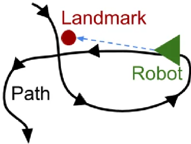
In the context of mobile robotics, localization is fundamental to enable the robot to move around in his environment in an informed way. In Hellstrom et al.(2009), they use multiple sensory receivers such as a laser scanner, a Global Positioning System (GPS), a gyro, a radar and the vehicle odometry in combination with their new path tracking algorithm developed to follow a learned path based on the steering command to make a 10 tonnes Valmet 830 forwarder follow a precise 160-meter long path. They tested their new algorithm on a Valmet 830 forwarder to simulate as much as possible autonomous wood forwarding in a forest en-vironment. However, the primary sensor they used to re-evaluate their vehicle position was their GPS system that was precise to 2cm in their control environment. As they mentioned themselves, GPS systems need a clear view of multiple satellites, have their accuracy sensitive to environmental conditions, and need a stationary receiver to correct recurrent bias. So, forests are a harsh environment where these flaws could prove critical for localization systems. This is why our research aims to provide a reliable localization method based on tree bark to be used as visual landmarks. The importance of landmarks in localization systems comes from their ability to make loop closure in algorithms such as Simultaneous Localization and Mapping (SLAM). In this algorithm, the robot moving in its environment detects interest-ing landmarks and then stores their descriptions associated with their location together in a database. This enables newly-seen landmarks to be compared with the ones previously seen in the database. When a newly detected landmark (referred to as A here) is matched with a previously-seen one (referred to as B), the assumed location that would be given to landmark A is then compared with the assigned location of the landmark B. This allows an evaluation of the error incurred by the distance travel since having seen the landmark B. That way, these landmarks enable the repositioning of the robot and the correction of the probabilistic map it is simultaneously building. Looking at Figure 0.1, we can see a simplistic example of a robot detecting a previously-seen landmark on his path that will allow him to readjust his map and position hypotheses.

In the work of Smolyanskiy et al. (2017), they present a micro aerial vehicle (MAV) system able to navigate a 1-kilometer forest trail autonomously. Their system uses a 3DR Iris+ quadcopter equipped with sonar and lidar to calculate altitude and velocity but relying on a single forward-facing Microsoft HD Lifecam HD5000 USB camera to calculate the MAV orientation and lateral offset from the forest trail while also detecting objects and obstacles on the trail. Thus, they use monocular SLAM to navigate and follow the current forest path that, in their experiment, did not need any loop closure, since they tested their system on trails without any intersection and 1 kilometer or less in length. Thus, they showed a high capacity to follow forest trails autonomously but would need a better re-localization system for longer trails with many similar path junctions. A great example of the usefulness of landmarks in a

(15)

Figure 0.1: Previously seen landmark recognized a second time by a mobile robot.

more complex path is inRamos et al.(2007). In their paper, they propose a system to detect, describe, and associate landmarks to improve the SLAM algorithm in an outdoor setting. This setting is interesting for us since it is an urban park populated by trees that they use as landmarks, among others. Their approach begins by using laser information to select a possible landmark region. Then, cropping the image from the camera to the proposed region, they classify the crop as a landmark or not. If the image patch is considered as a landmark, they make an appearance model based on the appearance described by a mixture of Gaussians, fused with the position information. Finally, to retrieve previously-seen landmarks, they compared the new appearance model with the ones that were stored using the gated nearest neighbor method. They compared their approach based on an estimated trajectory on a 1.5-kilometer-long path containing several loops using the GPS trajectory collected as ground truth. The two competitors were simple odometry and the standard EKF-SLAM method that both underperform compared to the proposed approach. However, their results still have room for improvement, and their outdoor environment being an urban park has a more sparse distribution of trees than what is expected in a forest. Moreover, using position information in the appearance model would not allow a robot to solve the exploration problem or recover from the wake-up or kidnapping problem common in mobile robotic.

To allow tracking or localization using trees, one must gather information from theses trees that are available all day and all year while displaying distinctive characteristics from one tree to another one. Thus, we chose to use images of tree bark as the source of information for its availability, but also because we suspect an inherent distinctiveness among tree bark, similar to the fingerprint of humans. From this, we designed a system using the standard pipeline of local feature descriptors to extract the distinctive representation inherent to a bark surface. Basing our approach on this typical pipeline will also allow us to use standard comparison

(16)

techniques on which we will rely for the data association step of our system. However, looking at Figure 0.2, we can see six images taken from three different bark surfaces that reveal the self-similarity of tree bark while making clear the effect of lighting variation. Indeed, bark texture induces significant changes in appearance when lit from different angles, and it is also important to note that scale and viewpoint variations considerably affect bark appearance too. So, to track trees or use them as landmarks in localization, one must be able to re-identify them and, in our case, make this re-identification based on bark images. In this thesis, we precisely explore this problem by developing a method to compare images of tree bark and determining if they come from the same surface or not.

Our main research objective can be summarized with the following question:

Is it possible to reliably recognize an individual tree with a visual

signature extracted from its bark?

1-a 1-b 2-a 2-b 3-a 3-b

Figure 0.2: In this figure, we can see 6 images taken from 3 different bark surfaces identified by the number 1,2,3. Letters a and b make the distinction between two images of a same surface. Comparing images from 1 to 3 shows the self-similarity of bark from different trees while comparing a and b images allows us to see the effect of different illumination angles.

Another assumption we made is that current hand-crafted local feature descriptors are not adapted to give invariant descriptions in the face of significant changes in illumination and viewpoint on bark images. But, new techniques introduced recently have the potential to learn this invariance. Since the advent of the Convolutional Neural Network (CNN) starting when Krizhevsky et al. (2012) won the ImageNet competition in 2012, these new artificial neural networks showed a high capacity to learn a non-linear function enabling unprecedented generalization and invariance. This is why, in this thesis, we propose to replace the description part of the standard local feature descriptor pipeline by a CNN trained on bark images to output invariant descriptions of bark images. A preview of the qualitative performance is

(17)

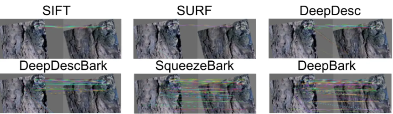
shown inFigure 0.3, which demonstrates the difficulty of dealing with tree bark and descriptors not tailored for it. However, a weakness of these deep learning networks is their tremendous need for useful quality data to learn efficiently. At the beginning of this project, this was indeed another difficulty with the absence of a dataset tailored to this problem. There are already-existing bark datasets such asFiel and Sablatnig(2010);Svab(2014);Carpentier et al.

(2018), for example. Still, these are geared towards tree species classification, and we not only need a bark dataset allowing bark instance retrieval. We need a dataset that enables direct physical correspondence between specific points in multiple images of the same bark surface.

Figure 0.3: Qualitative matching performance of different descriptors, for two images of the same bark surface. Every match shown in the image passed a geometric verification. Some false positive matches remain, due to the high level of self-similarity. Notice the great illumination changes between the image pair, a key difficulty in tree bark re-identification.

To this effect, we collected a dataset of our own, with 200 uniquely-identified bark surface samples, for a total of 2,400 bark images. With these images, we were then able to do bark instance retrieval. This was done by using one of the 12 images of a single bark surface as a query and use our description and data association algorithm to find the other 11 relevant images among all the other bark images used as a test set. The particular fiducial markers we took care to have in every image also provided us with the opportunity to produce a feature-matching dataset enabling the training of deep learning feature descriptors. With all this, we established the first state-of-the-art bark retrieval performance, showing promising results in challenging conditions. In particular, it surpassed by far common local feature descriptors such as Scale Invariant Feature Transform (SIFT) (Lowe (2004)) or Speeded Up Robust Features (SURF) (Bay et al. (2006)), as well as the novel data-driven descriptor DeepDesc(Simo-Serra et al. (2015)).

In short, our contributions can be summarized as follows:

• We introduce a novel dataset of tree bark pictures for image retrieval. These pictures contain specific fiducial markers to infer camera plane transformation.

(18)

bark images using standard neural network architectures and establish the new state of the art performance for bark re-identification.

• We show that bark surfaces are sufficiently distinct to allow reliable re-identification under a challenging context.

• We compare hand-crafted and deep learning methods on the bark re-identification task and show the necessity of the latter to achieve satisfactory results.

To efficiently understand our approach, the first chapter of this thesis gives the theoretical foundation we used and the current state of the art of the work related to our research. This background information will, for one, cover the subject of computer vision. More precisely, it will discuss the different tasks related to image retrieval along with several ways to describe images in a meaningful way and the useful measures to evaluate this kind of task. Then, an overview of concepts from machine learning about our project will be presented. Among these concepts are the CNN and the objective functions used to train them. We will also look at the latest work on Deep Learning descriptors and the recent papers working on the subject of bark images.

With this knowledge, we will then move toward the second chapter describing our data and methods. These two concepts will be mixed together. That is because we cannot speak of the composition of our dataset without going through the detail of the methodology to collect the said data. Also, any methods discussed in this chapter are closely related to our data, since they are designed to transform, describe or compare bark images from our dataset.

Then, after the theory and methods of the two first chapters, we present the results of our experiments and discuss them in length in chapter 3. To begin, we look at how to choose the optimal hyperparameters for a descriptor and investigate the impact of the size of the data used to train our Deep Learning local feature descriptors. After that, we compare the results of several descriptors being hand-crafted or learned and then examine the capacity of some of these learned descriptors to perform on tree bark species never seen in training. Following this, we produce our most convincing results by testing our best descriptor in a setting composed of bark images reduced in size while adding thousands of similar but unrelated bark images to try to reach the limit of the descriptive ability of our descriptor. Then, before ending this chapter, we evaluate the possibility to speed up the approach along with the possible decrease in performance and explore the distributions of the scores given by different image matching methods to discuss the problem of novel location identification.

Finally, we end this thesis with a conclusion, where we highlight some of the critical results we obtained and give a summary of the work that took us there. Subsequently, we take a moment to reaffirm our contributions before using them as a stepping stone, leading us to the future work it enables, while considering the weakness that should be addressed. Note that

(19)

this work can also be found among the published article of the 2020 Conference on Computer and Robot Vision (CRV).

(20)

Chapter 1

Background and related work

Before delving deep into our methodology, it is essential to start with the building blocks that led us there. In this chapter, we cover two broad subjects that ultimately take us to an efficient way to compare images of bark together. We begin by exploring the fields related to describing images and how to compare them. This mostly covers issues such as the formulation of image retrieval for different problems insection 1.1, the descriptors projecting whole images to compact descriptions insection 1.2, the descriptors giving invariant descriptions of interesting regions of images insection 1.3and the Bag of Words (BoW) technique to summarize multiple descriptions of interesting images regions insection 1.4.

Then, we discuss topics in machine learning relevant to our problem. For instance, we start by presenting a brief overview of Convolutional Neural Network (CNN) in section 1.5. Logically following this is metric learning in section 1.6, since it is essential to defined a well-suited learning objective for neural networks. After this, we discuss the multiple ways in which such a network can be trained to give a unique image description in section 1.7. Next, because of the loss of performance by learned descriptors when faced with unseen data from datasets too different, we cover the subject of domain generalization in section 1.8. We also review the latest works about bark and wood images relevant to our approach in section 1.9. Before we conclude this chapter in section 1.11, we go through different metrics useful to evaluating the numerous ways to describe and match images together in section 1.10. Works cited in this chapter have been aggregated in a table that is available at the end of the chapter, in

section 1.12.

1.1 Image Retrieval Formulations

Comparing two images directly by their content is useful for many computer vision applica-tions. However, it is generally a highly difficult problem (Wan et al.,2014;Neetu Sharma et al.,

2011). This is due in part to images having high dimensionality (the number of pixels times the number of color channels), making the semantic relevant content hard to extract. The

(21)

general case where having compact and semantically correct descriptions of images is useful, is the case of image retrieval. However, this task usually is constrained to specific problems, allowing the descriptions of images to focus on particular elements in images related to the constraint problem.

The problem of image retrieval can be defined as follow: given an image as a query, the goal is to find other images in a database that look similar to the query one. This was first addressed generically as Content-Based Image Retrieval (CBIR), which appears in conjunction with the consistent growth of images database that became harder to search as they grow, since it led to an increase in wrongly labeled images and that visually going through all images requires more time. In the beginning, searching images for this task was typically accomplished using more simple techniques such as PCA (Sinha and Kangarloo,2002) or color histogram based on HSV color model (Sural et al.,2002;Kaur and Banga,2013) and RGB color model (Neetu Sharma et al.,2011). There was also a discussion on the best way of ranking images by similarity to the query Zhang and Ye (2009) and the effect it has on the system performance. But, more recent works have started approaching the CBIR task with deep learning methods as in Wan et al. (2014);Arandjelovic et al.(2018), and there is also Zheng et al.(2016b) that use CBIR as the common ground to compare SIFT based descriptors and deep learning methods. For more in-depth information about CBIR, we strongly suggest to look into the survey made by Datta et al.(2008).

The problem was eventually tailored to specific domains, such as object recognition (Wang et al.,2017b;Sohn,2016;Wan et al.,2014;Zheng et al., 2016b;Yi et al.,2016;Rocco et al.,

2018;Sivic and Zisserman,2003;Lowe,2004;Bay et al.,2006). In this formulation, it consists of using a specific object image as a query to find images that contain similar objects, without necessarily showing the searched object exclusively. For example, in the well-known work of Sivic and Zisserman (2003), they showed qualitative results for objects such as a poster, a sign, or an alarm clock. For the poster, they retrieved 20 images, all containing the query object, but with only small variations of the object in the image. Then, for the sign, they retrieved 31/33 correct images and 53/73 for the alarm clock, but here again, it was the same object that needed to be retrieved. Object recognition becomes much harder when you consider retrieving different objects that are relatively similar. For instance, inSohn(2016), they tried to retrieve cars by model and flowers by species. This resulted in a recognition accuracy for cars of 89.21% and 85.57% for flowers. However, one could make the problem even harder by trying to cluster unseen objects together. For such a task, Sohn (2016) reported the best Harmonic Average of the Precision and Recall (F1) scores of 28.19% for online products, 33.55% for cars, and 27.24% for birds.

Another popular application is face recognition (Liu et al.,2017;Wang et al.,2017a,2018a,b;

Chopra et al.,2005;Schroff et al.,2015;Sohn,2016;Ming et al.,2018;Sun et al.,2014a;Parkhi et al.,2015;Wang and Deng,2018;Sun et al.,2016;Zhang et al.,2014;Taigman et al.,2014;

(22)

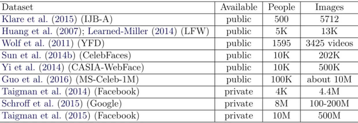
Sun et al.,2015;Taigman et al.,2015;Sun et al.,2014b). In this case, the goal can either be i) to correctly classify the identity of a person based on his face image or ii), taking two different images of a face and correctly assigning a label to the two images as being the same person or not. With the recent explosion of data and the easiness of keeping memories of people with images, the field of face recognition made a quick progression toward high performance. We see this phenomenon with companies such as FaceBook that built a dataset with 4.4 million labeled faces from 4,030 people inTaigman et al.(2014). They used a CNN and a face alignment technique to achieve 97.00% accuracy on the known benchmark Labeled Faces in the Wild (LFW) (Huang et al.,2007;Learned-Miller,2014) and 91.4% accuracy on the YouTube Faces DB (YFD) (Wolf et al.,2011) benchmark. Following this, Google inSchroff et al.(2015) worked with a dataset of 8 million identities, totaling 100-200 million images. With this, they achieve a remarkable 99.63% accuracy on LFW and 95.12% accuracy on YFD, without using anything other than a CNN. However, this dataset size is a challenge to manage on its own. This is why Facebook in Taigman et al. (2015) also worked on how to deal with such large datasets. For this, they made a new dataset containing 10 million different people with around 50 images each, giving roughly 500 million images. They reported a score of 98.0% on the verification task of LFW, which is more difficult than the recognition task. They obtained this score with a single network compared toSun et al.(2014a) who achieved 99.15% using an ensemble of hundreds of CNN in combination with information from the LFW images. With all the work in face recognition, we added Table 1.1 to give a better overview of the type of datasets available for this task.

Dataset Available People Images

Klare et al. (2015) (IJB-A) public 500 5712

Huang et al. (2007);Learned-Miller(2014) (LFW) public 5K 13K

Wolf et al.(2011) (YFD) public 1595 3425 videos

Sun et al. (2014b) (CelebFaces) public 10K 202K

Yi et al. (2014) (CASIA-WebFace) public 10K 500K

Guo et al.(2016) (MS-Celeb-1M) public 100K about 10M

Taigman et al.(2014) (Facebook) private 4K 4.4M

Schroff et al. (2015) (Google) private 8M 100-200M

Taigman et al.(2015) (Facebook) private 10M 500M Table 1.1: Table adapted from Guo et al.(2016). Standard datasets used in face recognition tasks. The number of different identities available in each dataset is the people column, and the total number of images is in the column images. However, the critical aspect is the availability of these datasets provided by the column Available, which depicts the advantage of large companies with their large datasets kept private.

In some other cases, the formulation was used for visual scene recognition (Yi et al., 2016;

Rublee et al., 2011; Alcantarilla et al.,2012; Calonder et al.,2010;Arandjelovic,2012). For the latter, the important aspect is to take an image depicting a certain scene such as a beach, a parking lot, or a forest and retrieve images showing the same kind of scene (but importantly,

(23)

not necessarily the same location). In mobile robotics, image retrieval is often used to perform localization. In this field, it is known as Visual Place Recognition (VPR) (Jain et al.,2017;

Zheng et al.,2017;Wan et al.,2014;Arandjelovic et al.,2018;Zheng et al.,2016b;Sunderhauf et al., 2015; Cummins and Newman, 2008, 2009; Turcot and Lowe, 2009; Li et al., 2010;

Rocco et al., 2018; Ramos et al., 2007). There, the objective is to determine if a location has already been visited, given its visual appearance. The robot could then localize itself by finding previously-seen images which are geo-referenced. This leads us back to the concept of SLAM and the associated problem of loop closure initially discussed in the introduction. However, we did not talk about the difficulty of such a task. An order of magnitude of the problem is provided by the Figure 1.1fromCummins and Newman(2009), which depicts the loop closure in red on a 1,000 km dataset. By comparing their ground truth in a) with the detected loop closure of their algorithm in b), we see that such a long road will inevitably exhibit difficult places to recognize visually. Also, we can look at Figure 1.2 to evaluate the improvement in localization moving from simple odometry to SLAM algorithm with visual landmarks, passing by standard EKF-SLAM. Nonetheless, on the right side of the figure where visual landmarks are used, we can still see some errors. It is worth noting that the trajectory is only 1.5 kilometers and is located in an urban park, which proves less difficult than other environments such as a dense forest or a snowy landscape where there is a lot of self-similarity in the scenery.

Figure 1.1: Figure taken from Cummins and Newman (2009). This figure shows a 1,000 kilometers trajectory with loop closure in red. The (a) panel provides the ground truth, and the (b) panel provides the detected loop closures by the Fab-Map 2.0 algorithm. They correctly detected 2,189 loop closures and predicted six false positives. This gave them a 99.8% precision at 5.7% recall. In the original caption, they mentioned that the long section with no loop closure detected is a highway at dusk.

In the area of video surveillance, the problem of Person Re-Identification (Person Re-Id) con-sists of following an individual through several security camera recordings (Hermans et al.,

2017;Zheng et al., 2017,2016b;Gray et al., 2007;Zheng et al.,2016a, 2015;Li et al.,2014). This technique implies to learn a function that maps multiple images of an individual to the

(24)

[a] [b]

Figure 1.2: Figures taken from Ramos et al. (2007). In each case, the blue line shows the estimated trajectory, and the green line represents the estimated ground truth using GPS information, which is not available in some areas of the urban park. In the top part of [a], the blue line is estimated using only odometry, and in the bottom part, we have an estimate using the standard EKF-SLAM. In [b] is the trajectory predicted by the algorithm using visual landmarks proposed byRamos et al. (2007). We can see that the proposed method improves a lot over the two other methods, but small errors are still visible, and the trajectory used could be more difficult.

same compact description, despite variation of viewpoint, illumination, pose, or even clothes. This way, if the description is unique for each individual and invariant to change in appearance, person re-identification can then retrieve a single person by computing the same description for this person across multiple cameras despite changes in view angle and different people being present. One of the standard datasets tailored for this task is the viewpoint invariant pedestrian recognition (VIPeR) dataset presented in Gray et al. (2007). However, it only contains 632 image pairs of pedestrians with variations only in viewpoint. By today’s stan-dard, this dataset is quite small with its total of 1264 images, but since then, larger datasets have appeared, and the most common are shown in Table 1.2. Numerous works have used these datasets as benchmarks. One of these is Zheng et al.(2017), who used a CNN trained with multiple objectives to achieve a rank-1 accuracy of 83.4 in the single-shot setting of the CHUK03 (Li et al.,2014) dataset. On the Market-1501 (Zheng et al.,2015) dataset, they

(25)

re-ported a mean Average Precision (mAP) score of 59.87 in the single query setting and a score of 70.33 in multi-query setting. More recently, better results have been reported by Hermans et al. (2017) on the CHUK03 and Market-1501 dataset, but also on the MARS (Zheng et al.,

2016a) dataset. For CHUK03, they achieved a rank-1 accuracy of 87.58 in a single-shot setting. On the Market-1501, they obtain a mAP score of 81.07 and 87.18 in single and multi-query respectively, and lastly, they reached a mAP score of 77.43 on the MARS dataset. It is clear that person re-identification is undergoing a rapid progression in performance during recent years, but one can also see that there is still room for improvement when looking at the latest results.

Dataset pedestrians images

Gray et al. (2007) (VIPeR) 632 1264

Li et al. (2014) (CUHK03) 1,360 13,164

Zheng et al. (2015) (Market-1501) 1,501 32,668

Zheng et al. (2016a) (MARS) 1,261 1,191,003

Table 1.2: Standard datasets used for the person re-identification task. The column pedestrian shows the number of different identities available in each dataset, and the total number of images is in the column images. These datasets are also in ascending order of apparition from top to bottom. We can see the growth in data following the passage of time.

1.2 Global Descriptor

In the early days of image retrieval systems, the first techniques to describe images relied on the complete image’s properties to perform correspondence. Making histograms from colors as in Neetu Sharma et al. (2011), for instance, can give some mildly reliable information about the image content. For example, an image with a predominance of blue might be an image of the sky or the sea, while an image mostly green will probably contain forests or vegetation. However, this information is not enough to precisely characterize an image and can at best allow the association of images with a loosely similar theme. Then, one can also look into Hue-Saturation-Value (HSV) color format (Sural et al.,2002;Kaur and Banga,

2013) to extract information more robust to illumination changes. In the work of Sural et al.

(2002), they used the HSV format to categorize pixels as a specific color if the saturation is low or, if it is high, for instance, as a black or white pixel. This is done to allow the decomposition of images using histograms and segmentation in a more relatable way to how humans perceive light. Another way to globally describe images is to view them for what they are in computer science: matrices. Then, using linear algebra, we can characterize images by extracting their eigenvectors. However, this is not readily applicable for images within a dataset, without further processing. For this reason, Sinha and Kangarloo (2002) further constrained their problem by employing dimensionality reduction with Principal Component Analysis (PCA) to compare images based on the variation of their principal components.

(26)

Nonetheless, these techniques may give too much importance to background information, often relating to location and drown small but crucial visual information such as objects or persons, as explained inDatta et al.(2008). Also, they are weak against changes in viewpoint, as mentioned inLowry et al. (2016).

Since then, other methods have been developed to describe images globally that broadly differ from the one previously mentioned. First, there is the BoW method (Sivic and Zisserman,

2003) that globally describe an image by summarizing the set of all descriptions produced by a local feature descriptor such as SIFT or SURF. There is also a growing interest in using CNN trained on classification tasks to extract a single vector representing a whole image (Wan et al.,

2014;Sunderhauf et al.,2015). However, we will not discuss these methods here, because they are the subject of another section.

1.3 Hand-Crafted Local Feature Descriptor

Instead of taking the whole image and calculating a global description as a form of summary, local feature descriptors aim at representing an image through a collection of descriptions taken from smaller regions of the image. For these descriptions to be relevant, the small image regions they describe must be a distinctive or meaningful part of the image. The first step in using such a descriptor is to find the location of interesting regions of the image. In the context of local descriptors, these regions are specifically referred to as keypoints. These keypoints are found using a keypoint detector, which looks through an image, searching for strong gradients as in Lowe (2004) or searching for corner using pixel intensity as in Viswanathan (2011);

Rosten and Drummond (2006). This change in gradient or pixel intensity correlates strongly with edges and corners in an image, which makes them reliable points. The advantage of this technique is that if we can reliably find the same keypoints in an image, we can obtain a nearly invariant representation of the image while mostly including only meaningful parts of it. Once the keypoints are found, the descriptor is then used to describe all of the keypoints surrounding regions following an algorithm devised by an expert. This is the reason why they are called hand-crafted.

The goal of a local descriptor is then to summarize the visual content of an image patch taken at the location of a keypoint. This enables a comparison between images based on feature correspondence, as seen inFigure 1.3. The ideal descriptor is a) compact (low dimensionality) b) fast to compute c) distinctive and d) robust to illumination, translation and rotations. These are important qualities for local feature descriptors, because the number of descriptions to be made in an image can total over 2000, which can be costly in computation and memory space. A widespread approach of hand-crafted methods to describe image patches is often to rely on histograms of orientation, scale, and magnitude of image gradients, as in SIFT (Lowe,

(27)

Figure 1.3: Figure taken from Arandjelovic (2012). It compares the descriptors based on the number of matches retained and the localization quality of the keypoints that have a match. On the left is the query image, and on the right is the image compared with the estimated correspondences. It shows that RootSift offers descriptions that are more distinctive and allow better matching of more locations.

alleviate the computation cost (Calonder et al.,2010;Rublee et al.,2011) or simply trying to increase the performance (Alcantarilla et al.,2012;Arandjelovic,2012).

1.4 Bag of Words

The Bag of Words (BoW) is a discretized representation of all the information provided by a local feature descriptor. It is calculated from the list of descriptions V generated by the descriptor on an image, which are lists of vectors of reals. The advantage of such a technique against directly using V , is the speed at which two BoW can be compared. Since BoW are discretized summary of a list of descriptions extracted from images, this allows for a fast comparison of these images, which is useful in large datasets. An excellent reference to follow is Manning et al. (2008) in section 6.2, which we explain next.

The idea of BoW in computer vision has been borrowed from the information retrieval domain. As its name suggests, the BoW is essentially a multiset (bag) of every word in a document.

(28)

This serves as a summary vector representation of a complete document, using the count of each word present in this document. In computer vision, the idea of words has been extended to the concept of visual word in an image. However, visual words are not defined in advance as words, instead, they represent a cluster composed of similar visual features. These visual features are small parts of an image considered as informative, such as edges, corners, repetitive structures, or any meaningful pattern in an image. This means that visual words must be defined using clustering methods such as the K-mean clustering algorithm from a large set of visual features extracted from available images. Once we clustered our set of visual features into a fixed number k of clusters, we end up with k visual words that become what is known as a visual dictionary voc of size k. More formally, the voc calculation is done by using a keypoints detector and descriptor to extract all the keypoints descriptions available in a subset of the dataset we want to use for evaluation. Then, these descriptions, which become our visual features, can be clustered to build our voc. Finally, we can calculate a BoW representation of unseen images by extracting their visual features and clustering them into our voc, giving us the count of visual features for every visual word in an images, as we explain below.

Once we have a relevant voc for our dataset, we can calculate the BoW representation of an image I. To do so, the Term Frequency (TF) of each visual feature in I must be determined. The equation for a single TF is written as:

T F = nz

|V |. (1.1)

Here, V is the list of descriptions previously computed for the image I using the chosen detector and descriptor pipeline. Then, nz is the number of descriptions from V being clustered with

the visual word z, and |V | is the number of descriptions in our image. Doing this for every visual word in our voc gives a normalized BoW representation of I, with the same dimension of the voc.

However, some visual words may be present in almost every image of a dataset due to their repetitive nature. For instance, a dataset taken in the street of a city may show street lights in every image, so detecting them will not help to differentiate two images coming from different places. To mitigate this problem, one can calculate the Inverse Document Frequency (IDF) of a visual word from the subset T of our dataset. This enables the adjustment of the BoW by weighting each visual word according to their presence ratio in T . This way, it mostly ignores visual words present everywhere while giving more importance to the less present ones that are more informative. The IDF of a single visual word is defined as:

IDF = log|T | mz

. (1.2)

The numerator term |T | corresponds to the number of images in the subset T of the chosen dataset, which we divided by the total number of images mz in T having a least one description

being clustered with the visual word z. Once every TF in the BoW of an image is weighted by his corresponding IDF, we then obtain a more distinct representation of our image I.

(29)

1.5 Convolutional Neural Network

One of the critical developments in computer vision is the Convolutional Neural Network (CNN). The first successful application of CNN was for hand-written digit recognition (Lecun et al.,1998). They began by building a large set of hand-written digits known as the MNIST dataset from the larger NIST dataset. During their experiment, they used their LeNet neural architecture to show the advantage of CNN against other methods such as K-NN classifier, SVM, and fully-connected neural network. However, the usage of CNN did not take on initially, despite its vast potential. The interest for CNN-like architectures only took off when it was first used in the ImageNet (Deng et al.,2009) competition, with AlexNet (Krizhevsky et al.,

2012). In this work, they reported a significant winning margin against the best competitor. They succeeded in significantly reducing the current error margin with their AlexNet model trained using a smart GPU implementation of the convolution operation. They also discussed the use of drop-out, non-saturating neurons, and max-pooling that helped achieve their results. It is with this demonstration that the true capability of CNN had been unveiled.

Neuron

This capability comes from a fundamental building block called artificial neuron. The connec-tionism approach of artificial intelligence uses these neurons as their main inference engine. When grouping them in layers and then stacking multiple layers together, it becomes what is referred to as deep neural networks. These networks are part of the subset of machine learning, known as deep learning, which includes CNNs.

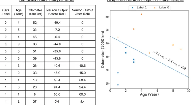
Neurons are based first on a linear equation that possess a parametric weight for each input it receives plus a weight bias. This is followed by a non-linear function referred to as an activation function. Being non-linear is a crucial component of the neuron, because it enables multiple representations of an input that would be impossible otherwise. Also, if one would stack several layers of neurons together without non-linearity, the network could then be reduced to a single linear operation. The standard activation function currently used in deep neural networks is the Rectified Linear Unit (ReLU) (Nair and Hinton, 2010). This function is defined as the maximum between the input and 0: max(x, 0). A neuron using a ReLU activation becomes a pattern detector that outputs a positive number only when the input satisfies a particular input pattern. This is demonstrated in Figure 1.4, which shows an example of a neuron receiving five inputs describing a car. The neuron only activates when a car is not too old and shows little mileage. In this toy example, the network might be trying to predict which car a potential client might buy, and this particular neuron learns to respond when a car is relatively new, since this is what a client might want. A latter neuron can discriminate more complex patterns based on the recognized patterns of the preceding network layer and so on so forth.

(30)

Figure 1.4: Visualization of the neuron discriminating old cars with lots of mileage. Thus, we can see that this neuron will respond to cars that seem relatively new, based on age and mileage. This is based on a toy example where a model tries to predict preferred cars (label 1).

CNN filter

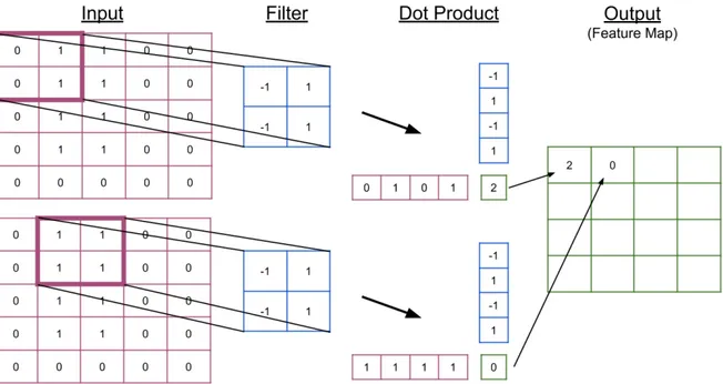
CNN filters are the CNN neuron, but the pattern they search has been specialized for the 2D grid-like arrangement of images. So to find these patterns, CNNs use the convolution operation that essentially multiplies a matrix (the CNN filter) with a corresponding image patch taken at every pixel position. The first two steps of this operation can be seen in

Figure 1.5. We can also understand that the filters used in a CNN layer are no more than another linear equation evaluated at a set of pixels. One advantage of this operation is that the matrix format allows us to take into account the spatial structure of an image in which the smaller pattern resides. The other advantage of the convolution is that parameters are shared across image locations, making a single filter capable of finding a recurrent pattern in the image wherever it is. The last significant difference between a fully-connected layer and a CNN one is the output. Where a fully-connected layer gives a new array of features, the CNN

(31)

layer will instead output a feature map. When a single filter is convolved against an image, the repeated matrix multiplication produces a result for every pixel position that needs to be kept in the same two-dimensional position to avoid losing the coherence of the image. The resulting matrix visible in Figure 1.5 is an example of such feature maps. The final output of a convolutional layer is then a 3-dimensional tensor that is the concatenation of all the outputted feature maps, since each filter of a CNN layer produces such a feature map.

Figure 1.5: Visualization of the convolution operation. In this figure, we can see that the filter is multiplied element-wise at each pixel position, and is equivalent to doing the dot product between two vectors. Note that for brevity, we omit the addition of a weight bias after the dot product operation.

CNN architecture

A network is typically defined by a particular arrangement of blocks, such as convolution layers, number and size of filters, max pooling, etc. Architectures greatly influence the results obtained by deep learning networks. Consequently, they are designed to induce a favorable bias for the task at hand. For example, the simple fact of using convolution operations causes a bias that makes deep networks such as CNN more efficient on images.

One architecture that showed outstanding performance and that is available under different sizes is the ResNet (He et al., 2016). This design intention was to transform the neural network such that it learns the residual of an identity function, at each layer. It comprised a residual block, which is composed of two convolutional layers, which are added to the original input via a skip connection, as displayed in Figure 1.6. This made every subsequent residual block processing a mix of the original input with the features obtained from the preceding blocks. Moreover, the skip connection enables the gradient coming from the final

(32)

prediction error to be easily back-propagated to the first layer of the network. This greatly facilitates the training of ResNet-like networks and increases the design flexibility in terms of the number of layers, which in turn gives better results when using more layers, as reported in Figure 1.7. Consequently, many ResNets models are publicly available in common deep learning framework. The complete architecture of a ResNet with 34 layers can be seen in

Figure A.2.

Figure 1.6: Residual block, as presented in He et al. (2016). The F (x) function is defined by the two-weight layers and the ReLU activation function. These weight layers can be any kind of layer, such as convolutional ones. The improvement made compared to traditional networks comes from the addition of the original input x to the output of F (x). This addition between input and output helps to back-propagate the gradient. Also, this forces each block to learn the residual of an identity function.

Figure 1.7: ResNet performance as presented in He et al.(2016). These results were obtained using single-models on the ImageNet validation set and are reported as error rates (%). The number beside ResNet networks indicates the number of layers. From this, we can see a clear improvement following the increase in layers.

(33)

Another interesting CNN architecture variation is SqueezeNet (Iandola et al.,2016). In their work, they proposed to focus on the sheer number of parameters in SqueezeNet, instead of trying to improve raw performance. For a quick comparison, the small 18-layers ResNet has 11,689,512 parameters, while the SqueezeNet 1.1 version only has 1,235,496. This gives a nine-fold reduction of the number of parameters while keeping an accuracy similar to AlexNet. Such a feat was achieved with a new CNN building block named Fire Module, and is depicted in Figure A.1. It was designed to employ three strategies aiming at reducing the number of parameters needed for convolution, while keeping the highest accuracy possible. Their first strategy was to reduce the number of costly 3x3 filters by replacing a portion of them by smaller 1x1 filters. Then, since filters are designed to be applied on every feature map simultaneously, the Fire Module incorporates a layer of 1x1 filters squeezing the number of feature maps before using 3x3 filters on it, thus reducing the depth of the 3x3 filters. Finally, the last strategy was to delay the feature map resolution reduction in the network, considering that He and Sun(2015) have shown that such a strategy can improve performance.

1.6 Metric Learning

As discussed in section 1.1, deep learning is now an essential component in image retrieval. This mostly spurs from the fact that deep learning networks can learn complex and non-linear representations that allow high-dimensional input to be easily classifiable in a non-linear fashion. This, in turn, means that a deep neural network can project its inputs to a compact representation that is meaningful for the task at hand. For a deep neural network to solve the ImageNet challenge, for example, it had to learn a projection that could take millions of images and send them to a small and meaningful representation to be linearly classifiable in 1000 categories. This hard task generated deep models able to encode a large array of complicated images features from the real world into low dimensional vector representations. These models essentially became global image descriptors and began to be used as such in problems such as VPR (Sunderhauf et al.,2015).

However, certain problems need more than having linearly-separable and meaningful vectors for an arbitrary number of classes. For example, in face recognition, we need to differentiate two distinct persons by their faces. Consequently, a deep model which could accomplish this for two, a hundred or even thousands of faces may not be enough for an application dealing with millions of unseen peoples. This becomes a problem about instance-level representations instead of classes and is useful, among other things, for instance-matching problems. Thus, the objective of a deep learning model used for instance retrieval, should be about making instance representations as distant from each other when different instances are involved, while keeping variation of the same instance as close as possible. This problem is well-adapted to the paradigm known as metric learning. More specifically, metric learning aims at designing a loss function that would allow a metric to be learned in the representation space. Below,

(34)

we discuss recent progress made in metric learning insubsection 1.6.1. As classification losses provide good performance and greatly impact the representational power of deep models, we also discuss the use of theses losses in the metric learning setting insubsection 1.6.2.

1.6.1 Metric Loss Contrastive Loss

Distance metric learning is an approach that tries to learn a representation function to be used with a distance function d() between data points x. For example, we have a dataset S of labelled data (x, y) ∈ S with x being an example and y its class label. We also have a function f which outputs a vector f(x) ∈ Rd. In metric learning, the goal is to learn this function f to minimizes the distance between the feature vectors, d(x1, x2) = ||f (x1) − f (x2)||22, when both

data points x1 and x2 belong to the same class y1 = y2. It must also maximizes the distance

when x1 and x2 belong to different classes (y1 6= y2). This function f can then be used to

compare unseen examples similar to the ones in S. The loss doing this base scenario can be found in Hadsell et al. (2006); Chopra et al. (2005); Simo-Serra et al. (2015); DeTone et al.

(2018) and is called the contrastive loss, as defined here: L(W, Y, X1, X2) = (1 − Y ) 1 2(Dw) 2_{+ (Y )}1 2{max(0, m − Dw)} 2_. _(1.3)

In equation1.3, Y is a label directly stating if a pair of examples (X1, X2)are similar (Y = 0)

or not (Y = 1). W are the parameters of Dw that represent the distance function to be

learned. This function should minimize the distance when Y = 0 and maximize to the extent of a margin m when Y = 1.

Triplet Loss

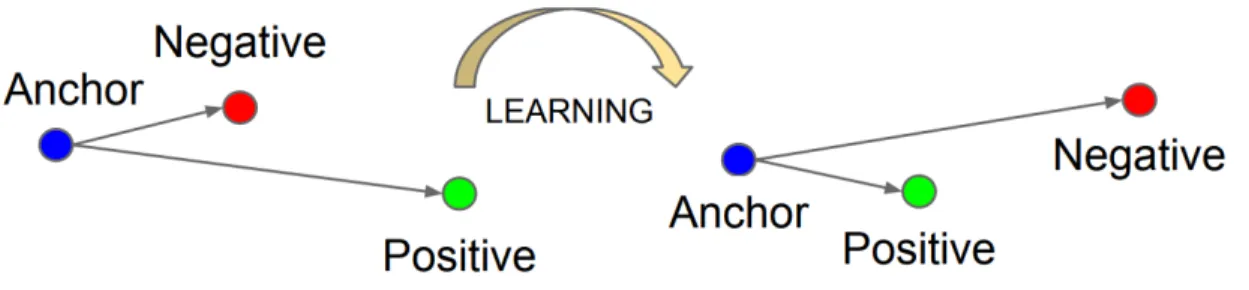
Instead of bringing together similar pairs in the embedding space as much as possible, one can try to make the inter-class variation larger than the intra-class one in the embedding space of the descriptor, as described in Figure 1.8. This is called the triplet loss (Schroff et al.,2015;Ming et al.,2018;Arandjelovic et al.,2018;Li et al.,2017a). It is computed from three examples (hence its name), made of an anchor example x, a positive example x+_{, and a}

negative example x−_{. They are used to learn the following inequality:}

||f (x) − f (x+)||2₂ < ||f (x) − f (x−)||2₂. (1.4) This inequality can then be translated to an actual loss:

L(x, x+, x−) = m + ||f (x) − f (x+)||2₂− ||f (x) − f (x−)||2₂. (1.5) This Equation 1.5 pushes the distance between a positive x+ _{and a negative x}− _{pair further}

than the selected margin m. In the case of Wang et al. (2017b), they tried to improve the triplet loss by adding constraints based on triangle geometry, to ensure the proper movement of the triplet sample in the embedding space during learning.

(35)

Figure 1.8: This figure shows the result after learning the representation with the triplet loss. The goal of this loss is to make the distance in representation space between two points of the same class A (here the anchor and the positive) smaller than the distance between a point of class A and a point of a different class such as B (here the negative) by a certain margin. It will cluster points of the same class together while assuring a certain margin with other classes. This figure was taken from Schroff et al. (2015).

Triplet Loss Variant

Sohn(2016) created the N-pair-mc loss to improve upon the idea of moving one pair of positive examples away from the negative pair one at the time. There, the goal is to use an ingenious batch construction process, shown inFigure 1.9, to enable the comparison of one positive pair x, x+ with multiple negatives examples xi at a time. This loss is expressed as:

L({x, x+, {xi}N −1i=1 }; f ) = log(1 + N −1

X

i=1

exp(f>fi− f>f+)), (1.6)

with the N-pair-mc loss using the N − 1 negatives examples xi to move the positive pair

x, x+ away from every one of them. This has the critical benefit of avoiding that the pair x, x+ of a triplet (x, x+, x−_i )gets closer to an unseen negative example x−_j during a mini-batch learning update. Also,Hermans et al.(2017) showed that comparing the hardest positive pairs (dissimilar examples that should be similar) with the hardest negative pairs (similar examples that should be dissimilar) in a mini-batch can lead to even better results in some instances.

1.6.2 Classification Loss

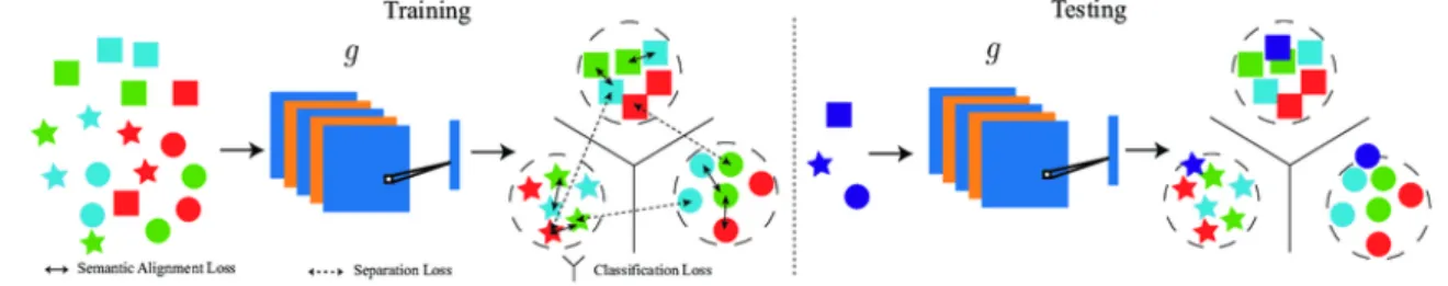
With the loss previously explained insubsection 1.6.1, our function f(x) has generally learned to output representation easily comparable in Euclidean distance. The kind of representation learned when classifying with the cross-entropy loss is different, but still relies on a form of distance. A cross-entropy loss is normally used to learn the categorization of instances of a pre-defined problem by transforming the final output of a network into a set of class proba-bilities. However, this final output given by the network can be seen as the non-normalized angle between the last layer and the input it receives, as explained in Figure 1.10. When considering this angle as a distance, it makes the penultimate layer representation learned with classification useful in metric learning, as we explained below.

(36)

Figure 1.9: This figure shows the ingenious batch construction process used by the N-pair-mc loss to reduce the number of evaluations needed to transform each example in their vector representation. In a), we can see the standard Triplet loss that chooses N triplet for a batch, resulting in the need for 3N evaluations. In b) is a naive selection of examples for a (N + 1)-tuplet loss batch, resulting in the need for (N + 1)N evaluations. Finally, in c), we can see that to reduce the number of evaluations needed, the N-pair-mc loss selects only N positive pairs of examples. Then, it used half of these pairs as the negative examples to create N (N + 1)-tuplet, reducing the total number of evaluations to only 2N. This figure was taken from Sohn (2016).

Figure 1.10: The dot product of the input representation at the n − 1 layer and the weights of the last layer n can be considered as the non-normalized angle between them. This angle can thus serve as a distance and lead us to think of the input representation given by the n − 1 layer as a representation learned using a distance. The cross-entropy loss indirectly does this by making examples of the same class have similar angles and make classification useful in metric learning.

Cross-entropy Loss

(37)

two distinct instances of a dataset, it may not be mandatory to directly enforce a distance between every instance. Instead, Sun et al. (2014b) use a cross-entropy loss to learn the classification of 10,000 different faces. Having many classes forced their CNN model to learn a function that output sufficiently-detailed representation before the last layer to be successfully used in a face verification task.

Similarity Loss

Even if classification can be used for metric learning, it is not the most suitable loss for verification, i.e., to decide if an unseen image pair is considered the same or not. To tackle this problem, a verification loss using binary cross-entropy (Xufeng Han et al., 2015; Sun et al., 2016) was developed to directly output the probability of two images being the same (0 different, 1 same). If we consider this probability as a distance, this loss becomes similar to the contrastive loss by pushing the distance between similar examples to 1 and different examples to 0.

Multi Loss

With the great success of losses based on learning distances and the significant power of classification, it is not surprising to see that this led to experiments which combined losses to improve over one another. In Sun et al.(2014a,2015), they trained their network by carrying out classification and using the contrastive loss at the same time. Similarly, Parkhi et al.

(2015) used a cross-entropy loss in conjunction with the triplet loss. In the case of Zheng et al. (2017);Taigman et al. (2014); Taigman et al.(2015), they combined classification with a similarity loss objective using binary cross-entropy. With all of these methods, Wan et al.

(2014) made a comparison of a pre-trained network on ImageNet with the same network fine-tuned on similar data to the test set using either a cross-entropy loss or a triplet loss. They concluded that a pre-trained network while offering good results, can have its performance significantly boosted by fine-tuning it with either loss.

Angular Loss

Since the performance shown by a cross-entropy loss is still relevant, some people started to address one of its disadvantages, namely the lack of proper decision boundaries. Liu et al.

(2017); Wang et al. (2017a, 2018a,b) alleviated this problem by modifying the softmax to incorporate an angular margin that must be overcome by the network to classify an example correctly. This problem can be seen in Figure 1.11, which also depicts the effect of adding a margin in the softmax classification loss in either the non-normalized vector space or the l2

normalized vector space.

1.7 Learned Local Feature Descriptor

Recently, with the revolutionary appearance of deep learning in computer vision, data-driven approaches have dominated the landscape. The assumption is that with the right dataset,

(38)

Figure 1.11: Figure taken fromLiu et al.(2017). Toy experiment showing 2D representations learned by a CNN on the CASIA face dataset. Three losses were used to train the neural network, which are the softmax loss (which Liu et al. (2017) defined as the combination of softmax and the cross-entropy loss), the modified softmax loss and the A-Softmax loss. For each loss, there is a positional representation and an angular one. Two classes of face features are represented in each graph, one in yellow and one in purple. This figure thus displays the lack of angularity and margin in the class representations of the softmax loss, which made the A-Softmax loss perform better.

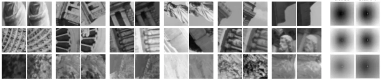
a data-driven approach should learn a more meaningful and distinct representation of image patches, while being invariant to changes in lighting and viewpoint conditions. This is in contrast with the hand-crafted approach, in which datasets play a less-direct role. A good example of data-driven approaches is in Brown et al. (2011), where they made a patches dataset using the 3D reconstruction of the Statue of Liberty (New York), Notre Dame (Paris), and Half Dome (Yosemite) from the photos and the multi-view stereo data of Snavely et al.

(2008);Goesele et al. (2007). This dataset, now known as Multi-View Stereo (MVS) dataset, is composed of a large set of 64x64 patches, mostly depicting buildings.

Consequently, a descriptor train with such a dataset will be biased toward buildings and may very well fail on other datasets, such as a household objects dataset, to name one. Nevertheless,

Brown et al.(2011) showed with their dataset that learning a parametric function on one of the three buildings and testing on another one, made their descriptor offer a better performance than a generic one such as SIFT. Despite the bias induced by the dataset, learned descriptors can thus be useful as long as the data used to train them is appropriately selected for the task. With encouraging results of machine learning approaches such as Brown et al. (2011), it was expected to see a deep learning approach such asSimo-Serra et al.(2015);Paulin et al.(2015) apply CNN to the local feature descriptor task. In the case of Paulin et al. (2015), they ap-proximate a kernel map in an unsupervised way using the Convolution Kernel Network (CKN) from Mairal et al. (2014) that was developed to be more simple, easy to train and invariant than normal CNN. Then, their network takes image patches as input and produced kernel map approximations, which serve as the descriptions. To train this descriptor, they prepared a new patches dataset using landmark images of Rome taken from Li et al. (2010). They tested their approach on the unseen part of their Rome dataset, as well as other benchmarks, and showed on par or better performance than supervised CNN.