HAL Id: tel-01243340
https://pastel.archives-ouvertes.fr/tel-01243340v2
Submitted on 25 Apr 2016HAL is a multi-disciplinary open access archive for the deposit and dissemination of sci-entific research documents, whether they are pub-lished or not. The documents may come from teaching and research institutions in France or abroad, or from public or private research centers.
L’archive ouverte pluridisciplinaire HAL, est destinée au dépôt et à la diffusion de documents scientifiques de niveau recherche, publiés ou non, émanant des établissements d’enseignement et de recherche français ou étrangers, des laboratoires publics ou privés.
Image Databases
Jan Margeta
To cite this version:
Jan Margeta. Machine Learning for Simplifying the Use of Cardiac Image Databases. Signal and Image Processing. Ecole Nationale Supérieure des Mines de Paris, 2015. English. �NNT : 2015ENMP0055�. �tel-01243340v2�
N°: 2009 ENAM XXXX
MINES ParisTech
Centre de Mathématiques Appliquées
Rue Claude Daunesse B.P. 207, 06904 Sophia Antipolis Cedex, France
École doctorale n° 84 :
Sciences et technologies de l’information et de la communication
présentée et soutenue publiquement par
Ján MARGETA
le 14 Décembre 2015
Apprentissage automatique pour simplifier
l’utilisation de banques d’images cardiaques
Machine Learning for Simplifying
the Use of Cardiac Image Databases
Doctorat ParisTech
T H È S E
pour obtenir le grade de docteur délivré par
l’École nationale supérieure des mines de Paris
Spécialité “ Contrôle, optimisation et prospective ”
Directeurs de thèse : Nicholas AYACHE et Antonio CRIMINISI
T
H
È
S
E
JuryM. Patrick CLARYSSE, DR, Creatis, CNRS, INSA Lyon Rapporteur
M. Bjoern MENZE, Professeur, ImageBioComp Group, TU München Rapporteur
M. Hervé DELINGETTE, DR, Asclepios Research Project, Inria Sophia Antipolis Président
M. Antonio CRIMINISI, Chercheur principal, MLP Group, Microsoft Research Cambridge Examinateur
M. Hervé LOMBAERT, Docteur, Asclepios Research Project, Inria Sophia Antipolis Examinateur
M. Alistair A. YOUNG, Professeur, Auckland Bioengineeding Institute, University of Auckland Examinateur
Acknowledgments
This has been an incredible journey. A journey of learning and self-discovery. Many people, papers, or books have helped to shape the thesis and my thinking. I have been lucky to have had amazing mentors and have worked with many incredibly smart people. A complete list would easily take up another chapter. It has been a great pleasure and honour to work and spend time with you. Thank you all!
First, I would like to thank my PhD supervisors and mentors. I fell many times but they never gave up on me, always helped me to stand back up and to pull myself forward. To Nicholas Ayache, not only for inviting me to join Asclepios, but also for sharing his vision with me and for his inspiring leadership of our vibrant team. Thank you for helping me to get better clarity in cloudy times. I am also immensely grateful to Antonio Criminisi. For his encouragement, for the discussions that helped to spark new ideas. For showing me how to practically do machine learning and the importance of visualisation. I am also indebted to you for the opportunity to visit MSR in Cambridge and spend a fantastic summer on a fascinating project.
I am grateful to Hervé Lombaert for his enthusiasm that never vaned, for thor-oughly rereading the thesis and helping me to find the right voice. For all the unforgettable moments at and outside of Asclepios. I would like to express my gratitude to Peter Kontschieder, my MSR summer mentor, for sharing his endless passion and energy, for pushing me into challenging problems and for helping me to improve my focus and iteration speed. I would like to thank to all permanent re-searchers at Asclepios. To Maxime Sermesant, for all cardiac discussions, to Hervé Delingette for inspiring work and presiding my jury, to Xavier Pennec for inspiring scientific rigor, to Olivier Clatz for sharing his enterpreneurial spirit with me.
I would like to thank to all of my jury members and my thesis reviewers for joining us in Sophia Antipolis from faraway lands, for thoroughly reading the thesis and for sharing their feedback with me. I enjoyed the pre-defence chat with Patrick Clarysse, thank you for the encouraging words. I am grateful to Bjoern Menze, for the discussions we have had during his visits to Asclepios. They helped me better understand what content retrieval should be about. I cannot thank enough to Alistair Young. Not only for providing us with the fantastic data resource but also for making the world of cardiac imaging a better place. For the care put into the Cardiac atlas project and for the number of inspiring papers that influenced my work. My big thanks and kudos go to Catalina Tobon and Avan Suinesiaputra, for making science more objective and for organising two incredibly fun challenges that I had the chance to participate in.
I am grateful to all cardiologists I have met and had the chance to work with. In particular, my thanks go to Daniel C Lee, for input on our papers, I learned a lot from your feedback. To Philipp Beerbaum for talking us through real MRI acquisitions at St. Thomas Hospital, and for patiently responding to a number of naive cardiac questions. To Andrew Taylor and the whole GOSH team. I truly
enjoyed the exchanges we have had. They helped me to get better understanding of the clinical challenges.
This would be so much more difficult without the flawless support of Isabelle Strobant. I would also like to thank Scarlet Schwiderski-Grosche and Laurent Mas-soulié for making the joint PhD with MSR possible. I am grateful to Valérie Roy, for her incredible help in the final and most important stage of the thesis. To Vi-bot, the finest master in computer vision, for the foundations it gave me. To Prof. Hamed Sari-Sarraf for an impeccable machine learning course.
I have had the chance to share the office with some truly remarkable people. Thank you all for your friendships and for the good times we have had. To Stéphanie and Loïc, for their kindness and patience with many of my questions. To Thomas for his wit, cheerfulness and for always being there. To Clair for his curiosity. To Darko for your inspiring healthier research lifestyle. Thanks to all PhDs, Post-Docs and engineers at Asclepios. For providing the foundation for all that is so great about the team. My huge thanks go to Chloé, Krissy (also for being a fantastic scientific wife), Marine, Rocío, and Flo for the great times together in and out of the lab in the nature. To Ezequiel, for helping me out with my first academic paper. To Matthieu, Raphael, Sophie, Marc-Michel, for selflessly being there till the last rehearsal. To Nicolas and Vikash, for sharing laughs and the path till the end of the Mesozoic era. To Adityo, Alan, Barbara, Bishesh, Christof, Federico, Hakim, Héloïse, Hugo, Irina, John, Loïc, Marco, Marzieh, Mehdi, Michael and Roch. I had an incredible summer internship at MSR in Cambridge. I am grateful to Yani and Sam for the “deep talks” and crawls “under the table”, to Qinxun for great time and culinary experiences (keep rolling Jerry!), Ina, Diana and Jonas. To Rubén and Oscar.
To my friends, to Kos and Amanda, Natalka and Zhanwu, Alex, Beto, Emka, Tjaša and Xtian for their undisputed friendship. To Math, Issis, Hernán and Arjan for the wonderful time during my visits of Paris, Barcelona and London. To Zoom, Nico, Clém, Francis for their hospitality. To my kayak friends, for their camaraderie, and for keeping me physically alive and mentally sane. To Oli for showing me another perspective on the world. To Raph, Laurent, Hervé, Thierry, Fred, Eric and the whole SPCOCCK. To Steffi and Pascal. I am indebted to Mumu and the teams at CHU Nice and Bratislava for saving my life.
Last, but not least, none of this would be possible without the love and support of my family, I am deeply grateful for always believing in me. To my dad, a tremendous source of inspiration to me, to my mum for constantly pushing me till the finish line, and to Karol, the best brother ever! To Magdalénka, my (not only) tireless copywriter, for her endless love and patience along this journey.
This work was supported by Microsoft Research through its PhD Scholarship Programme and ERC Advanced Grant MedYMA 2011-291080. The research leading to these results has received funding from the European Union’s Seventh Framework Programme for research, technological development and demonstration under grant agreement no. 611823 (VP2HF).
Table of Contents
1 Introduction 5
1.1 The dawn of the cardiac data age . . . 5
1.2 Challenges of large cardiac data organisation . . . 6
1.2.1 Data aggregation from multi-centre studies . . . 6
1.2.2 Data standardisation . . . 7
1.2.3 Retrieving similar cases . . . 8
1.2.4 Data annotation and consensus . . . 8
1.2.5 The need for automated tools . . . 8
1.3 A deceptively simple problem . . . 9
1.3.1 Automating the task . . . 10
1.3.2 The machine learning approach . . . 10
1.4 Research questions of this thesis . . . 11
1.4.1 Automatic clean-up of missing DICOM information . . . 11
1.4.2 Segmentation of cardiac structures . . . 12
1.4.3 Crowdsourcing cardiac attributes . . . 12
1.4.4 Cardiac image retrieval . . . 12
1.5 Manuscript organisation . . . 13
1.6 List of publications . . . 13
2 Learning how to recognise cardiac acquisition planes 17 2.1 Brief introduction to cardiac data munging . . . 18
2.2 Cardiac acquisition planes . . . 19
2.2.1 The need for automatic plane recognition . . . 19
2.2.2 Short axis acquisition planes . . . 20
2.2.3 Left ventricular long axis acquisition planes . . . 20
2.3 Methods . . . 22
2.3.1 Previous work. . . 22
2.3.2 Overview of our methods . . . 22
2.4 Using DICOM orientation tag . . . 23
2.4.1 From DICOM metadata towards image content . . . 24
2.5 View recognition from image miniatures . . . 24
2.5.1 Decision forest classifier . . . 24
2.5.2 Alignment of radiological images . . . 26
2.5.3 Pooled image miniatures as features . . . 26
2.5.4 Augmenting the dataset with geometric jittering . . . 28
2.5.5 Forest parameter selection . . . 28
2.6 Convolutional neural networks for view recognition . . . 29
2.6.1 Layers of the Convolutional Neural networks . . . 30
2.6.3 Network architecture . . . 33
2.6.4 Reusing Convolutional neural network (CNN) features tuned for visual recognition . . . 34
2.6.5 CardioViewNet architecture and parameter fine-tuning. . . . 35
2.6.6 Training the network from scratch . . . 36
2.7 Validation . . . 37
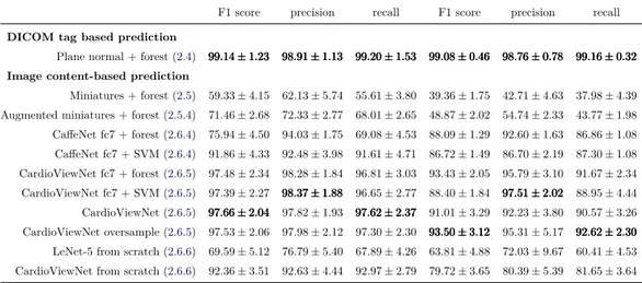
2.8 Results and discussion . . . 38
2.9 Conclusion and perspectives . . . 42
3 Segmenting cardiac images with classification forests 43 3.1 Segmentation of the left ventricle . . . 44
3.1.1 Measurements in cardiac magnetic resonance imaging . . . . 44
3.1.2 Previous work. . . 45
3.1.3 Overview of our method . . . 46
3.1.4 Layered spatio-temporal decision forests . . . 47
3.1.5 Features for left ventricle segmentation. . . 48
3.1.6 First layer: Intensity and pose normalisation . . . 51
3.1.7 Second layer: Learning to segment with the shape . . . 54
3.1.8 Validation . . . 55
3.1.9 Results and discussion . . . 56
3.1.10 Volumetric measure calculation . . . 58
3.1.11 Conclusions . . . 58
3.2 Left atrium segmentation . . . 59
3.2.1 Dataset . . . 60
3.2.2 Preprocessing . . . 60
3.2.3 Training forests with boundary voxels . . . 60
3.2.4 Segmentation phase . . . 60
3.2.5 Additional channels for left atrial segmentation . . . 60
3.2.6 Validation . . . 62
3.2.7 Results and discussion . . . 64
3.2.8 Conclusions . . . 64
3.3 Conclusions and perspectives . . . 65
3.3.1 Perspectives. . . 65
4 Crowdsourcing semantic cardiac attributes 67 4.1 Describing cardiac images . . . 68
4.1.1 Non-semantic description of the hearts . . . 68
4.1.2 Semantic attributes . . . 69
4.2 Attributes for failing post-myocardial infarction hearts . . . 70
4.2.1 Pairwise comparisons for image annotation . . . 72
4.2.2 Selected attributes for shape, motion and appearance . . . . 73
4.3 Crowdsourcing in medical imaging . . . 74
4.3.1 A ground-truth collection web application . . . 74
Table of Contents v
4.5 Spectral description of cardiac shapes . . . 77
4.6 Texture features to describe image quality . . . 78
4.7 Evaluation and results . . . 78
4.7.1 Data and preprocessing . . . 78
4.7.2 Evaluation . . . 79
4.8 Conclusions and perspectives . . . 79
4.8.1 Perspectives . . . 80
5 Learning how to retrieve semantically similar hearts 83 5.1 Content based retrieval in medical imaging . . . 84
5.1.1 Visual information search behaviour in clinical practice . . . 84
5.1.2 Where are we now? . . . 85
5.2 Similarity for content-based retrieval . . . 86
5.2.1 Bag of visual words histogram similarity . . . 86
5.2.2 Segmentation-based similarity. . . 86
5.2.3 Shape-based similarity . . . 87
5.2.4 Registration-based similarity . . . 87
5.2.5 Euclidean distance between images . . . 87
5.2.6 Using decision forests to approximate image similarity . . . . 88
5.3 Neighbourhood approximating forests . . . 89
5.3.1 Learning how to structure the dataset . . . 90
5.3.2 Finding similar images . . . 90
5.3.3 NAFs for post-myocardial infarction hearts . . . 91
5.4 Learning the functional similarity . . . 91
5.4.1 Cluster compactness based on ejection fraction difference . . 91
5.4.2 Preprocessing . . . 91
5.4.3 Spatio-temporal image features . . . 95
5.5 Validation and results . . . 98
5.5.1 Retrieval experiment . . . 98
5.5.2 Feature importance. . . 99
5.6 Discussion and perspectives . . . 104
5.6.1 Limitations . . . 105
5.6.2 Perspectives . . . 105
6 Conclusions and perspectives 107 6.1 Summary of the contributions . . . 107
6.1.1 Estimating missing metadata from image content . . . 107
6.1.2 Segmentation of cardiac images . . . 108
6.1.3 Collection of ground-truth for describing the hearts with se-mantic attributes . . . 109
6.1.4 Structuring the datasets with clinical similarity . . . 110
6.2 Perspectives . . . 111
6.2.1 Multimodal approaches . . . 111
6.2.3 Generating more data . . . 112
6.2.4 Data augmentation. . . 112
6.2.5 Collecting labels through crowdsourcing and gamification . . 113
6.2.6 Moving from diagnosis to prognosis. . . 113
A Distance approximating forests for sparse label propagation 115 A.1 Introduction. . . 115
A.2 Previous work . . . 116
A.3 Distance approximating forests . . . 117
A.3.1 Finding shortest paths to the labels . . . 118
A.4 Results and discussion . . . 120
A.4.1 Synthetic classification example . . . 120
A.4.2 Towards interactive cardiac segmentation . . . 121
A.5 Conclusions . . . 123
A.5.1 Perspectives. . . 123
B Regressing cardiac landmarks from CNN features for image align-ment 125 B.1 Introduction. . . 125
B.2 Aligning with landmarks and regions of interest . . . 126
B.3 Definition of cardiac landmarks . . . 126
B.4 Cascaded shape regression . . . 128
B.5 Conclusions . . . 131
C A note on pericardial effusion for retrieval 133 C.1 Overview . . . 133
C.2 Introduction. . . 133
C.3 Pericardial effusion based similarity. . . 134
C.3.1 Compactness on effusion. . . 134
C.4 An additional image channel . . . 134
C.5 Retrieving similar images . . . 135
C.6 Conclusions and perspectives . . . 135
D Abstracts from coauthored work 137 E Sommaire en français 141 E.1 L’aube du Big Data cardiaque. . . 141
E.2 Les défis pour l’organisation des données cardiaques à grande échelle 142 E.2.1 Agrégation des données provenant des études multi-centriques142 E.2.2 Normalisation des données. . . 142
E.2.3 Récupération des cas similaires . . . 143
E.2.4 Annotation des données et le consensus . . . 143
E.2.5 Le besoin d’outils automatisés . . . 144
E.3 Un problème trompeusement simple . . . 144
Table of Contents vii
E.3.2 L’approche de l’apprentissage automatique . . . 145
E.4 Les questions de recherche de cette thèse. . . 146
E.4.1 Nettoyage automatique des balises DICOM . . . 146
E.4.2 Segmentation des structures cardiaques . . . 146
E.4.3 Approvisionnement par la foule et description sémantique . . 147
E.4.4 Peut-on récupérer automatiquement les coeurs semblables ? . 147 E.5 Organisation du manuscrit. . . 148
E.6 Sommaires des chapitres . . . 148
E.6.1 Reconnaisance des plans d’acquisition cardiaques . . . 148
E.6.2 Segmentation d’images cardiaques . . . 149
E.6.3 Approvisionnement par la foule des attributs semantiques . . 150
E.6.4 Recherche d’image par le contenu. . . 150
E.7 Conclusions et perspectives . . . 151
E.7.1 Synthèse des contributions. . . 151
E.7.2 Perspectives . . . 155
Abbreviations and Acronyms
AHA American Heart Association
Ao aorta
AoD descending aorta AV aortic valve BOW Bag of words
CAP Cardiac atlas project
CBIR Content based image retrieval CMR Cardiac magnetic resonance imaging CNN Convolutional neural network CT Computed tomography DE-MRI Delayed enhancement MRI DF Decision forest
DICOM Digital Imaging and Communications in Medicine
DTW Dynamic time warping ECG Electrocardiogram ED end diastole
EDV end diastolic volume EF ejection fraction
EHR Electronic health record ES end systole
ESV end systolic volume GPU Graphical processing unit GRE Gradient echo
HIPAA Health Insurance Portability and Accountabil-ity Act
LA left atrium
LoG Laplacian of Gaussian LRN Local response normalisation LV left ventricle
LVC left ventricular cavity
LVOT Left ventricular outflow tract ML machine learning
MR Magnetic resonance
MRI Magnetic resonance imaging MV mitral valve
NAF Neighbourhood approximating forest NPV Negative predictive value
PACS Picture archiving and communication system PCA Principal Component Analysis
PET Positron emission tomography PM papillary muscle
PPM posterior papillary muscle PPV Positive predictive value RA right atrium
ReLU Rectified linear unit RGB Red-Green-Blue RV right ventricle SAX short axis
SCMR Society for Cardiac Magnetic Resonance SGD Stochastic gradient descent
Abbreviations and Acronyms 3
SNOMED CT Systematized Nomenclature of Medicine -Clinical Terms
SSFP Steady state free precession
STACOM Statistical Atlases and Computational Model-ing of the Heart
SVM Support vector machine TOF Tetralogy of Fallot
TV tricuspid valve
Chapter 1
Introduction
Contents
1.1 The dawn of the cardiac data age. . . . 5
1.2 Challenges of large cardiac data organisation. . . . 6
1.2.1 Data aggregation from multi-centre studies . . . 6
1.2.2 Data standardisation. . . 7
1.2.3 Retrieving similar cases . . . 8
1.2.4 Data annotation and consensus . . . 8
1.2.5 The need for automated tools . . . 8
1.3 A deceptively simple problem . . . . 9
1.3.1 Automating the task . . . 10
1.3.2 The machine learning approach . . . 10
1.4 Research questions of this thesis . . . . 11
1.4.1 Automatic clean-up of missing DICOM information . . . 11
1.4.2 Segmentation of cardiac structures . . . 12
1.4.3 Crowdsourcing cardiac attributes . . . 12
1.4.4 Cardiac image retrieval . . . 12
1.5 Manuscript organisation . . . . 13
1.6 List of publications . . . . 13
1.1
The dawn of the cardiac data age
The developments in cardiology over the last century (Cooley and Frazier, 2000;
Braunwald, 2014) have been quite spectacular. Many revolutions have happened since the first practical Electrocardiogram (ECG) by Einthoven in 1903. These include cardiac catheterization (1929), heart and lung machine and first animal models in the 1950s, minimally invasive surgeries (1958), and drug development (β blockers (1962), statins (1971), and angiotensins (1974)). The diagnostic imaging of the heart has also vastly improved. The post-war development of cardiac Ultrasound (US), Computed tomography (CT) (1970s) and Magnetic resonance imaging (MRI) (1980s) have helped us to non-invasively peek into the heart at a remarkable level of detail.
All of these advances have dramatically changed the course of cardiovascular disease management and by 1970 the mortality due to these diseases in high income countries has tipped and has been steadily declining (Fuster and Kelly,2010, p52) ever since. Yet, the cardiovascular diseases remain the number one killer in the world (Nichols et al., 2012, p 10;Roger et al.,2011), causing 47% of all deaths in
Europe.
We are at the dawn of the age where new cardiac image acquisition techniques, predictive in silico cardiac models (Lamata et al.,2014), realistic image simulations (Glatard et al., 2013;Prakosa et al., 2013; Alessandrini et al., 2015), real-time pa-tient monitoring (Xia et al.,2013), and large-scale cardiac databases (Suinesiaputra et al.,2014a;Petersen et al.,2013;Bruder et al.,2013) become ubiquitous and have the chance to further improve cardiac health and our understanding.
Data within these databases are only as useful as the questions they can help to answer, the insights they can generate, and the decisions they enable to make. Large population clinical studies with treatment recommendations can be made, supporting evidence can be tailored for each patient individually. Treatment can be adjusted by looking at similar, previously treated patients, comparing their out-comes, and predicting what is likely to happen. New teaching tools can be developed using the data to create virtual patient case studies and surgery simulations on 3D-printed models (Bloice et al.,2013;Kim et al.,2008;Jacobs et al.,2008) and boost the education and practice of cardiologists.
1.2
Challenges of large cardiac data organisation
The opportunities for novel uses of large image databases are countless, however, the usage of these databases poses new challenges. Rich cardiac collections with relevant images (including many rare conditions) are scattered across thousands of Picture archiving and communication system (PACS) servers across many countries and hospitals. Data coming from these heterogeneous sources are not only massive, but often also quite unstructured and noisy.
1.2.1 Data aggregation from multi-centre studies
The biobanks and international consortia managing medical imaging databases, such as the UK biobank (Petersen et al.,2013), the Cardiac atlas project (CAP) ( Fon-seca et al.,2011) or the VISCERAL project (Langs et al.,2013), have solved many difficult problems in ethics of data sharing, medical image organisation and data dis-tribution — in particular, when aggregating the data from multiple sources. The PACS together with the Digital Imaging and Communications in Medicine (DI-COM) standards have been invaluable in these efforts. Studies coming from multiple centres often use specific nomenclature, follow different guidelines or utilise different acquisition protocols. In these cases, even these standards are not sufficient.
1.2. Challenges of large cardiac data organisation 7
1.2.2 Data standardisation
The image collections on PACS servers can be queried by patient information (e.g. ID, name, birth date, sex, height, weight), image modality, study date and other DICOM tags, sometimes by study description, custom tags of the clinicians, associ-ated measurements (e.g. arterial blood pressure and cardiac heart rate) and disease or procedure codes. See Fig. 1.1for an example of such interface.
Figure 1.1: Cardiac atlas project web client interface.
There is no standard way to store some of the important image related infor-mation (e.g. the cardiac acquisition image plane inforinfor-mation), where the naming depends on custom set-up of the viewing workstation and on the language prac-ticed at the imaging centre. Even the standard DICOM tags often contain vendor specific nomenclature. For example, the same Cardiac magnetic resonance imaging (CMR) acquisition sequences are branded differently across the Magnetic resonance (MR) machine vendors (Siemens,2010). While some implementation differences ex-ist, these are not relevant for image interpretation, and the terminology could be significantly simplified (Friedrich et al.,2014). Parsing electronic publications with images is even a bigger challenge. These images are rarely in DICOM format and only the image content with textual description is available.
Such differences reduce our ability to effectively query and explore the databases for relevant images. The standardisation can be enforced by strictly following guide-lines during image acquisition, and consistently using terminologies to encode the associated information such as the Systematized Nomenclature of Medicine - Clini-cal Terms (SNOMED CT) (Stearns et al.,2001). Care has to be taken to eliminate manual input errors. Images previously stored in the databases without the stan-dardised information should be revisited for better accessibility.
1.2.3 Retrieving similar cases
Manually crawling through these growing databases to find similar previously treated patients (with supporting evidence) becomes very time consuming. Delivering archived images from PACS is, in practice, quite slow for such exploratory use. In addition, the cardiac imaging data stored in the databases are frequently 3D+t sequences, and important details can be easily missed during such visual inspection.
An alternative to this brute-force approach is to consistently describe the images with more compact representations. This prepares the cardiac image databases for future image retrieval. Though, it limits the search to the annotated data or to the cases known to the particular clinician. Most of the unannotated data therefore never gets used again and unused data means useless data.
1.2.4 Data annotation and consensus
Annotating these images simplifies their later reuse. However, together with the growth of the data, the demand for manual input becomes an increasing burden on the expert raters. One way to tackle this is to reduce the annotation task into very simpler questions that can be answered by a larger number of less experienced raters, for example via crowdsourcing.
As studied bySuinesiaputra et al.(2015), the variability of different radiologists (experts following the same guidelines) is not negligible. For example, in left ven-tricle (LV) segmentation, the papillary muscles (PMs) are myocardial tissue and therefore according to Schulz-Menger et al. (2013) should ideally be included in the myocardial mass and excluded from the left ventricular cavity (LVC) volume calculation. The corresponding reference values for volumes and masses (Maceira et al.,2006;Hudsmith†et al.,2005) should be used in this case. Some tools include the papillary muscles into the cavity volume instead. In this case a different set of reference values should be considered (Natori et al., 2006). The two reported measures can differ substantially. Ultimately, the PMs are part of the disease pro-cess (Harrigan et al.,2008) and deserve individual attention on their own.
The acquisition centres are equipped with different software tools and not all of these tools are equally capable. We still have a long way ahead to achieve reproducible extraction of image-based measures and consistent description of all relevant image information, especially given the constantly evolving guidelines.
1.2.5 The need for automated tools
For success in large scale analysis and use of the data, efficient ways of automatic clean-up and description of the cardiac data coming from several clinical centres with tools scalable to large data (Medrano-Gracia et al.,2015) are primordial. As we will see on the following example, manual design of such tools can rapidly become quite challenging.
1.3. A deceptively simple problem 9
1.3
A deceptively simple problem
Examine the following four CMR mid-ventricular short axis (SAX) slices obtained using the Steady state free precession (SSFP) acquisition sequence shown inFig. 1.2. They belong to four individuals with different pathologies. One of them is an image of a healthy heart, another belongs to a patient after a myocardial infarction in the lateral wall, the third to a patient with a severely failing and non-compacting left ventricle and the last one shows a patient with idiopathic pericardial effusion. Can you correctly tell which one is which?
Figure 1.2: Four cardiac pathologies on MRI: heart with pericardial effusion, post lateral wall myocardial infarction heart, left ventricular non-compaction and a healthy heart. Can you identify them?1
This task of pathology identification is seemingly effortless for a person expe-rienced in interpretation of cardiac images. Intuitively, we could recognise the post-myocardial infarction heart by a marked thinning of the lateral wall due to a transmural infarction and subsequent myocardial necrosis. One might also note sternal wire artefacts from a prior surgery. The failing non-compacting heart
man-ifests itself with massive dilation, prominent trabeculations in the left ventricular cavity, and significant reduction in myocardial contractility (best seen on cinematic image sequences). The pericardial effusion can be seen as a bright ring of liquid outside of the myocardium and swinging heart motion. And finally, the healthy heart looks “normal.”
1.3.1 Automating the task
Only when we try to write a program to mimic this reasoning on a computer we can start to fully appreciate the true complexity of the visual tasks performed by the brain. The simplicity of relevant information extraction from the images is very deceptive. Intuitive concepts like the myocardial thinning, the cavity dilation, low contractility, bright ring, or swinging motion are concepts unknown to a machine. Not to mention the more global problem to automatically tell that all these images are short axis slices coming from a SSFP MR acquisition sequence.
One of the possibilities to extract this information by a computer is to start writing a set of rules. Myocardial thinning measurement can be measured as the length of the shortest line across the myocardium, counting pixels between two edges separating the white blob (the blood pool) and the grey (except for the effusion case) outer surroundings of the heart. Dilation is linked to the number of voxels within the ventricular blood pool and the cavity diameter. Both of these measures can be computed from segmentation of the left ventricular myocardium. The contractility can be estimated from displacement of the pixels, e.g., via image registration. The subtle changes we might want to recognise are easily overshadowed by acquisition differences, e.g., images coming from different MR acquisition machines, acquisition artefacts or differences in image orientation and heart position in the images. The images have no longer similar resolutions and image quality, tissue intensities on CMR between different machines do not match, acquisition artefacts are present or vendor specific variations of similar acquisition protocols are used. We soon discover that the set of rules to encode the relevant information and extract features to describe the cardiac images is endless.
1.3.2 The machine learning approach
The machine learning approach is quite different. Instead of manually hardcoding the rules, we specify a learning model and let the learning algorithm automatically figure out a set of rules by looking at the data, i.e., to train the model. In the supervised learning setting, a set of examples together with desired outputs (e.g. images and their voxel-wise segmentations) is shown the training algorithm. The algorithm then picks rules that best map the inputs to the desired outputs. It is important that the learnt model generalises, i.e., can reliably predict outputs for previously unseen images while ignoring irrelevant acquisition differences.
1Top left: Lateral infarction with thinning, top right: healthy, bottom left: left ventricular
1.4. Research questions of this thesis 11
Although good prediction is desirable, it is common to use “less than perfect” machine learning systems in a loop, and improve the models over time, when more data arrives. Also when guidelines change, these algorithms can be retrained and the images can be reparsed. Incorrect predictions can be fixed and added to the new training set and the model can then be retrained.
Machine learning in medical imaging has become remarkably important. This is partly due to the algorithmic improvements but mainly thanks to the increased availability of large quantities of data. While there are many machine learning algorithms, there is not (yet) a perfect one dealing with all the tasks at hand. One that is working for both large and small datasets.
Throughout this thesis we will use mainly three families of supervised machine learning (ML) algorithms: Linear regression models (the Support vector machines (SVMs) (Cortes and Vapnik,1995) and ridge regression (Golub et al., 1979)), the Decision forests (DFs) (Ho,1995;Amit and Geman,1997;Breiman,1999), and the Convolutional neural network (CNN) (Fukushima,1980;LeCun et al.,1989).
1.4
Research questions of this thesis
This thesis aims to answer the following global question: “How can we simplify the use of CMR image databases for cardiologists and researchers using machine learning?” To help us answer this question, we addressed some of the main challenges introduced in Section 1.2.
1.4.1 How can we clean up and standardise DICOM tags for easier
filtering and grouping of image series?
One of the first problems we face in cardiac imaging when dealing with large multi-vendor databases is the lack of standardisation in used notation in acquisition pro-tocols (Friedrich et al., 2014) or naming of cardiac acquisition planes. Especially the knowledge of cardiac planes is essential for grouping the images into series and choosing the right image processing pipeline.
Chapter 2 presents our two methods for fixing noisy DICOM metadata with
information estimated directly from image content. Our first method to recognise CMR acquisition planes uses classification forests applied on image miniatures. We show how cheaply generated new images can help to improve the recognition.
We then show how we modify a state of the art technique in a large scale visual object recognition, based on CNNs, to a much smaller cardiac imaging dataset. Our second method recognises short axis and 2-, 3- and 4-chamber long axis views with very promising recognition performance.
InAppendix Bwe show how the CNN-based features can be reused to regress
1.4.2 Can we teach the computer to understand cardiac anatomy and to segment cardiac structures from MR images?
Once we can describe cardiac images based on their views and merge them into spatio-temporal 3D+t series we can move on to teach the computer the basics of cardiac anatomy, i.e., how to segment the cardiac images. Successful segmentation is essential to index cardiac images based on standard volumetric measures such as systolic and diastolic volume, ejection fraction, and myocardial mass.
In Chapter 3 we extend the previous work on semantic segmentation using
classification forests (Shotton et al.,2008;Geremia et al.,2011). We show how our modified algorithm learns to segment left ventricles from 3D+t MR short axis SSFP sequences without imposing any shape prior. Our decision forest classifier is trained in a layered fashion, and we propose new spatio-temporal features to classify the 3D+t sequences. We show that avoiding to hard-code the segmentation problem helps us to easily adapt this technique to segment other cardiac structures, the left atria — the black box of the heart, both from CMR and CT. We contributed these algorithms to two comparison studies for fair evaluation.
InAppendix Awe propose a segmentation method exploiting unlabelled data
in a semi-supervised setting to learn how to segment from sparse annotations.
1.4.3 How can we collect data needed by the computer for training
of the machine learning algorithms and learn how to describe the hearts with semantically meaningful attributes?
Most of the practical machine learning problems are currently still solved in a fully supervised manner. It is therefore essential to acquire the ground-truth. Chapter 4
deals with label collection for machine learning algorithms. We design a web-based tool for crowd-sourcing of cardiac attributes and use it to collect pairwise image annotations. We describe the cardiac shapes with their spectral signatures and use a linear predictor based on SVM classifier to learn ordering of the images based on their attribute values. Our preliminary results suggest that in addition to volumetric measurements obtainable from cardiac segmentations, the hearts could be described by cardiac attributes.
1.4.4 Can we automatically retrieve similar hearts?
The image similarity depends on the clinical question to be answered. Queries we might want to ask the retrieval system can be quite variable. Chapter 5 builds
on the Neighbourhood approximating forest (NAF) of Konukoglu et al.(2013) and presents our pipeline to learn shape, appearance and motion similarities between car-diac images and how we use them to structure the spatio-temporal carcar-diac datasets. We show how hearts with similar properties (similar ejection fraction) can be ex-tracted from the database. In (Bleton et al.,2015), we then used a similar technique to localise cardiac infarcts from dynamic shapes only (no contrast agent needed).
1.5. Manuscript organisation 13
1.5
Manuscript organisation
The presented thesis is organised around our published work and our work in prepa-ration for submission. The manuscript also roughly progresses from global towards fine-grained description of the cardiac images. Each chapter in this thesis attempts to answer one of the objectives and to bring content-based retrieval of images from large-scale CMR databases closer to reality.
First, we train a system to fix image tags that are not captured by DICOM directly from image content. InChapter 2, we show how to automatically recognise cardiac planes of acquisition. In Chapter 3, we propose a flexible automatic seg-mentation technique that learns to segment cardiac structures from spatio-temporal image data, using simple voxel-wise ground-truth as input, that could be used for automatic measurements. InChapter 4, we suggest a way of collecting annotations necessary for training of automatic algorithms, and to describe the cardiac images with sets of semantic attributes. Finally, in Chapter 5, we propose an algorithm to structure the datasets and find similar cases with respect to different clinical criteria.
Chapter 6concludes the thesis with perspectives and future work. In the appendices, we illustrate how unlabelled data can be used for guided image segmentation ( Ap-pendix A), how to estimate cardiac landmarks for image alignment (Appendix B), or how to enhance pericardial effusion for image retrieval (Appendix C).
1.6
List of publications
Journal articles• J. Margeta, A. Criminisi, R. Cabrera Lozoya, D. C. Lee, and N. Ayache,
“Fine-tuned convolutional neural nets for cardiac MRI acquisition plane recog-nition”, Computer methods in biomechanics and biomedical engineering:
Imag-ing & visualisation, 2015.
• C. Tobon-Gomez, A. Geers, J. Peters, J. Weese, K. Pinto, R. Karim, M. Ammar, A. Daoudi, J. Margeta, Z. Sandoval, B. Stender, Y. Zheng, M. A. Zuluaga, J. Betancur, N. Ayache, M. A. Chikh, J.-L. Dillenseger, M. Kelm, S. Mahmoudi, S. Ourselin, A. Schlaefer, T. Schaeffter, R. Razavi, and K. Rhode,
“Benchmark for Algorithms Segmenting the Left Atrium From 3D CT and MRI Datasets”, IEEE Transactions on Medical Imaging, vol. 34, no. 7, pages
1460 1473, 2015.
• A. Suinesiaputra, B. R. Cowan, A. O. Al-Agamy, M. A. Elattar, N. Ayache, A. S. Fahmy, A. M. Khalifa, P. Medrano-Gracia, M. P. Jolly, A. H. Kadish, D. C. Lee, J. Margeta, S. K. Warfield, and A. A. Young, “A collaborative resource
to build consensus for automated left ventricular segmentation of cardiac MR images”, Medical Image Analysis, vol. 18, no. 1, pages 50 62, 2014.
Peer reviewed conference and workshop papers
• J. Margeta, A. Criminisi, D. C. Lee, and N. Ayache, “Recognizing cardiac
magnetic resonance acquisition planes”, in Conference on Medical Image
Un-derstanding and Analysis (MIUA 2014), 2014. Oral podium presentation. • J. Margeta, K. S. McLeod, A. Criminisi, and N. Ayache, “Decision forests
for segmentation of the left atrium from 3D MRI”, in International
Work-shop on Statistical Atlases and Computational Models of the Heart. Imaging and Modelling Challenges, Held in conjunction with MICCAI 2013, Beijing, Lecture Notes in Computer Science, vol. 8830, pages 49 56, O. Camara, T. Mansi, M. Pop, K. Rhode, M. Sermesant, and A. Young, Eds., Springer Berlin / Heidelberg, 2014. Oral podium presentation.
• J. Margeta, E. Geremia, A. Criminisi, and N. Ayache, “Layered
Spatio-temporal Forests for Left Ventricle Segmentation from 4D Cardiac MRI Data”,
in International Workshop on Statistical Atlases and Computational Models of the Heart. Imaging and Modelling Challenges, Held in conjunction with MICCAI 2011, Toronto, Lecture Notes in Computer Science, vol. 7085, pages 109 119, O. Camara, E. Konukoglu, M. Pop, K. Rhode, M. Sermesant, and A. Young, Eds., Springer Berlin / Heidelberg, 2012, Oral podium presentation. • H. Bleton, J. Margeta, H. Lombaert, H. Delingette, and N. Ayache,
“My-ocardial Infarct Localisation using Neighbourhood Approximation Forests”, in
International Workshop on Statistical Atlases and Computational Models of the Heart. Imaging and Modelling Challenges, Held in conjunction with MIC-CAI 2015, Munich, O. Camara, T. Mansi, M. Pop, K. Rhode, M. Sermesant, and A. Young, Eds., 2015. Oral podium presentation.
• R. C. Lozoya, J. Margeta, L. Le Folgoc, Y. Komatsu, B. Berte, J. Relan, H. Cochet, M. Haïssaguerre, P. Jaïs, N. Ayache, and M. Sermesant,
“Confidence-based Training for Clinical Data Uncertainty in Image-“Confidence-based Prediction of Cardiac Ablation Targets”, in International Workshop on Medical Computer
Vision: Algorithms for Big Data, Held in conjunction with MICCAI 2014, Boston, Lecture Notes in Computer Science, vol. 8848, pages 148 159, B. Menze, G. Langs, A. Montillo, M. Kelm, H. Müller, S. Zhang, W. Cai, and D. Metaxas, Eds., Springer Berlin / Heidelberg, 2014. Oral podium presentation. • R. C. Lozoya, J. Margeta, L. Le Folgoc, Y. Komatsu, B. Berte, J. S. Relan, H. Cochet, M. Haïssaguerre, P. Jaïs, N. Ayache, and M. Sermesant, “Local late
gadolinium enhancement features to identify the electrophysiological substrate of post-infarction ventricular tachycardia: a machine learning approach”, in
Journal of Cardiovascular Magnetic Resonance, vol. 17, no. Suppl 1, poster 234, 2015. Poster presentation.
1.6. List of publications 15
In preparation
• J. Margeta, H. Lombaert, D. C. Lee, A. Criminisi, and N. Ayache, “Learning
to retrieve semantically similar hearts.”
• J. Margeta, E. Konukoglu, D. C. Lee, A. Criminisi, and N. Ayache,
Chapter 2
Learning how to recognise
cardiac acquisition planes
Contents
2.1 Brief introduction to cardiac data munging. . . . 18
2.2 Cardiac acquisition planes . . . . 19
2.2.1 The need for automatic plane recognition . . . 19
2.2.2 Short axis acquisition planes . . . 20
2.2.3 Left ventricular long axis acquisition planes . . . 20
2.3 Methods . . . . 22
2.3.1 Previous work. . . 22
2.3.2 Overview of our methods . . . 22
2.4 Using DICOM orientation tag. . . . 23
2.4.1 From DICOM metadata towards image content . . . 24
2.5 View recognition from image miniatures . . . . 24
2.5.1 Decision forest classifier . . . 24
2.5.2 Alignment of radiological images . . . 26
2.5.3 Pooled image miniatures as features . . . 26
2.5.4 Augmenting the dataset with geometric jittering . . . 28
2.5.5 Forest parameter selection . . . 28
2.6 Convolutional neural networks for view recognition. . . . . 29
2.6.1 Layers of the Convolutional Neural networks . . . 30
2.6.2 Training CNNs with Stochastic gradient descent . . . 32
2.6.3 Network architecture . . . 33
2.6.4 Reusing CNN features tuned for visual recognition . . . 34
2.6.5 CardioViewNet architecture and parameter fine-tuning. . . . 35
2.6.6 Training the network from scratch . . . 36
2.7 Validation . . . . 37
2.8 Results and discussion . . . . 38
2.9 Conclusion and perspectives . . . . 42
Based on our published work (Margeta et al.,2014) on the use of decision forests for cardiac view recognition and the convolutional neural network approach ( Mar-geta et al.,2015c) to further improve the performance.
Chapter overview
When dealing with large multi-centre and multi-vendor databases, inconsistent no-tations are a limiting factor for automated analysis. Cardiac MR acquisition planes are a particularly good example of a notation standardisation failure. Without knowing which cardiac plane we deal with, further use of the data without manual intervention is limited. In this chapter, we propose two supervised machine learn-ing techniques to automatically retrieve misslearn-ing or noisy cardiac acquisition plane information from Magnetic resonance imaging (MRI) and to predict the five most common cardiac views (or acquisition planes). We show that cardiac acquisitions are roughly aligned with the heart in the image center and use this to learn cardiac acquisition plane predictors from 2D images.
In our first method we train a classification forest on image miniatures. Dataset augmentation with a set of label preserving transformations is a cheap way that helps us to improve classification accuracy without neither acquiring nor anno-tating extra data. We further improve the forest-based cardiac view recogniser’s performance by fine-tuning a deep Convolutional neural network (CNN) originally trained on a large image recognition dataset (ImageNet LSVRC 2012) and transfer the learnt feature representations to cardiac view recognition.
We compare these approaches with predictions using off the shelf CNN image features, and with CNNs learnt from scratch. We show that fine-tuning is a viable approach to adapt parameters of large convolutional networks for smaller problems. We validate this algorithm on two different cardiac studies with 200 patients and 15 healthy volunteers respectively. The latter comes from an open access cardiac dataset which simplifies direct comparison of similar techniques in the future. We show that there is value in fine-tuning a model trained for natural images to transfer it to medical images. The presented approaches are quite generic and can be applied to any image recognition task. Our best approach achieves an average F1 score of 97.66% and significantly improves the state of the art in image-based cardiac view recognition. It avoids any extra annotations and automatically learns the appropriate feature representation.
This is an important building block to organise and filter large collections of cardiac data prior to further analysis. It allows us to merge studies from multiple centers, to enable smarter image filtering, to select the most appropriate image processing algorithm, to enhance visualisation of cardiac datasets in content-based image retrieval, and to perform quality control.
2.1
Brief introduction to cardiac data munging
The rise of large cardiac imaging studies has opened us the door to better under-standing and management of cardiac diseases. When handling data from various sources, inconsistent, missing, or non-standard information is unavoidable. The Digital Imaging and Communications in Medicine (DICOM) standard has solved many common problems in handling, archival, and exchange of information in
med-2.2. Cardiac acquisition planes 19
ical imaging by adding metadata to images and defining communication protocols. Nevertheless, a lot of the metadata crucial for filtering cases for studies is not stan-dardised and still remains site and vendor specific.
Prior to any analysis, the data must be cleaned up and put into the same format. This process is often called data munging or data wrangling. Cardiac MRI acquisition plane information is a particularly important piece of information to be wrangled.
2.2
Cardiac acquisition planes
Instead of commonly used body planes (coronal, axial and sagittal) the CMR images are acquired along several oblique directions aligned with the structures of the heart. Imaging in these standard cardiac planes ensures efficient coverage of relevant cardiac territories (while minimising the acquisition time) and enables comparisons across modalities, thus enhancing patient care and cardiovascular research. The optimal cardiac planes depend on global positioning of the heart in the thorax. This is more vertical in young individuals and more diaphragmatic in elderly and obese.
An excellent introduction to the standard CMR acquisition planes can be found in Taylor and Bogaert (2012). These planes are often categorized into two groups — the short and the long axis planes (seeFigures 2.1 and2.2for a visual overview).
In this chapter, we learn to predict the five most commonly used cardiac planes acquired with Steady state free precession (SSFP) acquisition sequences to evaluate the left heart. These are the short axis, 2-, 3- and 4- chamber and left ventricular
outflow tract views. These five labels are the targets for our learning algorithm.
2.2.1 The need for automatic plane recognition
Why is it important to have an automatic way of recognising this information? Automatic recognition of this metadata is essential to appropriately select image processing algorithms, to group related slices into volumetric image stacks, to en-able filtering of cases for a clinical study based on presence of particular views, to help with interpretation and visualisation by showing the most relevant acquisition planes, and in content-based image retrieval for automatic description generation. Although this orientation information is sometimes encoded within two DICOM image tags: Series Description (0008,103E) and Protocol Name (0018,1030), it is not standardised, operator errors are frequently present, or this information is com-pletely missing. In general, the DICOM tags are often too noisy for accurate image categorization (Gueld et al., 2002). Searching through large databases to manu-ally cherrypick relevant views from the image collections is therefore very tedious. The main challenge for an image-content-based automated cardiac plane recogni-tion method is the variability of the thoracic cavity appearance. Different parts of organs can be visible even in the same acquisition planes between different patients.
2.2.2 Short axis acquisition planes
Short axis slices (Figure 2.1) are oriented perpendicular to LV long axis.These are acquired regularly spaced from the cardiac base to the apex of the heart, often as a cine 3D+t stack. These views are excellent for reproducible volumetric measure-ments or radial cardiac motion analysis, but their use is limited in atrio-ventricular interplay or valvular disease study. The American Heart Association (AHA) nomen-clature (Cerqueira et al., 2002) divides the heart into approximately three thirds:
basal, mid cavity and apical slices (See Figure B.1for more details).
2CH
3CH
4CH
RV
LV
Figure 2.1: Example of a basal short axis view and mutual orientation of the long axis planes. Both left (LV) and right (RV) ventricle can be seen. The long axis planes are radially distributed around the myocardium to ensure the optimal cov-erage of the heart.
2.2.3 Left ventricular long axis acquisition planes
The long axis slices are usually acquired as 2D static images or cine 2D+t stacks. The 2-chamber, 3-chamber, and 4-chamber views (Figures 2.2a,2.2b and2.2d) are used to visualise different regions of the left ventricle (LV), mitral valve (MV) ap-paratus, aortic root and left atrium (LA). The 3-chamber (Fig. 2.2a) and the Left ventricular outflow tract (LVOT) (Fig. 2.2c) views provide visualisation of the aortic root from two orthogonal planes and help to detect any obstructions of the outflow tract and/or aortic valve (AV) regurgitation. The 4-chamber view (Fig. 2.2b) visu-alises both atrio-ventricular valves, all four cardiac chambers and their interplay.
2.2. Cardiac acquisition planes 21
LVOT
Ao
LV
AoD
MV
LA
RV
AV
(a) Three chamber (3CH)
TV
LV
AoD
MV
LA
RV
RA
(b) Four chamber (4CH)Ao
LV
AV
RA
PA
(c) Left ventricular outflow tract (LVOT)
AoD
LV
MV
LA
RPA
Ao
PPM
(d) Two chamber (2CH)Figure 2.2: Examples of the main left ventricular long axis cardiac MR views. The main cardiac cardiovascular territories and structures can be visible such as: left ventricle (LV), right ventricle (RV), left atrium (LA), right atrium (RA), mitral valve (MV), tricuspid valve (TV), aortic valve (AV), aorta (Ao), descending aorta (AoD) or posterior papillary muscle (PPM). Note the dark regurgitant jet into the left atrium (LA) adjacent to the mitral valve (MV) in Fig. 2.2a
2.3
Methods
2.3.1 Previous work
The previous work on cardiac view recognition has been concentrated mainly on real-time recognition of cardiac planes for echography (Otey et al.,2006;Park et al.,2007;
Beymer et al.,2008). In addition to our work, there exists some work on MR (Zhou et al.,2012;Shaker et al.,2014). The common methods are based on dynamic active shape models (Beymer et al.,2008), require to train part detectors (Park et al.,2007) or landmark detectors (Zhou et al.,2012). Therefore, any new view will require these extra annotations to be made. Otey et al. (2006) avoid this limitation by training an ultrasound cardiac view classifier using gradient based image features. The most recently proposed work on cardiac view recognition from MR (Shaker et al.,2014) uses autoencoders. These learn image representations in an unsupervised fashion (the goal is to reconstruct images from a lower dimensional representation) and use this representation to distinguish between two cardiac views.
The state of the art in image recognition has been heavily influenced by the seminal works of Krizhevsky et al.(2012) and Cireşan et al.(2012) using Convolu-tional neural network (CNN). Krizhevsky et al. (2012) trained a large (60 million parameters) CNN on a massive dataset consisting of 1.2 million images and 1000 classes (Russakovsky et al., 2014). They employed two major improvements:
Rec-tified linear unit nonlinearity to improve convergence, and Dropout (Hinton et al.,
2012) to reduce overfitting.
Training a large network from scratch without a large number of samples still remains a challenging problem. A trained CNN can be adapted to a new domain by reusing already trained hidden layers of the network, though. It has been shown,
e.g., by Sharif et al. (2014) that the classification layer of the neural net can be
stripped, and the hidden layers can serve as excellent image descriptors for a variety of computer vision tasks (such as for photography style recognition byKarayev et al.
(2014)). Alternatively, the prediction layer model can be replaced by a new one and the network parameters can be fine-tuned through backpropagation.
2.3.2 Overview of our methods
A ground truth target label (2CH, 3CH, 4CH, LVOT or SAX) was assigned to each image in our training set by an expert in cardiac imaging. We use these labels in the training phase as a target to train. In the testing phase, we predict the cardiac views from the images and use the ground-truth only to evaluate our view recognition methods.
In this chapter, we compare the three groups of methods for automatic cardiac acquisition plane recognition. The first one is based on DICOM-derived orientation information. The algorithms in the other two families completely ignore the DICOM tags and learn to recognise cardiac views directly from image intensities.
In Section 2.4, we first present the recognition method using DICOM-derived features (the image plane orientation vectors, similar to Zhou et al.(2012)). Here,
2.4. Using DICOM orientation tag 23
we train a decision forest classifier using these 3-dimensional feature vectors. The latter two approaches learn to recognise cardiac views from image content without using any DICOM meta-information. In Section 2.5, we present our classi-fication forest-based method (Margeta et al.,2014) using pixels from image minia-tures as feaminia-tures. We then introduce the third path for cardiac view recognition, using CNNs, as described in Section 2.6. In this section, we consider all commonly used approaches (training a network from scratch, reusing a hidden layer features from a network trained on another problem, and fine-tuning of a pretrained network) for using a CNN in cardiac view recognition.
To increase the number of the training samples (for image content-based algo-rithms) we augment the dataset with small label preserving transformations such as image translations, rotations, and scale changes. SeeSection 2.5.4for more details.
In Section 2.7, we compare all of these approaches. We show how the CNN-based approaches outperform the previously introduced forest-CNN-based method and achieve very good perfomance. Finally, in Section 2.8, we present and discuss our results.
2.4
Using DICOM orientationtag
Plane normal + Forest
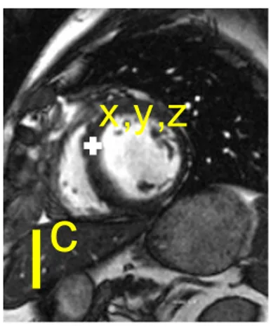
Zhou et al. (2012) showed that where the DICOM orientation (0020,0037) tag is present we can use it to predict the cardiac image acquisition plane (seeFigure 2.3). This tag is not defined as a cardiac view but as two 3-dimensional vectors defining orientation of the imaging plane with respect to the MR scanner coordinate frame.
Figure 2.3: Tips of DICOM plane normals for different cardiac views. In our dataset, distinct clusters can be observed (best viewed in colour). Nevertheless, the separa-tion might not be the case for a more diverse collecsepara-tion of images. Moreover, as we cannot always rely on the presence of this tag an image-content-based recogniser is necessary.
It is straightforward to compute the 3-dimensional normal vectors of this plane as a cross-product of these two vectors specified in the tag. We then feed these three-dimensional feature vectors into any classifier, in our case a classification forest (see Section 2.5.1 for more details on classification forests). This method is shown in the results section as Plane normal + forest.
2.4.1 From DICOM metadata towards image content
This method uses feature vectors computed from the DICOM orientation tag and cannot be used in the absence of this tag. This happens for example in DICOM tag removal after an incorrectly configured anonymisation procedure, when parsing images from clinical journals or when using image formats other than DICOM. In these cases we have to rely on recognition methods using exclusively the image content.
In the next two sections, we present two such methods. One that is based on classification forests and image miniatures (Margeta et al., 2014) and the other one is using CNNs. We learn to predict the cardiac views from 2D image slices individually, rather than using 2D + t, 3D or 3D + t volumes. This decision makes our methods more flexible and applicable also to view recognition scenarios when only 2D images are present, e.g., when parsing clinical journals or images from electronic publications.
2.5
View recognition from image miniatures
Miniatures + forest
First, we propose an automatic cardiac view recognition pipeline (seeFig. 2.4) that learns to recognise the acquisition planes directly from CMR images by combining image miniatures with classification forests.
2.5.1 Decision forest classifier
Decision forest classifier or classification forest (Ho,1995;Amit and Geman,1997;
Breiman, 1999) is an ensemble machine learning method that constructs a set of binary decision trees with split decisions optimised for classification. This method is computationally efficient and allows automatic selection of relevant features for the prediction.
The decision forest framework itself is also quite flexible (Criminisi et al.,2011b;
Pauly,2012) and has already been used to solve a number of problems in medical imaging. For example, for image segmentation (Geremia et al., 2011), organ de-tection (Criminisi and Shotton, 2011;Pauly et al., 2011), manifold learning (Gray et al.,2011), or shape representation (Swee and Grbić,2014).
2.5. View recognition from image miniatures 25
Crop central square
Classification forest
Jitter (translate, rotate, scale)
and crop training slices
Minia
tures
and
int
ensit
y
pool
ing
T
rain
ing
T
est
ing
2 CH 3 CH 4 CH S A X 2 CH 3 CH 4 CH S A X 2 CH 3 CH 4 CH S A X L V OT L V OT L V OTFigure 2.4: Discriminative pixels from image miniatures are chosen from a random pool as features for a classification forest. We jitter the training dataset to improve robustness to differences in the acquisitions without the need for extra data. Training phase
During the training phase, the tree structure is optimised with a divide and conquer strategy on the collection of data points X by recursively splitting them into the left and right branches. This splitting is done such that points with different labels get separated while the same label points are grouped together, i.e., the label purity in the branches increases. SeeFigure 2.5for an illustration of this process.
At each node of the tree a feature from a randomly drawn subset of all features and a threshold value are chosen such that class impurity I in both branches is minimised. We weight samples from the under-represented views more (inversely proportionally to dataset view distribution) and normalise them to sum to one at each node.
I(X, θ) = wlef tH(Xlef t) + wrightH(Xright) (2.1)
H is weighted entropy and Xlef t and Xright are point subsets falling to either the
left or the right branch, based on the tested feature value and threshold. wlef t,
wright are sums of sample weights at each branch and wk is the sum of weights for
a particular class k in the branch. H(X) = −
K
∑
k=1
wklog(wk) (2.2)
Only a random subset of features (e.g. components of the 3D plane orientation vector or a set of pixel intensity values at different fixed locations of the images) is tested at each node of each tree and a simple threshold on this value is used to divide the data points into the left or the right partition. This helps to make the trees in the forest different from each other which leads to better generalisation.
0 1 3 4 5 6 2 S A X 2CH 3CH 4CH L V O T S A X 2CH 3CH 4CH L V O T S A X 2CH 3CH 4CH L V O T S A X 2CH 3CH 4CH L V O T θ1 θ2 5 6 3 4 θ1>T0 θ1>T0 θ1>T0 θ2>T1 θ2>T2 T0 T1 T2
Figure 2.5: We illustrate a 2D feature space and a single tree from the classification forest. At the training phase, the feature space (for example constructed by sam-pling image miniature intensities at random locations) is recursively partitioned (horizontal and vertical lines cut through the feature space) to recognise cardiac planes of acquisition. Class distributions at the leaves are stored for the test time. At the test time, the tested images are passed through the decisions of each tree until they reach the final set of leaves (one per tree). Class with maximal average probability across the forest is chosen as the prediction.
When classifying a new image, features chosen at the training stage are extracted and the image is passed through the decisions of the forest (fixed in the training phase) to reach a set of leaves. Class distributions of the reached leaves are averaged across the forest and the most probable label is selected as the image view. For excellent in-depth discussions on decision forests, in particular applied to medical imaging, see (Criminisi et al.,2011b;Pauly,2012).
2.5.2 Alignment of radiological images
The radiological images are mostly acquired with the object of interest in the image center and some rough alignment of structures can be expected (see Figure 2.6).
Note the large bright cavity in the center (3CH, 4CH), dark lung pixels just above the cavity (SAX), or black air pixels on the left and right side (2CH, SAX). Image intensity samples at fixed positions (even without registration) provide strong cues about the position of different tissues.
2.5.3 Pooled image miniatures as features
It has been shown byTorralba et al. (2008) that significantly down-sampled image miniatures can be used for image recognition. In our case, we extract the central square from each image, resample it to 128 × 128 pixels (with linear interpolation), and linearly rescale to an intensity range between 0 and 255. We subsample the
2.5. View recognition from image miniatures 27
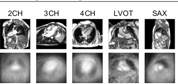
2CH
3 CH
4 CH
LVOT
SAX
Figure 2.6: Example of each cardiac view used in this work (above) and correspond-ing central square region mean intensities across the whole dataset (below).
cropped centers to two fixed sizes (20 × 20 and 40 × 40 pixels). In addition, we divide the image into non-overlapping 4 × 4 tiles and for each of these tiles compute the intensity minima and maxima (seeFigure 2.7).
Image tiles
miniatures
min and max pool
40x40
20x20
32x32
32x32
128x128
(4x4 tiles)Figure 2.7: Image miniatures features: downsampled images and tile intensity min-ima and maxmin-ima are used.
This creates a set of pooled image miniatures (32 × 32 pixels each). The pool-ing adds some invariance to small image translations and rotations (whose effect is within the tile size). The pixel values at random positions of these miniature channels are then used directly as features.
In total 64 random locations across all four miniatures channels are tested at each node of each tree when training the forest. The location and threshold value combination that best (Eq. (2.1)) partition the data-points are then selected and stored and the data points are correspondingly divided into the left and right
branches. We recursively continue dividing the dataset until not less than 2 points are left in each leaf or no gain is obtained by further splitting. We trained 160 trees in total using Scikit-learn (Pedregosa et al.,2011).
This method is shown in the evaluation as Miniatures + forest.
2.5.4 Augmenting the dataset with geometric jittering
While the object of interest is in general placed at the image center, some differences between various imaging centres and positioning of the heart on the image remain (see Fig. 2.12). The proposed miniature features are not fully invariant to these changes per se. To account for larger differences in acquisition we augment the training set (artificially increase its size) with extra images created by transforming the originals. In other words, we artificially generate new images from the originals by geometric transformations. It makes sense to perform appearance transforma-tions as well (e.g. intensity alteratransforma-tions done byWu et al.(2015) or adding synthetic bias fields). Only care must be taken not to modify the target label. The advantage of data augmentation is that very realistic images can be obtained without extra acquisition or labelling cost. The downside is that excessive augmentation makes the images look more alike and there is a greater risk of overfitting to the training set.
For our purpose, we augment the dataset on a regular grid of transformation parameters. These were translations (all shifts in x and y between -10 and 10 pixels for a 5 × 5 grid), but also scale changes (1 − 1.4 zoom factor with 8 steps while keeping the same image size) and in-plane rotations around the image cen-tre (angles between -10 and 10 degrees with 20 steps). The augmented images were resampled with linear interpolation. Note that the extra expense of dataset augmentation is present mainly at the training time as more data points are used. The test time remains almost unaffected, however, now a deeper forest could be learnt. As we will see later in the results, the benefit of dataset augmentation for this forest-based method is clear, yielding a solid 12.14% gain in the F1 score (F 1 = 2(precision.recall)/(precision + recall)). Results using this augmented dataset are presented in the evaluation as Augmented miniatures + forest.
2.5.5 Forest parameter selection
We first trained and tested this forest-based algorithm on a subset of our dataset con-sisting of 960 image slices from 100 cardiac patients (SAX: 540, 4CH: 140, 2CH: 112, 3CH: 107, LVOT: 9) coming from the DETERMINE study (Kadish et al., 2009) and obtained via the Cardiac atlas project infrastructure (Fonseca et al., 2011) (www.cardiacatlas.org). Through the augmentation we obtained 51894 training images in total.
We ran a 25-fold cross validation by dividing the dataset on patient identifiers to prevent biasing our results due to repeated view acquisitions and other acquisition similarities. This means that images from the same patient (despite being from