Prediction of U.S. General Aviation fatalities from extreme value approach

O

pen

A

rchive

T

oulouse

A

rchive

O

uverte

(OATAO)

OATAO is an open access repository that collects the work of some Toulouse

researchers and makes it freely available over the web where possible.

This is

an author's

version published in:

https://oatao.univ-toulouse.fr/22976

Official URL :

https://doi.org/10.1016/j.tra.2018.01.022

To cite this version :

Any correspondence concerning this service should be sent to the repository administrator:

tech-oatao@listes-diff.inp-toulouse.fr

Diamoutene, Abdoulaye and Kamsu-Foguem, Bernard and Noureddine, Farid and

Barro, Diakarya Prediction of U.S. General Aviation fatalities from extreme value approach.

(2018) Transportation Research Part A: Policy and Practice, 109. 65-75. ISSN 0965-8564

OATAO

Prediction of U.S. General Aviation fatalities from extreme value

approach

Abdoulaye Diamoutene

a,b,c

, Bernard Kamsu-Foguem

a,⁎

, Farid Noureddine

a

,

Diakarya Barro

c

a_{Université de Toulouse, Laboratoire de Génie de Production (LGP), EA 1905, 47 Avenue d’Azereix, BP 1629, 65016 Tarbes Cedex, France} b_{Institut Polytechnique Rural de Formation et de Recherche Appliquée de Katibougou Mali, BP: 06 Koulikoro, Mali}

c_{Université Ouaga 2, UFR-SEG, 12 BP: 417 Ouagadougou 12, Burkina Faso}

A R T I C L E I N F O

Keywords:

General Aviation accident Extreme value statistics Graphical diagnosis Return level Uncertainty

Nonparametric bootstrap

A B S T R A C T

General Aviation is the main component of the United States civil aviation and the most aviation accidents concern this aviation category. Between early 2015 and May 17, 2016, a total of 1546 general aviation accidents in the United States has left 466 fatalities and 384 injured. Hence, in this study, we investigate the risk of U.S. General Aviation accidents by examining historical U.S. General Aviation accidents. Using the Peak Over Threshold approach and Generalized Pareto Distribution, we predict the number of fatalities resulting in extreme GA accidents in the future operations. We use a graphical method and intensive parameters estimates to obtain the optimal range of the threshold. In order to assess the uncertainty in the inference and the accuracy of the results, we use the nonparametric bootstrap approach.

1. Introduction

General Aviation (GA) is the term for all civil aviation operations other than scheduled air service and non scheduled air transport

operations for remuneration or hire, seeCrane (1997)and National Transportation StatisticsNTS (2016). GAflights range from

gliders and powered parachutes to corporate business jetflights, see National Transportation Safety BoardNTSB (2011)and Civil

Aviation AuthorityCAA (2013). The majority of the world’s air traffic falls into this category and most of the world’s airports serve

general aviation exclusively, seeCrane (1997). The term General Aviation is a catch all phrase for all aviation activities that do not

fall under commercial aviation, major cargo or military operations, and covers a broad spectrum of aviation activity uses. Between early 2015 and May 17, 2016, a total of 1546 general aviation accidents in the United States has left 466 fatalities and 384 injured, according to data from the NTSB.

In 2011, GA aircrafts were involved in 95% of all aviation accidents and 94% of fatal aviation accidents; accidents involving GA

aircrafts accounted for 92% of all U.S. civil aviation fatalities, seeNTSB (2011); it is an important component of civil aviation in the

United States, seeShetty and Hansman (2012).

GA covers a large range of activities, both commercial and non commercial, includingflying clubs, flight training, agricultural

aviation, light aircraft manufacturing and maintenance. GA is particularly popular in North America, with over 6,300 airports

available for public use by pilots of GA aircraft in the U.S., seeNTSB (2011)andNTS (2016).

In 1990 2014, there is in United States GA a total of 8402 fatal accidents which resulted in about 14984 fatalities according to data from the National Transportation Safety Board (NTSB). Among these 8402 fatal accidents, around 26 accidents can be

⁎_{Corresponding author.}

considered as extreme and each of them was responsible for more than 39 fatalities. Moreover, in extreme value approach, an extreme event is an event which has a low probability, but implies serious consequences. In our context, an extreme accident is an

accident that has caused over 39 fatalities. Although there is an overall decreasing trend in the annual number of fatalities, seeNTS

(2016)andShetty and Hansman (2012), there is no such trend in the number of extreme fatal accidents which cause enormous fatalities. Prediction and risk management in terms of extreme fatality are more important in insurers, reinsurers and aeronautics

industry like Boeing and Airbus, seeBoeing (2016)andAirbus (2016). Moreover, based on historical data, the return level of fatalities

could help management agency of GA to perform aircraft operations, conditions based maintenance, predictive maintenance and flying conditions.

The safety of civil aviation in the United States is regulated by the Federal Aviation Administration (FAA), for more details see

NTSB (2011). The FAA distinguishes between commercial operations and GA operations, seeNTSB (2011). There are other orga nizations like International Civil Aviation Organization (ICAO), Civil Aviation Authority (CAA) of the United Kingdom (UK) and leading manufacturers of commercial jetliners such as Boeing, Airbus give valuable reports on civil aviation accident. These reports

mainly focus on descriptive accident statistics such as the rate of fatal accidents, fatalities by year, nature offlight, type of aircraft,

transport category,flight hours, for more details, seeNTSB (2011)andNTS (2016).

In literature, some works on aviation accidents focus on the cost of GA accidents in U.S., seeSobieralski (2012); Knetch (2015)

focuses on the prediction of the accident rate due to pilot totalflight hours;Fultz and Ashley (2016), study extreme weather impact in

GA accidents in the United States;Farah and Azevedo (1952)focus on safety analysis of passing maneuvers using extreme value

theory.Sha et al. (2017)focus on the use of the extreme value theory for forecasting spare parts stocks on the basis of repair data set

information, seeRomeijnders et al. (2012).Dey and Das (2016)propose an approach to predict extreme aviation fatal injuries. But in

literature, it is rare to see research concerning the modeling of the number of fatalities in individual U.S. GA accidents; using extreme value models, notably Peaks Over Threshold (POT) approach. From extreme value statistics, we can model the return level of fatalities due to extreme GA accidents. We distinguish two approaches namely, block maxima approach and Peak Over Threshold

(POT) approach, seeColes (2001). The block maxima approach is wasteful of data as only one data point in each block is taken. The

second highest value in one block may be larger than the highest of another block and this is generally not accounted for, seeColes

(2001) andCastillo et al. (2005). Peak Over Threshold (POT) approach avoids this drawback, by using the Generalized Pareto Distribution (GPD). Indeed, due to advances in extreme value theory, the GPD emerged as a natural family for modeling exceedances over a high threshold. The POT approach has shown its importance and success in a number of statistical analysis problems related to

different areas, seeSchmidt et al. (2014)andCastillo et al. (2005). However, despite the sound theoretical basis and wide applic

ability, thefitting of this distribution in practice is not a trivial exercise.

In this paper we focus on U.S. GA fatal accidents from 1990 to 2014 and their resulting fatalities number. A prediction of the possible number of fatalities for an extreme GA accident in the future operation is made using POT approach. We use three estimation methods to estimate the parameters and select the method which standard error is less than in the other two methods. The two main factors which affect the accuracy of the estimations of the return values are the choice of the threshold on one hand and the choice of the parameter estimator on the other hand. An extensive discussion of the various parameter estimation methods has been given by

Bermudez and Kotz (2010).Scarrot and Macdonald (2012)reviewed the threshold estimation methods; hence, we use graphical method and intensive estimate of GPD parameters to obtain a reasonable range of the threshold. We also quantify the uncertainty in

the inference using nonparametric bootstrap approach, seeCarpenter and Bithel (2000)andYongcheng (2008).

This paper is structured as follows: following this introduction, Section 2provides background on extreme values statistics,

notably both block maxima approach and POT approach. Section3exposes GA accident modeling with POT approach. Section4

presents different uncertainty measurements in the inference of U.S. GA extreme fatalities and finally Section5concludes and

discusses future challenges.

2. Extreme value theory

Most statistical methods are concerned primarily with what goes on in the center of a statistical distribution, and do not pay particular attention to the tails of a distribution, or in other words, the most extreme values at either high or low end. However, in extreme value analysis, we are not interested in estimating the average we rather want to quantify the behavior of the process at

unusually large or small levels, seeColes (2001). Extreme Value Theory (EVT) deals with the extreme deviations from the median of

probability distributions and seeks to assess, from a given ordered sample of a given random variable, the probability of events that

are more extreme than a certain large value, seeColes (2001)andCastillo et al. (2005).

Broadly speaking, there are two principal kinds of models for extreme values. The first group of model, called Generalized

Extreme Value theory (GEV) consists of block maxima approach; these are models for the largest observations collected from large samples of identically distributed observations. A second group of EVT models contains the Peak Over Threshold (POT) models,

which model all large observations that exceed a high threshold, for more details seeColes (2001)andCastillo et al. (2005). These

POT models are generally considered to be most useful for practical applications, due to their more efficient use of the (often limited)

data of extreme values. Within the POT class of models, several styles of analysis exist, seeColes (2001)andSchmidt et al. (2014).

Among all these parametric models, the Generalized Pareto Distribution (GPD) has the advantage of being conceptually simple and

2.1. Block maxima approach

Let X X1, , ,2…Xn be a sequence of independent and identically distributed (i.i.d) random variables with common distribution

function F. Extreme value analysis focuses on the statistical behavior of the maximum value observed, i.e.,Mn=max X X{ , , ,1 2…Xn}.

In applications, the Xi usually represent values of a process measured on a regular time scale at time i such as the hourly

measurements of sea level, or daily mean temperature so that Mn represents the maximum of the process over n time units of

observation, seeColes (2001). If n is the number of observations in a year, thenMncorresponds to the annual maximum. Using the

fact thatX X1, , ,2…Xnare i.i.d random variables

⩽ = ⩽ … ⩽ = ⩽ ×…× ⩽ = Pr M x Pr X x X x Pr X x Pr X x F x ( ) { , , } { } { } { ( )} . n n n n 1 1

In practice, we might not know the distribution function F but according to the extremal type, if there exist sequences of constants >

a

{ n 0}and b{ }n such thatPr

{

(

Mn_a−_nbn

)

⩽x

}

→G x( )asn→ ∞with G being a non degenerate distribution function, then G belongs to

the following family of models having a distribution function of the form:

= ⎧ ⎨ ⎩ −⎡ ⎣ + ⎛⎝ − _⎞ ⎠ ⎤ ⎦ ⎫ ⎬ ⎭ − G x ξ x μ σ ( ) exp 1 ξ , 1 (1) defined on the set

{

z: 1+ξ

( )

x−μ >0

}

σ , where the parameters satisfy −∞ <μ< ∞,σ>0 and −∞ <ξ< ∞. This is the generalized

extreme value family of distributions. The model has three parameters: a location parameter μ; a scale parameter σ ; and a shape

parameterξ. The shape parameterξgoverns the tail behavior of the distribution. The sub families defined by →ξ 0,ξ>0 andξ<0

correspond, respectively to Gumbel, Fréchet and Weibull families, for more details seeColes (2001).

2.2. Peak over threshold approach

Compared to the traditional approaches, the POT method can utilize more information from the data set. In contrast to block maxima approach, it is more practical to analyze the value of random variables that exceed a given threshold value if an entire time

series of, say, hourly or daily or yearly observations is available, this method is commonly known as POT approach, seeFar and

Wahab (2016)andCastillo and Daoudi (2009). Hence, the POT approach provides a more rational selection of events fulfilling the

criteria of being“extreme”. In this approach observations that exceed a given threshold μ are called exceedances over a threshold.

POT method has popularly been used to estimate return levels of significant wave height, seeMackay et al. (2014), hurricane damage

inDaspit and Das (2012), Schmidt et al. (2014)in the study of traffic load effects on bridges and earthquakes modeling inEdwards and Das (2016).Pickands (1975)proves that for large enough threshold μ, observations x, providedx>μ, approximatively follow a Generalized Pareto Distribution (GPD) with distribution function:

= ⎧ ⎨ ⎪ ⎩ ⎪ − + ≠ > − − = > − − −

(

)

(

)

F x ξ σ ξ σ ( ) 1 1 , 0, 0, 1 exp , 0, 0. ξ x μ σ ξ x μ σ ( ) 1 (2)

The GPD defined in Eq.(2)reduces to a 2 parameter GPD forμ=0and for most of the practical purposes the 2 parameter GPD

seems more appropriate than the 3 parameter GPD as described inFar and Wahab (2016), so in our study, a 2 parameter GPD is

considered. For different values of the shape parameter, GPD provides few interesting distributions. For <ξ 0, the distribution has a

heavy Pareto type upper tail. Forξ=0, the GPD provides the exponential distribution with mean σ . Forξ=0.5andξ=1the

distribution is triangular and uniform respectively. When ⩽ξ −1

2,Var X( )= ∞, and the rth central moment exists if and only if ⩾ −

ξ

r

1

. The GPD is stable with respect to excesses over threshold operations. In other words, if the random variable X has a generalized Pareto withGPD ξ σ( , ), then the conditional distribution of(X μ− ) subject toX⩾μis also generalized Pareto withGPD ξ σ( , +ξμ) and

so the new GPD retains the same shape parameter valueξand this property is known as the threshold stability property as shown in

Mackay et al. (2014).

2.3. Graphical diagnosis for threshold choice

The threshold stability property of GPD means that if the GPD is a valid model for excesses over thresholdμ₀, then it is valid for

excesses over all thresholdsμ₀, the expected value of our threshold excesses, conditional on being greater than the thresholdμ₀, is

− > = + − E X μ X μ σ ξμ ξ [ | ] 1 . μ0

Thus, for allμ>μ E X μ X₀, [ − | >μ], is a linear function of μ. Futhermore,E X μ X[ − | >μ] is simply the mean of the excesses of threshold μ, for which the simple mean of the threshold excesses of μ provides an estimate. This leads to the mean residual life plot (mrlplot) or mean excess plot (meplot), a graphical procedure for identifying a suitably high threshold for modeling extremes via the

GPD. In this plot, for a range of candidate values for μ, we identify the corresponding mean threshold excess; we then plot this mean

threshold excess against μ, and look for valueμ₀above which we can see linearity in the plot, for more details seeRibatet (2012)and

Scarrot and Macdonald (2012).

2.3.1. Mean excess plot and mean residual life plot

The observations exceeding a given threshold μ in the tail of the distribution approximately follow GPD. However, a crucial step in this analysis is to select an appropriate threshold μ. On one hand, if μ is too small, then the GPD will notfit the tail distribution and

the estimates of parameters ξ σ( , )may be biased. On the other hand, if μ is too large, the GPD mayfit well, but fewer observations will

be available to estimate the parameters and the estimates will suffer from increased variance. We want to select the smallest μ in

mrlplot and meplot (Fig. 3) above which the mrplot and meplot will be approximately linear.

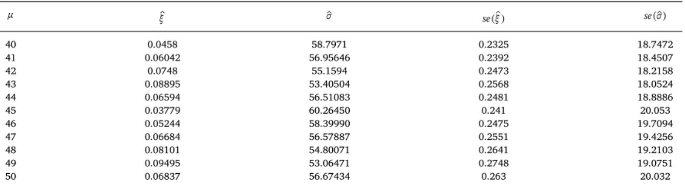
2.3.2. Parameter stability plot

A common diagnosis is the threshold stability plot where estimated shape parameters (including pointwise uncertainty intervals) are plotted against a range of possible thresholds. The threshold is chosen as the lowest possible value such that the shape parameter

is stable for all higher values, once sample uncertainty is taken into account. A similar plot of modified scale parameter estimated is

occasionally considered, although the correlation between scale and shape parameter is often not obvious.

In practice, threshold μ should be chosen where the shape and modified scale parameters remain constant in parameter stability plot after taking the sampling variability into account.

2.4. Return period and return level estimation

In extreme value statistics it is common to use the notion of return period and return level to interpret and explain the information

about the likelihood of extreme events such asfloods, earthquakes, hurricanes, aviation accidents, etc. An estimate of the t ob

servations return level xt that is exceeded on average once every t observations is given by

̂ ̂ ̂ ̂ =⎧ ⎨ ⎩ + − ≠ + = x μ tλ for ξ μ σlog tλ for ξ [( ) 1] 0 ( ) 0, t σ ξ μ ξ μ    (3) provided that t is sufficiently large to ensure thatxt >μ.

An estimate ofλμ, the probability of an individual observation exceeding the threshold μ, is also needed. The natural estimator of

λμis λ=μ _nk, the sample proportion of points exceeding μ. Since the number of exceedances of μ follows the binomial Bin n λ( , )μ

distribution, λ is also the maximum likelihood estimate ofμ λμ, seeColes (2001).

By construction, xtis the t observation return level; however, it is often more convenient to give return levels on an annual scale,

so that the T year return level is the level expected to be exceeded once every T years. If there are nyobservations per year, this

corresponds to the t observation return level with =t T×ny. Hence, an estimate of theT−year return levelxTis defined by

̂ ̂ ̂ = ⎧ ⎨ ⎩ + − ≠ + = x μ T n λ for ξ μ σlog T n λ for ξ [( . ) 1] 0 ( . . ) 0, T σ ξ y μ ξ y μ    (4) provided that t is sufficiently large to ensure thatxT >μ.

Estimation of return levelsxT requires the substituton of the estimates of the different parameters and likelihood estimate ofλμ.

In the remainder of this document, the return period T corresponds to the period of prediction in terms of years and the return

levelxT is the possible prediction of fatalities according to model parameters.

3. Modeling of U.S. General Aviation fatalities 3.1. Data presentation

The purpose of this study is to develop a predictive model which will provide estimates of potential fatalities for an extreme aviation accident in the future of U.S. GA. Data are obtained from U.S. General Aviation safety data which is a division of the National Transportation Safety Board (NTSB). The NTSB aviation accident database contains information within the United States, its terri tories and possessions and in international waters. The data consist of 8402 U.S. GA fatal accidents from 1990 to 2014 which caused in total about 14984 fatalities. U.S. registered civil aircrafts are not operated under 14 CFR 121 or 14 CFR 135. Accidents on foreign soil and in foreign waters are excluded. Suicide, sabotage, and stolen/unauthorized cases are included in total accidents fatalities.

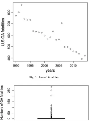
Fig. 1shows the evolution of U.S. General Aviation fatalities from 1990 to 2014. Generally speaking, we observe a diminution of

fatalities over years. However,Fig. 1does not exhibit an individual extreme fatality.

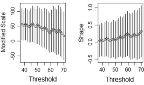
Fig. 2shows the individual assignment of the data; we observe that most fatalities is less than 39.

Figs. 1 and 2show that there is a nuance between the declination trend of annual fatalities and fatalities resulting in individual extreme GA accident.

3.2. Application of graphical approach in the choice of threshold

In this subsection, we use the theoretical approach presented in Section2.3. We would selected the smallest μ in meplot and

mrlplot (Fig. 3) above which the meplot and mrplot will be approximately linear.

Fig. 3shows that the reasonable threshold should be in the range (40 70).

According to theFig. 3, parameter stability plots inFig. 4also suggest selecting the threshold in the range (40 50).

3.3. Fitting the GPD parameter and return levels for different threshold values

Once the threshold value has been specified, estimating the shape and scale parameters would be the next step of developing models. The importance of parameter estimations in POT method cannot be underestimated as they may create errors in estimating

the high quantiles. There are numerous parameter estimation methods available in the literature tofit the GPD parameters to the set

of threshold excesses such as maximum likelihood estimate (MLE), Method of Moment (MOM) and Probability Weighted Moment

(PWM), least squares error method, etc.Dupuis and Tsao (1998)proposed a hybrid estimators of two well known estimators: Method

of Moment (MOM) and Probability Weight Moment (PWM); the methods were derived by incorporating a simple auxiliary limitation

of the estimates. Bermudez and Kotz (2010)carried out an extensive study on several types of methods for estimating the GPD

parameters; the authors argued that the success of GPD on a set data depends substantially on the process of parameter estimates, and Fig. 1. Annual fatalities.

Fig. 2. Boxplot of U.S. GA data.

Fig. 3. Mean excess plot and mean residual life plot.

(J) Q)

:e

ro

]!

,:i:: (9 (f)

:j

(/)

"'

~ ro J§ <( (9 0 (/) li, .0 E :::,

z

(J) (J) Q) u X

w

C (1J Q)

2

0 0 0 - 0 00 0 0 O 0 0 o - 0 ,-. 0 0 0 0 0 0 0 -(0 0 0

-"'

0 o

_....

-1 1 1990 1995 0

"'

-N

-0 ':!2

-0

"'

0

-Mean Excess Plot

0 ~ 0 0 0

o

;~

~

o90

0 (0 @ 0 0 N 0 t} 0 40 80 120

Threshold

0 0 0 oO 0 0 0 Oo 0 0 0 1 1 1 2000 2005 2010

years

0 0 0 €1 ffl

1

Mean Residual Life Plot

(J) (J) Q) u X

w

C (1J Q)

2

0 40 80

Threshold

(MLE) estimators has been the most popular method among other estimators. However, the (MLE) estimators exist only for the shape

parameter ≤ξ 1because forξ>1the log likelihood becomes infinite. In this study, the estimation of GPD parameters and adequate

threshold choice are performed using the maximum likelihood, Method of Moment and Probability Weighted Moment (PWM).

For maximum likelihood estimate, the GPD log likelihood function forξ ≠ 0can be derived in the usual way as follows:

∑

⎜ ⎟ ⎜ ⎟ = − −⎛ ⎝ + ⎞ ⎠ ⎛ ⎝ + ⎞ ⎠ = + l ξ σ y ne logσ ξ log ξy σ ( , ; ) . 1 1 1 , i ne i 1 (5)

wherey=( , , ,y y1 2…yne)are the set of exceedances above threshold μ. For the case =ξ 0, interpreted as →ξ 0, we have the log likehood for an exponential distribution with rate

σ

1

. In the software R, we could write a function which computes the negative log likehood for

the GPD, and then use the nlme routine to minimize this with respect toθ=( , ). Here, we will obtain maximum likelihood estimatesξ σ

of the GPD parameters for our aviation fatalities by using thefitgpd function in the package POT.

Method of Moment estimates ofξand σ can be easily obtained by using the mean and variance of the exceedances. The estimates

ofξand σ are given by:

̂= ⎛ _̂ ⎝ − ⎞ ⎠ = ⎛ ⎝ + ⎞ ⎠ ξ y s and σ y y s 1 2 1 1 2 1 . 2 2 2 2 ₍₆₎

Probability Weighted Moment (PWM) is based onHosking and Wallis (1987), the general expression for the rth order of PWM of

GPD is given by: = + + + + + M u r σ r r ξ 1 (1 )(1 ). r

The estimate of the rth order of PWM is given by:

∑

= − = M P y k (1 ) r i k i i k 1 2 : 

with plotting positionPi=i−_k0.35. The estimates ofξand σ can be obtained using

̂= _̂ − − = − ξ M M M and σ M M M M 2 2 2 2 , 0 0 0 0 1 0 1        ₍₇₎

for more details seeDupuis and Tsao (1998).

Fig. 4. Parameter stability plot.

Table 1

Parameters estimates in MLE for various thresholds.

μ _ξ̂ σ_̂ se ξ( )̂ se σ( )̂ 40 0.02545 60.21724 0.2449 19.8103 41 0.04654 57.96778 0.2492 19.2504 42 0.06782 55.75671 0.2537 18.7157 43 0.09026 53.5635 0.2592 18.2129 44 0.05335 57.4497 0.2588 19.7149 45 0.01133 62.11331 0.26 21.61 46 0.0328 59.7771 0.2634 20.9387 47 0.05326 57.59795 0.267 20.354 48 0.07631 55.28838 0.2714 19.7162 49 0.1035 52.7837 0.2772 19.0017 50 0.05656 57.59245 0.278 21.043 0 0 Q) 0

ro

u 0 Q) "1 (/) LO 0 . . 0 -0 _Cil Q) ~ ..c -0 0 (/) C) 0 0 ~ 0

"?

"1 9

40

50

60

70

40

50

60

70

Threshold

Threshold

3.3.1. Maximum Likelihood Estimates of GPD parameters for potential thresholds

The parameter values and their standard errors are computed over formula 5 and software R; the results are in theTable 1.

Forξ>0, the distribution has no upper limit, see Coles (2001). The examination of the shape parameter estimates and its

standard error show some level of instability in the shape parameter estimation. In the ranges 40 43 and 45 49, the shape parameter increases and the same for the standard errors, for threshold values 45 and 50 we have the isolate values. We also observe that MLE is sensitive to the threshold choice.

3.3.2. Method of Moment for potential thresholds

Table 2below gives the values and the standard errors of the parameters over formula 6 and software R.

In MOM, the shape parameter is positive showing that the distribution has no upper limit. The examination of the shape para meter estimates and its standard errors show the same results as MLE but the standard error of shape parameter in MOM is less than in MLE.

3.3.3. Method of Probability Weight Moment for potential thresholds

TheTable 3below provides the values and the standard errors of the parameters over formula 7 and software R. Concerning PWM, we have the same variation with a greater standard error for the estimates of the shape parameter. All these methods are sensitive to the threshold choice. The examination on the estimates in the three selected methods shows that MOM and MLE are less sensitive to any change in the value of threshold than PWM. In the following, we use MLE and MOM because their standard errors are less high than in PWM.

3.3.4. General Aviation fatalities return level estimates for the potential thresholds

In this subsection, we use the estimates of the parameters fromTables 1 and 2for the threshold value 40, 45 and 50 to calculate

the return level of fatalities for the periods 5, 10 and 25 years. By replacing in Eq.(4), the estimates of parameters and return period,

we obtain theTable 4below.

Table 4summarizes the T year return levels for different values of T and the two methods used. The examination of the results in

Table 4shows that for each return period, the estimates of return levels are almost the same for the two different methods (MLE and

MOM). However, from threshold 45 to threshold 50, we note that there is a very little change in fatalities number. This means that the optimal range of threshold is range 45 50. For example, with MOM 5 year return level is 139 fatalities for threshold 45, that implies that about 139 fatalities are likely to occur once in every 5 years. Another interpretation for 5 year return level for threshold 45 with 2014 as reference year, is that in 2019 a possible number of fatalities is 139. General Aviation accidents factors such that technology,

Table 2

Parameters estimates in MOM for the various thresholds.

μ _ξ̂ σ_̂ se ξ( )̂ se σ( )̂ 40 0.0458 58.7971 0.2325 18.7472 41 0.06042 56.95646 0.2392 18.4507 42 0.0748 55.1594 0.2473 18.2158 43 0.08895 53.40504 0.2568 18.0524 44 0.06594 56.51083 0.2481 18.8886 45 0.03779 60.26450 0.241 20.053 46 0.05244 58.39990 0.2475 19.7094 47 0.06684 56.57887 0.2551 19.4256 48 0.08101 54.80071 0.2641 19.2103 49 0.09495 53.06471 0.2748 19.0751 50 0.06837 56.67434 0.263 20.032 Table 3

Parameters estimates in PWM for the different thresholds.

μ _ξ̂ σ_̂ se ξ( )̂ se σ( )̂ 40 0.04856 58.62684 0.2509 19.5998 41 0.08023 55.75563 0.2513 18.6905 42 0.1119 52.9478 0.2528 17.8111 43 0.1436 50.2032 0.2554 16.9630 44 0.09243 54.90782 0.2579 18.8842 45 0.02799 60.87868 0.264 21.367 46 0.05947 57.86614 0.2638 20.3908 47 0.09096 55.11657 0.2646 19.4454 48 0.1224 52.33 0.2665 18.5319 49 0.1539 49.6064 0.2698 17.6514 50 0.09409 55.10938 0.272 19.982

Table 4

Estlmates ,:J fatalltles expected to be exceeded once every T years.

5years l0years 25years

µ Fat.MU! Fat.MOM µ Fat.MU! Fat.MOM µ Fat.MU! Fat.MOM

40 133 132 40 177 177 40 236 238

45 140 139 45 184 183 45 243 245

50 141 141 50 186 185 50 247 248

traffic management and flying conditions permit to maintain the mode! U$ed in

this

study,

4. Uncertainty quantification

In the area of insurers and reinsurers, the management and prediction of extreme risk events like aviation accidents fatalities is

very important. However, most mathematical models do not provide a perfect representation of reality; the adequacy of model and

inference of models parameters are often uncertain. Thus, taking into account assessing uncertainties is very important when we

extrapolate the observed data.

In literature, several methods (graphical and numerical) have been proposed to assess <lifferent sources of unœrtainties in the

extreme value statistics, for more details see Wehner (2010), Scarrot and Macdonald (2012), Zhang et al. (2015) and Wendy and

Noriszura (2012). In this work, we focus on uncertainties in model adequacy and model parameters due to threshold selection.

4.1.

Uncertninty from model adequacy

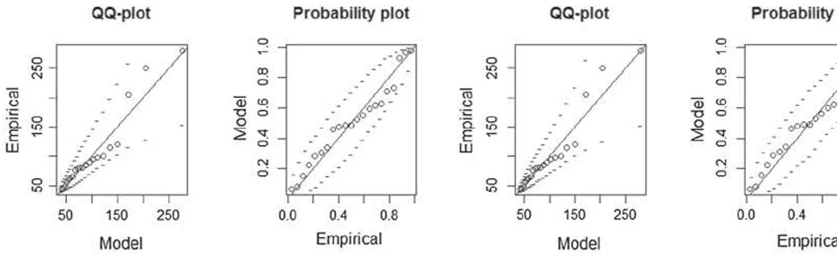
We use quantile plot and probability plot to check the suitability of the fitted GPD to the set of extracted threshold exœedances.

The analysis of the previous section has shown that the standard error of shape parameter in MOM and MLE are Jess than the standard

error in PWM; For that reason, we consider MOM and MLE methods in our analysis. We use the graphical approach to quantify

unœrtainty from mode! adequacy; the

QQ

plots and PP plots are done for MLE and MOM estimates for the threshold range 40 50,

specifically for the threshold values 40, 45 and 50.

Figs. 5 and 6 show the QQ plot and PP plot for thresholds 40 and 45 in MLE Oeft) and MOM (right); in MLE,

QQ

plot has a clear

deviation from 45 degree line. In MOM, QQ plot is 45 degree line and PP plot is 45 degree line in both methods.

Fig. 7 shows that

QQ

plot and PP plot are 45 degree line in both methods. The synthesis of graphical analysis shows that ail

QQ

plots and PP plots for MOM are 45 degree line; this means that MOM is more sui table in this work. In the following, ail the estimates

are done with MOM estimator.

4.2.

Uncertninty from estimate of the model paramew-s

The main source of uncertainty in quantifying extreme events such extreme aviation fatalities with GPD is the choice of the

threshold. In this work, we use graphical method and intensive parameter fitted with MLE, MOM and PWM to select the appropriate

range for threshold and to obtain the optimal threshold. There are some tools to measure the uncertainty in fitted GPD like coefficient

of variation (CV), standard error (SE), confidence level of the parameter of interest. In our approach, for each potential threshold,

standard error of shape and scale parameter are computed. The results obtained suggest that MLE and MOM are sui table than PWM to

fit GPD parameter. In the previous section, Table 4 summarizes the estimates of an T return level for <lifferent levels and two selected

methods. Here, in order to quantify the uncertainties in parameter estimates, we investigate the basis of their standard error,

coefficient of variation and confidence intervals. However, a standard 95% confidence interval for level

x

r

depends on the asymptotic

normality of~ -This asymptotic normality assumption is not always proven out in practice for data with small observations, see

QQ-plot Probability plot QQ-plot Probability plot

~ ~ 0 0

.,,

0 _~

.,,

0 (X)

"'

0 _o·

"'

ci ni 0 o. ni 0 u QÏ <D _<FP.· u QÏ <D ·.::: 'O ci ·::: 'O ci 'êi 0

.,,

_{0 "ëi.} 0 ₀ •n E ~ 2 <i: _{E 2} <i: w 0 _w 0

"'

"'

0 0 0

.,,

0

.,,

50 150 250 0.0 0.4 0.8 50 150 250 0.0 0.4 0.8

Model Empirical Model Empirical

Carpenter and Bithel (2000)andNaess and Clausen (2001). We want to construct a confidence interval without taking into account

this assumption. Hence, we use nonparametric resampling (nonparametric bootstrap) which makes no assumption concerning of model. Our data is assumed to be a vector zobsof n independent observations, and we are interested in a confidence interval forθzobs.

The general algorithm for a nonparametric bootstrap is as follows:

1. Sample n observations randomly with replacement from zobsto obtain a bootstrap data set, denotedZ∗. However, in our case the

original data set consists of number of observations with exceedances above the selected threshold. A random sample size number of exceedances is selected with replacement from the original data set to obtain a bootstrap data set. From this bootstrap data set

MOM estimates of parameters are calculated and using these estimates the return levelxTis determined for each return period

=

T 5,T=10 andT=25.

2. Calculate the bootstrap version of the statistic of interest,_θ∗=_{θ Z(} ∗_).

3. Repeat steps 1 and 2 a large number of times, say B, to obtain an estimate of the bootstrap distribution.

In our simulation,B=1000, the statistic of interest is return levelxT, shape parameterξand scale parameter σ .

The procedure is repeated 1000 times; for each return period( )T we have 1000 values of return level. Using this set of 1000 values

the mean return fatalities, standard error, coefficient of variation, minimum and maximum fatalities are calculated for thresholds 40,

45 and 50. The results are summarized inTables 5 7.

The examination of results in Tables 5 7shows that the standard error, the coefficient of variation, the minimum and the

maximum fatalities for return level increase with the return period. This means that the uncertainties increase with the return period. We also note that there is no significative difference between the results of thresholds 45 and 50; this implies that the model gives almost similar results for any threshold value between 45 and 50. According to model adequacy and nonparametric bootstrap approach, we can say that the optimal threshold is around 45.

Results inTable 8show that the root mean square error (rmse) for the parameter estimates (shape and scale) are almost the same.

Fig. 6. QQ-plot and PP-plot for MLE (right) and MOM (left) with thres. = 45.

Fig. 7. QQ-plot and PP-plot for MLE (right) and MOM (left) with thres. = 50.

Table 5

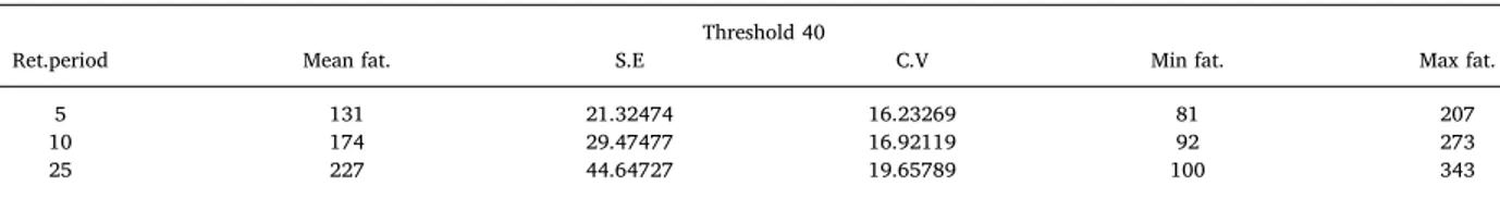
Mean fatalities, standard error, coefficient variation, min fatalities, max fatalities from bootstrap resampling (threshold 40). Threshold 40

Ret.period Mean fat. S.E C.V Min fat. Max fat.

5 131 21.32474 16.23269 81 207

10 174 29.47477 16.92119 92 273

25 227 44.64727 19.65789 100 343

QQ-plot Probability plot QQ-plot Probability plot

q q --·o -- 0 0 (D 0 _~ 6 0

ro

0 ₀ • -

ro

0 _{0 oO_} 0 o_ 0 0 N _ai <D 0 N Q) <D

·

=

_-0 6 ooo_ - -0 6 oO -0 -ë5. 0 0 - ëï 0 E 2 si: - 0 E 2 si: • -• w 0 00 - 0 w 0 0~ - 0 ~ <'! -•o ~ <'! ·ooo 0 -0 0 -• 0 ₀ 0 ₀

"'

"'

50 150 250 _0.0 0.4 0.8 50 150 250 0.0 0.4 0.8

Madel Empirical Model _Empirical

QQ-plot Probability plot QQ-plot Probability plot

q q - -0 ---o 0 _~ 0 _~ 0 0

ro

0 0 00_

ro

0 0 oO_ 0 0 _Q) <D 0 0 Q) U) ·c N -0 6 ooo_ ·c N -0 6 oo

-·

o.

0

·

o.

0

E 2 si: _-•o E 2 si: -•o

w 0 00 - 0 w D 0 0 N ~ N - Q 6 -•O 6 -00 0 0 D 0

"'

"'

50 150 250 0.0 0.4 0.8 50 150 250 0.0 0.4 0.8

The same goes for the return level estimates. This analysis confirms the results inTables 5 7; thus we can observe that there is no misspecification problem due to the threshold range selection of the model around threshold value 45.

4.3. Comparison between return level with original data and simulated data

In the resampling procedure, the original data set consists of number of exceedances above the thresholds 40, 45 and 50. A sample of size of exceedances number is selected with replacement from the original data set to obtain a bootstrap data set. The entire number of fatalities above the selected threshold changes with replacement. Thus, the expected values and the mean values from the

bootstrap must be in 95% bootstrap confidence intervals to obtain accurate results.

According toTables 5, 6, 7 and 9, we observe that the mean fatalities and expected fatalities are close to 95% bootstrap con

fidence intervals for different return periods and thresholds. 5. Discussion and conclusion

The main source of uncertainty in estimation of GPD is due to the optimal threshold selection and method of estimation. Many

authors have investigated in this sense,Bermudez and Kotz (2010)carried out an extensive study on several types of methods for

estimating the GPD parameters; the authors argued that the success of GPD on a set data depends substantially on the process of

parameter estimate,Castillo and Daoudi (2009)provide precise arguments to explain the anomalous behavior of the likelihood

surface when sampling the GPD for small or moderate samples,Far and Wahab (2016)propose an approach to specify the most

suitable threshold value for POT model which is called hybrid method,Zhang et al. (2015)focus on performing POT method from

quantification of statistical uncertainties, etc. However, there is no universal approach to get the accurate threshold; in all existing methods there is a certain susceptibility.

The assessment of risks of extreme GA accident is very important because most of U.S. aviation accidents are in GA area. Hence, Table 6

Mean fatalities, standard error, coefficient variation, minimum fatalities, maximum fatalities from bootstrap resampling (threshold 45). Threshold 45

Ret.period Mean fat. S.E C.V Min fat Max fat.

5 137 21.32474 16.23269 91 224

10 179 33.2863 18.65247 94 289

25 231 45.7403 19.76416 94 362

Table 7

Mean fatalities, standard error, coefficient variation, min fatalities, max fatalities from bootstrap resampling (threshold 50). Threshold 50

Ret.period Mean fat. S.E C.V Min.fat. Max.fata

5 137 22.11979 16.114 86 247

10 179 32.6103 18.25288 94 278

25 232 47.86963 20.63656 93 359

Table 8

rmse on parameters and return levels (5, 10 and 25 years).

GPD rmse σ( ) rmse ξ( ) rmse x( )5 rmse x(10) rmse x(25)

GPD(40,58.7971,0.0458) 18.42124 0.2740146 20.60037 32.48511 46.36451

GPD(45,60.26450,0.03779) 20.11506 0.3053149 24.30641 33.95647 47.77649

GPD(50,56.67434,0.06837) 19.68647 0.2385574 26.24385 34.12842 49.21625

Table 9

Estimated fatalities expected to be exceeded once every T years based on GPD model for different potential threshold values with 95% bootstrap confidence intervals in brackets. Threshold = μ 40 μ=45 μ=50 T years 5 132[97,178] 139[99,189] 141[102,189] 10 177[111,239] 183[109,243] 185[111,250] 25 238[118,311] 245[123,322] 248[118,326]

the question of the prediction of future fatalities arising from GA are a real challenge; but the perfect representation of reality in U.S. GA accident fatalities is a hard work. We propose from extreme value statistics an approach based on Generalized Pareto Distribution, the prediction of the number of fatalities resulting in extreme GA accidents in the future operations. This approach could be applied to any retrospective set of data to other time periods; however, in this case we must determine the new threshold and other para

meters of model 4. Thefitted model permits to have approximately a probable number of fatalities from GA accidents which is

expected to be exceeded once in a certain period in years.

In order to quantify the uncertainties in the estimates, we use the nonparametric bootstrap approach resampling; to check the adequacy of GPD model, we use the graphical approach. The results indicate that our nonparametric bootstrap approach provides accurate estimate of the uncertainty associated with parameter estimation. The probable number of fatalities from U.S. GA accident is

given by thefitted model with the following assumptions: there is no change in the technology, tools or equipments used and the

volume of air traffic. These assumptions are questionable in the aviation field according to the improvement of technology and aircraft operations. This can be regarded as another source of uncertainty in the prediction of fatalities; the future challenge of this work is to take into account this uncertainty using Prognostic and Health Management approach.

Acknowledgements

The authors wish to express gratitude to the Malian Government for administrative procedures. Particular thanks go to French Embassy in Bamako for the funding of research residency.

Appendix A. Supplementary material

Supplementary data associated with this article can be found, in the online version, athttp://dx.doi.org/10.1016/j.tra.2018.01.

022. References

Airbus, 2016. Commercial Aviation Accidents, A Statistical analysis, 1958–2016. Airbus, Toulouse.

Bermudez, Z., Kotz, S., 2010. Parameter estimation of the generalized Pareto distribution– Part II. J. Statist. Plann. Inference 140, 1374–1388.

Boeing, 2016. Statistical Summary of Commercial Jet Airplane Accidents Worldwide Operations, 1959–2013. Aviation Safety-Boeing Commercial Airplanes, Washington.

CAA, 2013. Global fatal accident review. CAA, Norwich.

Carpenter, J., Bithel, J., 2000. Bootstrap confidence intervals when, which, what? a practical guide for medical statisticians. Statist. Med. 19, 1141–1164.

Castillo, J., Daoudi, J., 2009. Estimation of generalized Pareto distribution. Statis. Probab. Lett. 79 (5), 684–693.

Castillo, E., Hadi, A., Balakrishnan, N., Sarabia, M., 2005. Extreme Value and Related Models with Applications in Engineering and the Sciences. Wiley, Wiley-Interscience.

Coles, S., 2001. An Introduction to Statistical Modeling of Extreme Values. Springer-Verlag, New York.

Crane, D., 1997. Dictionary of Aeronautical terms. Aviation Supplies-Academics, Baltimore.

Daspit, A., Das, K., 2012. The generalized Pareto distribution and threshold analysis of normalized hurricane damage in the united states gulf coast. Statist. Meet. (JSM).

Dey, A., Das, K., 2016. Modeling extreme hurricane using the generalized Pareto distribution. Amer. J. Math. Manage. Sci. 35 (1), 55–66.

Dupuis, D., Tsao, M., 1998. A hybrid estimator for gpd and extreme value distributions. Commun. Stat.-Theory Methods 27 (4), 925–941.

Edwards, A., Das, K., 2016. Using the statistical approach to model natural disasters. Am. J. Undergrad. Res. 13 (2), 87–104.

Farah, H., Azevedo, C., 1952. Safety analysis of passing maneuvers using extreme value theory. IATSS Res. 41, 12–21.

Far, S., Wahab, A., 2016. Evaluation of peaks over threshold method. Ocean Sci.

Fultz, A., Ashley, W., 2016. Fatal weather-related general aviation accidents in the united states. Phys. Geogr.

Hosking, J., Wallis, J., 1987. Parameter and quantile estimation for the generalized Pareto distribution. Technometrics 29 (3), 339–349.

Knetch, W., 2015. Civil Aerospace Medical Institute. FAA, Washington.

Mackay, E., Challenor, P., Bahaj, A., 2014. A comparison of estimators for the generalized Pareto distribution. Ocean Eng. 38, 1338–1346.

Naess, A., Clausen, P., 2001. Combination of the peaks-over-threshold and bootstrapping methods for extreme value prediction. Struct. Saf. 23, 315–330. NTS, 2016. National Transportation Statistics. U.S. Departement of Transportation, Washington.

NTSB, 2011. Review of U.S. Civil aviation accidents calendar year. National Transportation Safety Board, Washington.

Pickands, J., 1975. Statistical inference using extreme order statistics. Ann. Stat. 3 (1), 119–131.

Ribatet, M., 2012. Pot: Generalized Pareto distribution and peaks over threshold, r package version 1.1-3. CRAN.

Romeijnders, W., Teunter, R., Jaarveld, W., 2012. A two step method for forecasting spare parts demand using information on component repairs. Eur. J. Oper. Res. 220 (2), 386–393.

Scarrot, C., Macdonald, A., 2012. A review of extreme value threshold estimation and uncertainty quantification. REVSTAT Statist. J. 10 (1), 33–60. Schmidt, Z., Zhou, X., Toulemonde, F., 2014. A peaks over threshold of extreme traffic load effects on bridges. HAL.

Sha, Z., Rommert, D., Willem, V., Rex, W., Alex, J., 2017. An improved method for forecasting spare parts demand using extreme value theory. Eur. J. Oper. Res. 261 (1), 161–181.

Shetty, K., Hansman, R., 2012. Current and Historical Trends in General Aviation in the United States. MIT ICAT, Cambridge.

Sobieralski, J., 2012. The cost of general aviation accidents in the U.S. transportation research Part a: Policy and practice. REVSTAT Statist. J. 47, 19–27.

Wehner, W., 2010. Sources of uncertainty in the extreme value statistics of climate data. Extremes 19, 205–217.

Wendy, S., Noriszura, I., 2012. Analysis of t-return level for partial duration rainfall series. Sains Malaysiana 41, 1389–1401.

Yongcheng, Q., 2008. Bootstrap and empirical likelihood methods in extremes. Extremes 11, 81–97.