DOCTORAT DE L'UNIVERSITÉ DE TOULOUSE
Délivré par :
Institut National Polytechnique de Toulouse (Toulouse INP)
Discipline ou spécialité :
Dynamique des fluides
Présentée et soutenue par :
Mme ELENA-ROXANA POPESCU
le mardi 2 juillet 2019
Titre :
Unité de recherche :
Ecole doctorale :
Numerical simulation of the interaction between an external flow, laminar or
turbulent, and liquid/vapor phase change
Mécanique, Energétique, Génie civil, Procédés (MEGeP)
Institut de Mécanique des Fluides de Toulouse ( IMFT)
Directeur(s) de Thèse :
MME CATHERINE COLIN M. SÉBASTIEN TANGUY
Rapporteurs :
M. FABRICE LEMOINE, UNIVERSITÉ LORRAINE M. FRANÇOIS XAVIER DEMOULIN, UNIVERSITE DE ROUEN
Membre(s) du jury :
M. DOMINIQUE LEGENDRE, TOULOUSE INP, Président
M. BENJAMIN LEGRAND, CENTRE NATIONAL D'ETUDES SPATIALES CNES, Invité M. FABRICE MATHEY, AIR LIQUIDE, Invité
Mme CATHERINE COLIN, TOULOUSE INP, Membre M. SÉBASTIEN TANGUY, UNIVERSITE TOULOUSE 3, Membre
M. YOHEI SATO, INSTITUT PAUL SCHERRER, Membre
Dans le réservoir d’un satellite, le carburant cryogénique peut se transformer en vapeur à cause de la présence d’un gradient de température à la paroi, induit par le rayonnement solaire ou la diffusion thermique résiduelle des moteurs du lanceur. La quantité de vapeur transformée peut fortement augmenter la pression à l’intérieur du réservoir. En raison d’une connaissance incom-plète des ces phénomènes, aujourd’hui, les opérations faites pour régulariser la pression interne entraînent une perte de carburant. Il est donc très important d’étudier le changement de phase liquide/vapeur et les processus physiques mis en jeu au niveau de l’interface. C’est dans ce contexte que se situe cette thèse, dont l’objectif est d’obtenir une meilleure compréhension des phénomènes susmentionnés au moyen de la Simulation Numérique Directe (DNS). Le travail est divisé en trois parties : l’interaction entre un liquide à température de saturation et un écoulement externe de vapeur sous-refroidie ou surchauffée, en régime laminaire et turbulent, et l’interaction entre des mouvements de convection naturelle et le changement de phase liquide/vapeur.
Tout d’abord, le régime laminaire est étudié. Dans ce cadre, une étude paramétrique est menée dont l’objectif est de trouver des lois de comportements pour le transfert thermique et le coefficient de frottement à l’interface entre un liquide statique à température de saturation et un écoulement de couche limite de vapeur. Nous étudions à la fois la vaporisation et la condensation.
La seconde partie de cette thèse est dédiée à la simulation numérique d’un écoulement de couche limite turbulente d’une vapeur surchauffée en interaction avec un champ de vitesse induit par de la vaporisation. Pour cela, un injecteur de turbulence est implémenté dans le code et validé pour la configuration de l’évolution spatiale d’une couche limite turbulente sur une plaque plane avec transfert thermique. Ensuite, une étude sur l’influence du champ de vitesse induit par la vaporisation sur le nombre de Nusselt, le coefficient de frottement, le nombre de Stanton et les différentes quantités turbulentes est réalisée.
Enfin, nous menons une étude numérique préliminaire sur une configuration décrivant l’écoulement convectif dans un réservoir cryogénique. Un nouveau solveur est implémenté dans le code utilisé afin de prendre en compte les variations de la densité. Des résultats préliminaires sont obtenus sur l’influence du nombre de Grashof sur le flux thermique à l’interface liquide/vapeur.
Mots-clés : vaporisation, condensation, nombre de Nusselt, couche limite turbulente, convection naturelle
In a launcher tank, the cryogenic fuel can suffer a liquid/vapor phase change due to a thermal gradient induced by solar radiation or by engines residual thermal diffusion. The quantity of vapor released by the phase change process can highly increase the internal pressure. Due to a poor knowledge of these phenomena, at present, the operations led to regulate the internal pressure induce fuel loss. It is therefore of great importance to investigate the liquid/vapor phase and the physical processes taking place at the interface. This is the context of the present thesis, that takes place in an effort to extract better understanding of the above underlined phenomena by means of Direct Numerical Simulation (DNS). The work is split into three studies : the interaction between a liquid pool at saturation and an external flow of subcooled or superheated vapor, both in laminar and turbulent regime flows, and the interaction between natural convection mouvements and liquid/vapor phase change.
Firstly, the laminar regime flow is investigated. In this framework, a parametric study is con-ducted with the objective of finding behaviour laws for the heat transfer and the friction coefficient at the interface between a static liquid pool at saturation temperature and a laminar boundary layer flow of vapor. Both vaporization and condensation are studied.
The second project was on the numerical simulation of a turbulent boundary layer flow of superheated vapor interacting with the velocity field induced by vaporization. To this extent, a turbulent fluctuations injector is implemented and validated for the spatial development of a boundary layer flow over a flat plate with heat transfer. A study on the influence of the velocity field induced by vaporization on the Nusselt number, the friction coefficient, the Stanton number and the turbulent quantities is conducted.
Finally, we lead a preliminary numerical study on a configuration describing the interaction between natural convection flow and liquid/vapor phase change in a cryogenic tank. A new solver is implemented in the in house code to account for the density variations in the liquid. Preliminary results are obtained on the influence of the Grashof number on the thermal flux at the liquid/vapor interface.
Keywords : vaporization, condensation, Nusselt number, turbulent boundary layer, natural convection
I remember some years ago hearing a PhD student complaining that she lacked time to finish her thesis and that it was too hard to manage the corresponding pressure and stress. At that time, I was thinking: "I am sure she did not organize her work as she should have. When I will be a PhD student, I will do better and do not have this kind of problem." And now, after 3 years and a half, I have finally defended my thesis and I can loudly say that I was wrong. The evolution of a thesis depends on so many factors, and our will to do our best is only a tiny part of all of these. Inter alia, the work and personal environment have a major role, and therefore, in what follows, I will try to acknowledge and thank the ones involved directly or indirectly in the conduct of this thesis. I will begin by acknowledging my supervisors, Catherine Colin and Sébastien Tanguy. First, I would like to thank you, Catherine, you always took the time to read my presentations and reports and give me your feedback. You were often available and listening to my needs and your speech at the end of my defense particularly touched me. Sébastien thank you for allowing me to work in the world of numerical simulation. You believed in our first paper, even when I was doubting its value. If at the beginning of this thesis I lacked initiative, working with you allowed me to become independent and acquire in this way vast scientific knowledge, and I thank you for that.
I would want to acknowledge and thank CNES and AirLiquide for founding this thesis. Ad-ditionally, I acknowledge CINES and IDRIS for the allocated compute hours allowing me to lead massive parallel computations.
I want to acknowledge the DIVA team and particularly Romain and Guillaume, your help was precious. You always took the time to listen and discuss the problems I was encountering with DIVA code, thank you to both of you.
I want to thank the entire staff and colleagues from IMFT. First, thank you Greg, you allowed me to get used to the harmless jokes on the Romanians. You was always there, listening to me complaining of everything, giving me advices, sharing your knowledge, and I will not forgot all of your compliments on my clothes, merci beaucoup Greg! Next, I want to thank all of my colleagues that, amongst other things, initiated me to trail. Thank you Paul, Flo, Seb, Alexis, Guillaume and Tawfik (and I hope I forgot no one), you helped me move out several times and each time without having an elevator, that was so cool of you guys!
During this thesis I have met and got close to so many. Particularly, Tawfik and Marc, thank you for our small coffee breaks that were always comforting. Loïc, as you are always saying, it is difficult to find someone we are able to speak with so much honesty as we did and I thank you for that. I want to thank Lucia for all of her advices at the beginning of my thesis. Annagrazia, my co-office, thank you for the pep talks and our hilarious discussions. Gianluca, my thoughts go to you too. Nadia, thank you for being there any time I was in need.
There are some people that were there from the beginning, meaning my arrival in France and I think that without them I would certainly not be here. I will begin by thanking Mr. Boisson for his help and precious guidance. Next, Bastien, you and your family took me as a family member
and helped me as I was one of you, and I thank you so much for that.
And now, I will acknowledge and thank Rafael, the one who went along with me during this last hard year of thesis. You were always there to listen to my problems and my complains. You encouraged me to be stronger and to better manage the pressure. I know it was not easy to tolerate all my moods and I thank you so much for that. And finally, I would want to thank my parents, and particularly my mother to whom I owe everything and I dedicate this work. Tu imi dai curaj si incredere pentru a continua, m-ai invatat sa fiu puternica, multumesc mult mami!
Introduction 1
1 Numerical methods 5
1.1 Introduction . . . 6
1.2 General background on two-phase flows numerical simulation . . . 6
1.2.1 Interface localization . . . 6
1.2.2 Modeling two-phase flows . . . 9
1.2.3 Ghost Fluid method . . . 12
1.3 Numerical model for two-phase flows - DIVA code . . . 14
1.3.1 Level-Set discretization . . . 15
1.3.2 Computation of the intermediate velocity . . . 16
1.3.3 Pressure field resolution . . . 18
1.3.4 Extension methodology to impose the free divergence onto the velocity field 19 1.3.5 Ghost Fluid Thermal Solver for Boiling . . . 20
1.3.6 Extrapolation techniques for a scalar field . . . 21
1.3.7 Temporal discretization . . . 22
1.4 Conclusion . . . 23
2 Laminar boundary layer 25 2.1 Introduction . . . 26
2.2 Computational configuration of numerical simulations . . . 26
2.2.1 Initialization and boundary conditions . . . 27
2.2.2 Computational domain and mesh grid . . . 28
2.3 Results . . . 32
2.3.1 Spatial evolution of the Nusselt number . . . 32
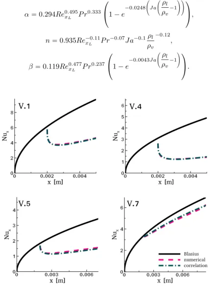
2.3.2 Correlations on the Nusselt number . . . 33
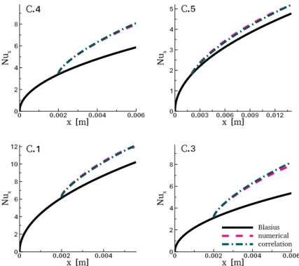
2.3.3 Validation of the proposed correlations . . . 36
2.3.4 Asymptotic cases . . . 36
2.3.5 Normal velocity and thermal flux interdependency . . . 39
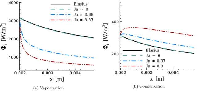
2.3.6 Integrated heat flux . . . 39
2.3.7 Viscous friction . . . 41
2.4 Conclusion . . . 44
3 Turbulent boundary layer modeling 47 3.1 Introduction to the physics of wall turbulence . . . 49
3.1.1 Characteristic quantities of wall turbulent flow . . . 50
3.1.2 Turbulent boundary layer equations . . . 51
3.1.3 Reynolds stress tensor and the turbulent kinetic energy balance equation . 53
3.1.4 Mean velocity profile . . . 55
3.2 Review of the numerical simulation methods for turbulent flows . . . 57
3.2.1 Generation of inflow boundary conditions for a turbulent flow . . . 57
3.2.2 Selection criteria . . . 64
3.2.3 Generation of inflow boundary conditions for a turbulent boundary layer with heat transfer . . . 66
3.3 Synthetic Eddy Method (SEM) . . . 68
3.3.1 Basic equations of the SEM . . . 68
3.3.2 Preliminary validation of the SEM . . . 69
3.3.3 Configuration of the SEM for a turbulent boundary layer flow . . . 75
3.3.4 Extension of the SEM for a thermal boundary layer . . . 75
3.4 Inlet plane statistics obtained using the SEM . . . 76
3.4.1 Computational configuration . . . 76
3.4.2 Computational constraints . . . 77
3.4.3 Mesh grid and number of eddies influence onto the inlet statistics . . . 78
3.5 Numerical simulation of a turbulent boundary layer flow with heat transfer at Reθ“ 1100 . . . 82
3.5.1 Computational configuration . . . 82
3.5.2 Results . . . 83
3.6 Conclusions . . . 91
4 Interaction between liquid/vapor phase change and a spatially developing tur-bulent boundary layer flow 95 4.1 Introduction . . . 96
4.2 Computational configuration . . . 96
4.2.1 Treatment of the liquid/vapor phase change . . . 97
4.2.2 Validation of the proposed treatment of liquid/vapor phase change on the 2D laminar configuration . . . 98
4.3 Influence of the spatial extension in the streamwise direction onto the development of the turbulent boundary layer flow . . . 99
4.4 Results . . . 101
4.4.1 Qualitative study . . . 103
4.4.2 Quantitative study . . . 105
4.4.3 Nusselt number . . . 108
4.5 Conclusions and perspectives . . . 110
5 Interaction between liquid/vapor phase change and natural convection induced flow 113 5.1 Introduction . . . 114
5.2 Short overview on the numerical simulation of natural convection . . . 115
5.3 Numerical method for the simulation of low Mach number liquid/vapor flows . . . 116
5.3.1 Gas phase treated using the low-Mach number approximation . . . 116
5.3.2 Liquid phase treated using the low-Mach number approximation . . . 118
5.4 Validation test case . . . 118
5.5 Present work . . . 120
5.5.2 Wall conduction . . . 121 5.5.3 Preliminary results . . . 122 5.6 Conclusions and perspectives . . . 128
Conclusions and future directions 129
Appendix A Parametric study fo the laminar boundary layer 133 Appendix B Inlet plane statistics obtained using the SEM 138 B.1 Time convergence . . . 138 B.2 Modified SEM . . . 138 B.3 Comparaison on the obtained inlet statistics when different boundary conditions are
used . . . 138 Appendix C Turbulent boundary layer interaction with liquid/vapor phase change142 C.1 Time convergence . . . 142 C.2 Mesh grid influence . . . 142 Appendix D Research paper: On the influence of liquid/vapor phase change onto
the Nusselt number of a laminar superheated or subcooled vapor flow 145
Industrial context
The interaction between liquid/vapor phase change and an external flow plays an important role in various fields, such as in combustion applications, weather forecasting, heat exchangers or climate modeling. The study of such a phenomena represents, first of all, a theoretical and a scientific challenge. In addition, having a better understanding of the heat and mass transfers in such a configuration could allow a performance enhancement of numerous industrial devices.
In particular, the space sector is also concerned by this field in the case of a space launcher, and this, at different steps of the mission: launching phase, ballistic flight, orbit insertion, etc.
When launching a space rocket, a part of the embedded liquid propellant (ergol) is stored in cryogenic tanks for later employement, during space manoeuvres. However, the tanks are heated through solar radiation or engines thermal dissipation. Thus, the temperature of the tank wall is highly increased. The thermal gradient between the tank wall and the contained ergol generates liquid/vapor phase change. The presence of vapor increases the internal pressure of the tank, which, in the context of the tank pressurization, leads to fuel loss. Hence, a better understanding of the liquid/vapor phase change and its interaction with the induced flows in a cryogenic tank could allow an optimisation of the embarked liquid propellant.
It is in this industrial context that the present thesis is placed. The tool used to tackle this subject is direct numerical simulation (DNS). The DNS of the entire cryogenic tank, together with all the involved physical phenomena, is, of course, out of reach, for computational costs and complexity reasons. Industrial codes are already employed for the simulation of a cryogenic tank. However, the lack of a good resolution of the interface between liquid and vapor phases prevents an accurate computation of the mass and heat transfers induced by the phase change. The intended concept would be to determine, by means of DNS, behaviour laws for the thermal and mass transfers at the liquid/vapor interface, laws that will further be used to model the interface in the industrial codes.
The main objective of this thesis has therefore been to simulate configurations describing the interaction between the liquid/vapor phase change and the internal cryogenic tank flows, with the focus on the interface thermal transfer.
Numerical approach
The choice of the computational configuration was not straightforward. Depending on the various phases of the flight mission, the involved physical phenomena differ. These changes are driven, inter alia, by the presence or the absence of gravitational accelerations. These two configurations are described in what follows, begining with the microgravity regime.
superheated vapor
subcooled liquid
pressurization
solar radiation
Figure 1: Schematics of the cryogenic tank subjected to microgravity, during the presurrization of the subcooled liquid by a superheated vapor. The tank wall is heated through solar radiation. The red rectangle represents the zone where the DNS will be used to characterize the vapor flow and the phase change at the liquid/vapor interface.
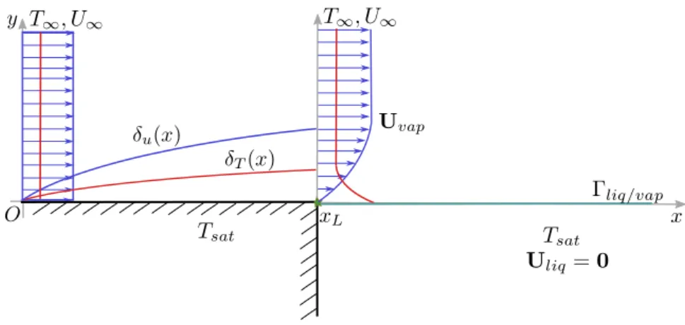
In space, the ergol is drained from the cryogenic tank for different manoeuvres, such as the orbit insertion or change of position. In order to maintain a certain internal pressure, the subcooled liquid is pressurized by a superheated vapor or a non-condensable gas. Considering the absence of the gravitational field, this procedure also allows to pack the liquid propellant. A schematic of this configuration is showed in figure 1. The approach employed for the simulation of such a configuration in microgravity has been to consider only a narrow zone at the liquid/vapor interface where the vapor flow can be modeled by a boundary layer flow, schematized by a red rectangle in figure 1. The liquid phase is considered to be static and at saturation temperature while a thermal gradient is imposed in the vapor phase. Both laminar and turbulent regimes are investigated. The influence of the liquid/vapor phase change on the interface thermal flux evolution and on the development of the laminar or turbulent boundary layer are studied.
On the other hand, during the launching phase, the tank is subjected to high gravitational accelerations, while heated through engines thermal diffusion. Residual gravitational accelerations can also be generated in space, when the engines are reignited for the orbit insertion of the satellite. Figure 2 illustrates a schematic of the tank under these conditions. The gravitational field induces a thermal stratification in the liquid, while phase change occurs at the liquid/vapor interface. Convective motions are generated in the liquid phase, that will interact with the liquid/vapor phase change. Note that, for this industrial application, the regime is turbulent, with values of the Grashof number of order „ 1010. The DNS of turbulent natural convection is complex
and have a high computational cost. For these reasons, the numerical approach is to consider a 2D laminar configuration of a two phase flow containing a subcooled liquid and a vapor flow initially at saturation temperature. The solar radiation heat flux is modeled by imposing a wall conduction heat flux. Laminar natural convection flow, defined by a Grashof number of „ 106,
is induced in the liquid. Even if, in terms of flow regime, the studied configuration is different from the industrial configuration, this can be seen as a first step before pursuing with more precise studies. Additionally, the preliminary results obtained with the 2D configuration will allow a better understanding of the physical phenomena involved when natural convection mouvements interact with liquid/vapor phase change.
superheated vapor
subcooled liquid
solar radiation
engines thermal diffusion convective motions
Figure 2: Schematics of the cryogenic tank subjected to gravitational accelerations, containing a subcooled liquid pressurized by a superheated vapor. The tank wall is heated through solar radi-ation or/and engines thermal diffusion. The red rectangle represents the numerical configurradi-ation studied in the present thesis.
Before describing the outline of the thesis, it is important to stress that, often, the studied con-figurations, both by numerical or experimental approaches, differ from the very complex industrial problems. However, this does not diminish, in any way, their scientific and theoretical importance. Moreover, the interlock of decoupled physical phenomena or of simplistic configurations, allows in the end the comprenhension of more complex industrial processus.
Outline of the Thesis
The work carried out during the course of this thesis is presented as follows.
Chapter 1 is dedicated to the description of the in house code, DIVA, used for the direct nu-merical simulation of the above described configurations. The nunu-merical methods implemented to solve the physical model translating the behaviour of two-phase flows with phase change are pre-sented: the Level-Set method for the interface capture, the projection method for the Navier-Stokes equations, and the Ghost Fluid Thermal Solver for Boiling used to solve the energy conservation equation.
In chapter 2, we present a numerical study to characterize the interaction between a superheated or subcooled external laminar vapor flow shearing a static and plane liquid pool at saturation temperature. Our purpose was to find, for this configuration, correlations on the Nusselt number accounting for the modification of the local thermal gradient on the interface due to the vaporization or condensation induced flow. As the local structure of the flow is also modified in the vicinity of the liquid-vapor interface, our study includes an analysis on the interfacial viscous friction when phase change occurs.
In practical applications, most flows which occur are turbulent. Therefore, the subsequent topic of our work concerns the interaction between a turbulent boundary layer flow and the velocity field induced by liquid/vapor phase change. To this extent, the spatial evolution of a turbulent boundary layer flow on a flat plate has first to be simulated. This work is described in chapter 3. After a thorough overview of the existing numerical methods for the generation of turbulent fluctuations, the chosen method is described and validated. Next, the results obtained are presented
and discussed. A particular attention is also paid to the computational constraints related to the simulation of turbulent boundary layer flows.
In chapter 4, we investigate the interaction between a spatially developing turbulent bound-ary layer flow and a normal velocity field induced by liquid/vapor phase change. This is first conducted qualitatively, by analysing the normal velocity field, the vorticity magnitude field and the isosurfaces of the Q criterion. Next, a study on the influence of the phase change onto the turbulent quantities is presented. Several Jakob numbers are studied and a preliminary physical analysis is proposed for the obtained profiles. Additionally, we take interest on the impact of the phase change onto the Nusselt number evolution. This is given in the continuity of the work on the laminar regime where correlations on the Nusselt number are proposed.
In chapter 5, the focus is on the liquid phase where natural convection motions develop and interact with the liquid/vapor phase change. A 2D computational configuration is considered, where the density variations in the liquid phase are treated using the low-Mach approximation while the vapor phase is incompressible. The vapor is initially at saturation temperature and the liquid is subcooled. Wall conduction is considered for the boundary conditions on the vertical walls. A natural convection flow is induced in the liquid and its interaction with the liquid/vapor phase change is investigated. Different values of the Grashof number are studied and a discussion on its influence on the thermal flux is given. The study is in progress and opens to many perspectives.
Numerical methods
Contents
1.1 Introduction . . . 6
1.2 General background on two-phase flows numerical simulation . . . 6
1.2.1 Interface localization . . . 6
1.2.2 Modeling two-phase flows . . . 9
1.2.3 Ghost Fluid method . . . 12
1.3 Numerical model for two-phase flows - DIVA code . . . 14
1.3.1 Level-Set discretization . . . 15
1.3.2 Computation of the intermediate velocity . . . 16
1.3.3 Pressure field resolution . . . 18
1.3.4 Extension methodology to impose the free divergence onto the velocity field . . . 19
1.3.5 Ghost Fluid Thermal Solver for Boiling . . . 20
1.3.6 Extrapolation techniques for a scalar field . . . 21
1.3.7 Temporal discretization . . . 22
1.4 Conclusion . . . 23
The numerical study of the interaction between an external flow and the liquid/vapor phase change has been conducted using the in house code, DIVA. The code DIVA, that states for Interfacial Dynamics for Atomization and Vaporization, allows for direct nu-merical simulation of two-phase flows with phase change. In this chapter, this nunu-merical tool is described.
1.1
Introduction
In this chapter we try to provide a comprehensive overview of two-phase flows numerical simula-tion. To this extent, the first section tackles the three major aspects of two-phase flows simulation, i.e. the interface localization, the formalism to solve the corresponding physical equations and the treatment of the interface discontinuities. In the second part of this chapter, the code DIVA is described. First, the methods for interface localization are described, then the physical equations translating the behaviour of two-phase flows with phase change are presented. Finally, the numer-ical methods implemented to solve this physnumer-ical model are expounded: the Level-Set method for the interface capture, the projection method for the Navier-Stokes equations, and the Ghost Fluid Thermal Solver for Boiling used to solve the energy conservation equation.
1.2
General background on two-phase flows numerical
simu-lation
Two-phase flows simulations entail the use of a numerical model allowing above all to locate the interface between the two phases. Additionally, algorithms for solving the physical equations as well as treating the discontinuities across the interface are needed. A general background on these aspects is given in what follows.
1.2.1
Interface localization
The notion of interface is inherent in the context of two-phase flows. A large amount of literature relevant to interfaces exists. For example, in the classical work of Germain [25], the interface separating two immiscible fluids is defined as a geometric surface at which a discontinuity in properties occurs. Jump conditions through the interface are derived from the classical balance laws for mass, momentum and energy.
To numerically simulate two-phase flows, each phase distribution as well as the interface position have to be known at all times. Two approaches describing the time evolution of an interface can be distinguished: the Lagrangian or Tracking methods and the Eulerian or Interface-Capturing methods.
The Lagrangian approach implies the use of markers or particles without mass whereas in the Eulerian approach a scalar field defining the presence of a fluid or of the interface is used. Both the markers and the scalar field are convected by the local velocity field throughout the entire domain. In what follows, a survey of the existing methods is given.
1.2.1.1 Lagrangian methods
Numerous Lagrangian methods exist. One of the first is the Mark and Cell method (MAC) proposed by Harlow and Welch [30] where lagrangian markers are placed only in the region of one of the phases. The major drawback of this method is the large number of markers needed to correctly model the fluids distribution (figure 1.1a). To adress this, Daly [17] proposes a slighthly different method where markers are dispersed only on the interface. Nevertheless, to obtain an accurate position of the interface, the distance between two consecutive points has to remain small enough and regular. This leads us to the Front Tracking methods, introduced by Glimm et al. [14, 28]. The markers are regularly distributed along the interface, forming segments in 2D and triangles in 3D (figure 1.1b). The most common version of this method was proposed by Unverdi and
Tryggvason [105]. This type of approach is not the most appropriate to the simulation of the interaction between several interfaces, in the case of rupture or coalescence.
Markers fluid 1 fluid 2 Interface (a) MAC Markers fluid 1 Interface fluid 2 (b) Front Tracking
Figure 1.1: Illustration of Lagrangian methods.
The Boundary Fitted methods, another Lagrangian approach, involves that the mesh grid is adapted to the interface shape. This allows modeling the interface jump conditions as classical boundary conditions. Since the mesh grid is aligned with the interface, the accuracy is greatly improved. Nevertheless, the main drawback is that the mesh grid is evolving with the interface and has to be reconstructed at each time step. The computation time is therefore greatly increased. This type of approach has particularly be used for bubble rising simulations [18, 89].
1.2.1.2 Eulerian methods
The Eulerian methods are based on the definition of a particular scalar field within the global fixed mesh grid. This scalar field is advected by the local velocity at each time iteration. It allows in this way to compute the localization of the two fluids as well as the interface position. The Eulerian methods can be divided into two major categories: the Volume of Fluid (VOF) and the Level-Set methods. fluid 1 fluid 2 0 0.75 0.8 0.05 1 1 0 0 0 0 0 0 0.3 0 0.23 0.9 0.55 0.7 1 1 (a) VOF fluid 1 fluid 2 0 0.75 0.8 0.05 1 1 0 0 0 0 0 0 0 0 0.7 1 1 0.3 0.23 0.7 0.55 0.75 0.8 1 1 1 1 0.9 fluid 2 (b) VOF SLIC fluid 1 0 0 0 0 0 fluid 2 0.75 0.8 0.05 1 1 0 0.3 0 0.9 0.55 1 1 0 0.23 0.7 (c) VOF SPLIC
Figure 1.2: Different VOF methods: initial form and C values (a), interface reconstruction with the SLIC (b) and SPLIC (c) algorithms.
The VOF method, proposed by Hirt and Nichols [33], uses a scalar function C characterizing the volume fraction of one of the two fluids present in the cell grid (figure 1.2a). Thus, if the fluid occupies the entire cell, C “ 1 whereas if the cell is filled only with the second fluid, C “ 0. It
follows naturally that the cell crossed by the interface contains the two fluids and 0 ă C ă 1. The scalar field C is advected by the local velocity field u,
BC
Bt ` u ¨ ∇C “ 0. (1.1)
The scalar field C is constant in each fluid region and varies greatly across the interface. Con-sequently, a very accurate discretization is needed for the computation of the convective term from equation (1.1). The advantage of the VOF method is its mass conservation in time. Nonetheless, the computation of the geometric properties, such as the interface curvature and the normal vec-tor, is not straightforward. This is caused by the fact that the precise location of the interface is unknown. Indeed, a reconstruction algorithm is necessary at each time step in order to reconstitute the interface using the discrete values of the function C. Noh and Woodward [68] introduced the first reconstruction algorithm, the SLIC (Simple Line Interface Calculation) where the interface is formed by line segments aligned with the mesh principal directions (figure 1.2b). An improvement of the SLIC method is proposed by Youngs [110] where the interface is now approximated by a line segment non-aligned with the mesh (figure 1.2c). This method, named PLIC (Piecewise Line Interface Calculation) uses the values of the field C at the grid neighbouring points to calculate the line segment orientation in the corresponding cell. Since the introduction of the VOF methods, nu-merous modifications have been done in order to improve the accuracy of the temporal evolution of the interface, as well as the calculation of its geometric properties (see [7, 9, 29, 51, 78, 80, 85, 91]). The second category of Eulerian approaches is represented by the Level-Set method, introduced by Osher and Sethian [69]. A scalar field φ corresponding to the signed distance to the interface is defined in the entire computational domain Ω. The latter is decomposed into two regions Ω` and
Ω´, representatives of the two respective fluids,
Ω`“ tx P Ω | φpxq ą 0u , (1.2)
Ω´“ tx P Ω | φpxq ă 0u , (1.3) whereas the interface is characterised by the level 0 of the φ function
Γ“ tx P Ω | φpxq “ 0u . (1.4) It is therefore possible to define, by extension, a level lines ensemble Γk in the computational
domain Ω, located at a distance |dk| from the interface (figure 1.3),
Γk“ tx P Ω | φpxq “ |dk|u . (1.5)
Figure 1.3: Level set function corresponding to a circular interface.
As a result, the computation of the physical properties of each fluid, such as the density ρ and the dynamic viscosity µ, is direct.
The temporal evolution of the interface is done by the use of the following advection equation, Bφ
Bt ` u ¨ ∇φ “ 0. (1.6)
This type of equation is known to develop discontinuous solutions even if the initial field is contin-uous. Hence, a robust scheme has to be employed to deal with possible singularities.
Compared to others Interface-Capturing methods, the Level-Set method allows a simple and accurate computation of the interface geometric properties. The normal vector to the interface is calculated with
n“ ∇φ
||∇φ||, (1.7)
and the interface curvature can be deduced with κ“ ∇ ¨ n “ ∇ ¨ ˆ ∇ φ ||∇φ|| ˙ . (1.8)
On the other hand, this method has two major drawbacks. Firstly, the existence of high shearing or streching zones in the velocity field can considerably spread or tighten the level lines, degrading therefore the geometric properties of the Level Set function. Indeed, the advection equation (1.6) is solved for all the level lignes Γk, whereas the displacement speed is known only
for the interface, since their definition is purely mathematical. Sussman et al. [99] proposed to solve a redistancing equation which forces φ to be a signed distance to the interface for every time step, without changing the zero level curve location. To this extent, the following equation
Bd
Bτ “ signpφq p1 ´ |∇d|q (1.9) is iterated for a few fictitious time steps τ . The interface position is conserved by imposing the initial condition d px, t, τ “ 0q “ φpx, tq.
Secondly, the numerical dissipation of the advection equation (1.6) discretization can cause mass losses. Additionally, during the redistancing step (1.9), the interface position can be slightly changed and induces a gain or loss in mass. Nevertheless, the interface perturbation remains low if the mesh grid is refined enough. As for the numerical dissipation of the advection equation, this can be adressed, inter alia, by the use of a more accurate discretization scheme.
1.2.2
Modeling two-phase flows
In this section, we present the physical equations and the numerical approach used in the con-figuration of two-phase flows. All thermodynamic properties are considered to be constant. The specific case of variable density will be discussed later.
1.2.2.1 Physical equations
An incompressible one-phase fluid flow, in a domain Ω, is described by the Navier-Stokes equations,
∇¨ u “ 0, (1.10) ρ ˆ Bu Bt ` pu ¨ ∇q u ˙ “ ´∇p ` ∇ ¨´2µ ¯D¯¯` ρg, (1.11) with t the time, ρ and µ the fluid density and dynamic viscosity, respectively, u “ pu, v, wq the velocity field, p the pressure field, g the gravitational acceleration and ¯¯D the strain tensor defined by ¯ ¯ D“∇u` ∇ Tu 2 . (1.12)
The thermal field is described by a simplified energy conservation equation, formulated using the enthalpy primitive variable
ρCp ˆ BT Bt ` pu ¨ ∇q T ˙ “ ∇ ¨ pk∇T q , (1.13) where T is the thermal field, Cp is the specific heat at constant pressure and k is the thermal
conductivity.
We now consider that the domain Ω contains two regions Ω` and Ω´, each corresponding to
a different phase. As a result, the two fluids physical properties are employed respective to each fluid as: (ρ`, µ`, k`, C`
p) and (ρ´, µ´, k´, Cp´).
The liquid and the vapor phases are separated by an interface Γ, across which phase change can occur (i.e. the liquid vaporizes into vapor or the vapor condenses into the liquid). Across the interface, the continuity of the mass flux, the momentum and enthalpy balances have to be satisfied.
The interface mass flux, 9m is obtained by applying the mass conservation (1.10) across the interface,
9
m“ ρlpVl´ VΓq ¨ n “ ρvpVv´ VΓq ¨ n, (1.14)
where the interface velocity is denoted by VΓ and n is the local unit vector pointing towards the
liquid phase. The subscripts l and v are used to refer to the liquid and vapor phases, respectively. The jump on the velocity field across the interface can therefore be written as:
rVsΓ“ 9m „ 1 ρ Γ n, (1.15)
where the operator r¨sΓaccounts for the jump across the interface and it is defined by: rfsΓ“ fv´fl.
The momentum balance at the interface is imposed by integrating the momentum equation (1.11) across the interface and by including the effects of the surface tension,
„ p´ 2µBVn Bn ` ρpV ¨ n ´ VΓ¨ nq 2 Γ “ σκ, (1.16)
which, by using equation (1.15), is rewritten as
rpsΓ “ σκ ` 2 „ µBVn Bn Γ ´ 9m2 „ 1 ρ Γ , (1.17)
where σ is the surface tension, κ is the interface curvature and BVn
Bn is the normal derivative of the
normal velocity component. The first term of the right hand side of this equation is the capillary pressure from the Laplace-Young law, the second term accounts for the discontinuity of the normal viscous stress, and the last term is usually referred as the recoil pressure.
According to the second law of thermodynamics and assuming that the local equilibrium hypothesis is still valid, the interface temperature is imposed to be the saturation temperature Tl“ Tv“ Tsat. Integrating equation (1.13) across the interface yields
rρh pVl´ VΓq ¨ nsΓ “ r´k∇T ¨ nsΓ, (1.18)
where h defines the enthalpy. It is assumed that h depends only on the temperature. By using equation (1.15), the jump condition for the energy conservation writes
9
mLv “ r´k∇T ¨ nsΓ, (1.19)
The physical model that has to be solved in two-phase flow simulations is represented by the Navier-Stokes equations (1.10)-(1.11), the energy conservation equation (1.13), along with the interface jump conditions (1.15), (1.17), (1.19). Thus, in comparison with single phase flows, the resolution of two-phase flows presents two issues: the treatment of the discontinuities across the interface and modeling of the jump conditions. The two points in question will be further discussed. There are two types of formulations for the Navier-Stokes equations, when incompressible two-phase flows are concerned: the Whole-Domain formulation [11, 91] and the Jump-Condition for-mulation. As their names suggest it, the Whole-Domain formulation implies the resolution of the physical equations in all the domain whereas in the Jump-Condition formulation, the physical equations are solved in each phase and jump conditions are imposed at the interface.
Concerning the treatment of the discontinuities across the interface, two approaches can be distinguished:
- the Continuum Surface Force formalism, where the discontinuities are smoothed over 2-3 grid cells with the aid of the Heaviside distribution HΓ; the inconvenient of this approach is
the development of parasitic currents leading to numerical instabilities.
- the Sharp Interface methods, where the discontinuities are treated as jump conditions, pre-venting the interface thickening and reducing parasitic currents magnitude.
1.2.2.2 Projection method for solving Navier-Stokes equations
The temporal discretization of the Navier-Stokes equations (1.10)-(1.11), with velocity and pressure fields unknown at the time step tn`1, yields
∇¨ un`1“ 0, (1.20) ρ ˆun`1´ un ∆t ` pu n¨ ∇q un ˙ “ ´∇pn`1` ∇ ¨´2µ ¯D¯n¯` ρg. (1.21)
The obtained equations are numerically solved by the use of the projection method introduced by Chorin [15] for single phase flows. The latter is based on the Hodge decomposition of any vector field into the sum of an irrotational (curl-free) vector field and a solenoidal (divergence-free) vector field. This method allows to decouple the resolution of the Navier-Stokes equations into the velocity field u resolution and the pressure field p resolution.
For two-phase flows, the use of this approach is not straightforward. Some modifications have to be done depending upon the chosen formulation. The method is further described for a Jump-Condition formalism, since it is implemented in the code DIVA.
The first step, also called the prediction step, is based on the calculation of an intermediate velocity u˚ as u˚“ un´ ∆t ¨ ˝pun¨ ∇q un´ ∇¨ ´ 2µ ¯D¯n¯ ρ ´ g ˛ ‚. (1.22)
Replacing this expression into equation (1.21) yields
u˚“ un`1` ∆t∇p
n`1
ρ , (1.23)
and in this way we obtain the decomposition of the velocity field u˚ into a free divergence
enforcing the free divergence on this decomposition, the Poisson equation on the pressure is ob-tained ∇¨ ˆ∇ pn`1 ρ ˙ “ ∇¨ u ˚ ∆t . (1.24)
with at the interface the jump condition on the pressure (1.17). It will be demonstrated in section 1.2.3 that adding a source term in the right hand side of the Poisson equation is equivalent with imposing a jump condition,
∇¨ ˆ∇ pn`1 ρ ˙ “∇¨ u ˚ ∆t ` ∇ ¨ ˆ σκnδΓ ρ ˙ . (1.25)
Finally, the velocity field un`1 can be directly deduced from the Hodge decomposition, as
un`1“ u˚´∆t ρ
`
∇pn`1´ σκnδΓ˘. (1.26) where δΓ is the Dirac delta function, non-zero only at the interface.
1.2.3
Ghost Fluid method
The Ghost Fluid method allows to adress the jump conditions at the interface for a system of partial differential equations discretized on a cartesian grid. This approach have been introduced by Fedkiw et al. [23] to compute non-viscous fluid flows with discontinuities at the interface. Later, it has been extended by Kang et al. to incompressible viscous two-phase flows with surface tension and gravity [43].
This approach is based on the accurate subgrid localization of the region where the discontinuity occurs thanks to the interface capture. The differential schemes are modified in order to avoid the presence of discontinuities related to the jump across the interface. For a better understanding of this procedure, figure 1.4 shows a 1D exemple. In each fluid region (purple for x ă xΓ or blue for
xą xΓ) the real values of the function f are known. They are extended by continuity at a certain
number of grid points in the region across the interface by using the known value of the jump. This so called ghost values are used in the derivation schemes to ensure the continuity while preserving the f jump value at the interface.
i-1
x
x
ix
i+1 i+2x
f
[f]
-Figure 1.4: Schematics of the jump variable for Ghost Fluid method: real values ( ) and ghost values ( ).
The spatial discretization of the 1D Poisson equation, proposed in [61], B Bx ˆ βBf Bx ˙ “ Rhs, (1.27)
using a centered scheme of second order, is expressed as βi`1{2fi`1´ fi ∆x ´ βi´1{2 fi´ fi´1 ∆x ∆x “ Rhs|i, (1.28) where Rhsstates for right hand side of the Poisson equation.
Further, the three possible configurations, the jump on the function rfsΓ “ a pxΓq (fig. 1.4),
the jump on the flux ”βBfBxı
Γ “ b pxΓq and the jump on the diffusion coefficient rβsΓ ‰ 0 are
described. The three conditions can be combined and the extension to 2D or 3D configurations is straightforward.
1.2.3.1 Variable jump
We first consider the variable jump rfsΓ “ a pxΓq at the interface Γ situated between the grid
points xi and xi`1, as in figure 1.4. The spatial discretization of equation (1.27), with respect to
each fluid region, yields
βi`1{2f ` i`1´ fi´ ∆x ´ βi´1{2 fi´´ fi´1´ ∆x ∆x “ Rhs|i. (1.29) We recall that the symbols ` and ´ state for the fluid region for which the value is considered: Ω` or Ω´. The discretization of the first derivative contains a jump on the function f since the
cell rxi, xi`1s is crossed by the interface. To avoid this, the function fi`1` is replaced by its ghost
value fG,´
i`1 defined as
fi`1G,´ “ fi`1` ´ rfsΓ“ fi`1` ´ a pxΓq . (1.30)
The discretization of the Poisson equation, without mixing terms from both fluid regions, becomes βi`1{2f G,´ i`1 ´ fi´ ∆x ´ βi´1{2 fi´´ fi´1´ ∆x ∆x “ Rhs|i. (1.31) and, by the use of the ghost value definition (1.30),
βi`1{2 ` fi`1` ´ a pxΓq ˘ ´ f´ i ∆x ´ βi´1{2 fi´´ f´ i´1 ∆x ∆x “ Rhs|i, (1.32) or βi`1{2 fi`1` ´ fi´ ∆x ´ βi´1{2 fi´´ fi´1´ ∆x ∆x “ Rhs|i` βi`1{2 apxΓq ∆x2 . (1.33)
The original discretization of the Poisson equation is obtained with an additional source term allowing to account for the jump condition between xiand xi`1.
In the same way, the discretization at the grid point xi`1 accounting for the jump condition,
writes βi`3{2 fi`2` ´ fi`1` ∆x ´ βi`1{2 fi`1` ´ fi´ ∆x ∆x “ Rhs|i`1´ βi`1{2 apxΓq ∆x2 . (1.34) 1.2.3.2 Flux jump
We now consider the configuration where a jump on the flux has to be imposed, defined as”βBfBxı
Γ “
bpxΓq. The spatial discretization of the Poisson equation (1.27), at a grid point xi gives:
ˆ βi`1{2 fi`1´ fi ∆x ˙` ´ ˆ βi´1{2 fi´ fi´1 ∆x ˙´ ∆x “ Rhs|i, (1.35)
with the symbols ` and ´ corresponding to the regions where the flux is computed. The derivative between the grid points xi´1{2 and xi`1{2is not continous as a result of the jump at the interface.
The ghost values of the flux are defined, by continuity, on the grid points across the interface ˆ βi`1{2 fi`1´ fi ∆x ˙G,´ “ ˆ βi`1{2 fi`1´ fi ∆x ˙` ´ „ βBf Bx Γ “ ˆ βi`1{2 fi`1´ fi ∆x ˙` ´ bpxΓq. (1.36)
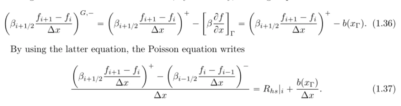
By using the latter equation, the Poisson equation writes ˆ βi`1{2 fi`1´ fi ∆x ˙` ´ ˆ βi´1{2 fi´ fi´1 ∆x ˙´ ∆x “ Rhs|i` bpxΓq ∆x . (1.37) 1.2.3.3 Diffusion coefficient jump
The third possible configuration presumes a discontinuity on the diffusion coefficient. Considering the 1D example from figure 1.4, the discretization of the Poisson equation (1.27) includes the values βi´1{2 and βi`1{2. As it can be observed in fig. 1.5, the value βi´1{2“ β´, as both the grid
points xi and xi´1 are located in Ω´. To calculate βi`1{2, we use the continuity of the flux at the
interface, that writes
βi`1{2fi`1´ fi ∆x “ β ´ fΓ´ fi p1 ´ θq∆x“ β `fi`1´ fΓ θ∆x , (1.38)
where fΓ represents the value of f at the interface.
Figure 1.5: Interface-grid intersection and jump on the diffusion coefficient for Ghost Fluid method.
As a result, from the latter equation, the value of fΓ is expressed as
fΓ“
β´fiθ` β`fi`1p1 ´ θq
β´θ` β`p1 ´ θq , (1.39)
where θ “ |φi`1|
|φi| ` |φi`1|, φ being the Level-Set function known at each grid point.
By replacing this expression in (1.38), the value of the diffusion coefficient yields
βi`1{2“ β
´β`
β´θ` β`p1 ´ θq. (1.40)
The jump on the diffusion coefficient does not imply the addition of a source term in the right hand side of the equation. Nevertheless, the coefficients of the linear system matrix are modified.
1.3
Numerical model for two-phase flows - DIVA code
In this section, the numerical solver implemented in the code DIVA is detailed. It allows the computation of incompressible two-phase flows with a jump condition on the normal velocity at the interface. Nguyen et al. [67] were the first to use it to capture flame discontinuities. Kang
et al. [43] and Sussman et al. [100] extended it for the simulation of incompressible two phase flows without phase change. The approach Ghost Fluid allowing to account for the velocity jump at the interface, when phase change occurs, was employed in several papers. Gibou et al. [26] and Tanguy et al. [102] applied it for boiling simulation. For an accurate simulation of drops evaporation, Tanguy et al. [101] propose an improvement of the method in order to properly impose the free divergence condition at the interface for the liquid velocity field.
The interface separating the two-phases is located using the Level-Set method, that allows splitting the computational domain Ω into two regions corresponding to each phase: Ω` for the
liquid phase and Ω´ for the vapor phase (see details on the Level-Set method in section 1.2.1.2).
A global scalar field is defined for each physical property, such as
ρpxq “ #
ρ` if x P Ω`
ρ´ if x P Ω´ . (1.41) The same goes for the dynamic viscosity µ, the specific heat Cp and the thermal conductivity k.
Their discontinuity across the interface is treated using a Sharp-Interface approach.
The physical model is represented by the mass (1.10), momentum (1.11) and energy (1.13) conservation equations along with the corresponding interface jump conditions (1.15), (1.17) and (1.19). Its resolution is done in the framework of Jump-Condition formulation, with the Ghost-Fluid Method for the jump conditions treatment.
In what follows, the various steps of the solver algorithm, as well as the corresponding spatial discretizations, are given. For the sake of simplification, the 2D configuration is considered, but the extension to 3D is straightforward.
In the context of this thesis, we use a cartesian mesh grid of MAC (Marker and Cell) type, represented in figure 1.6. The formalism of this kind of mesh grid is that the different variables are not computed on the same grid. The scalar fields (pressure, Level-Set function, ...) are defined at the center of the cell grid while the velocity components are staggered at the cell face centers. The spatial discretization follows from a finite-volume approach.
Figure 1.6: Variables definition on the mesh grid.
The different convective terms are discretized with a WENO-Z scheme [10]. The resolution of the linear systems obtained for the pressure and the thermal fields is carried out with the Black Box MultiGrid method (BBMG) [22, 63]. The details on the implementation of this solver in the DIVA code can be found in [56].
1.3.1
Level-Set discretization
The level-set function φpi, jq is defined at the cell center. At each temporal iteration, the interface is convected using (1.6) while considering the velocity field un from the previous time step tn. The
resolution is explicit in time, writing
φn`1“ φn´ ∆t pun¨ ∇q φn, (1.42) with ∆t the time step.
Once the level-set function is computed at the time tn`1, the redistancing algorithm is applied
to adjust the distance between consecutive levels. An explicit scheme is used on the fictitious time τ and the absolute value of the distance function d is obtained with the WENO-Z scheme,
#
dm`1 “ dm´ ∆τsign`φn`1˘p1 ´ ||∇dm||q
dm“0 “ φn`1 , (1.43)
where ∆τ is the fictitious time step. A few temporal iterations are performed to obtain the algorithm convergence. Thereafter, the distance function replaces the level-set field φn`1. The
fluids physical properties are updated using the novel value of the level-set function, as
ρn`1pφn`1q “ ρ´` H Γpφn`1q ` ρ`´ ρ´˘, (1.44) µn`1pφn`1q “ µ´` HΓpφn`1q ` µ`´ µ´˘, (1.45) with the Heaviside distribution expressed as
HΓ ` Φn`1˘“ # 1 if φn`1ą 0 0 if φn`1ă 0 . (1.46)
Next, the resolution of the Navier-Stokes equations, performed using the projection method, is detailed. The following sections are organized as follows: first the general algorithm is given for two-phase flows, and next, the extensions required to deal with phase change are presented.
1.3.2
Computation of the intermediate velocity
The first step in the projection method is the computation of the intermediate velocity field u˚.
In the code DIVA, the viscous term has an implicit treatment,
ρn`1u˚´ ∆t∇ ¨´2µn`1D¯¯˚¯“ ρn`1pun´ ∆t ppun¨ ∇q un´ gqq . (1.47) First, the terms of the right-hand side of equation (1.47) are computed,
Rhs“ ρn`1pun´ ∆t ppun¨ ∇q un´ gqq . (1.48)
Next, the resolution of (1.47) leads to a large linear system where the two velocity components are coupled. This velocity field does not need an interface jump condition, however, the diffusion coefficient in the viscous term corresponding to the dynamic viscosity µ, is discountinuous across the interface. The formalism described in section 1.2.3.3 is therefore used.
The discretization of the viscous term is further detailed [52]. By applying the divergence operator and by omitting the exponents symbols p.qn`1 and p.q˚, we obtain
∇¨ ´ 2µ ¯D¯¯“ ¨ ˚ ˚ ˚ ˝ B Bx ˆ 2µBu Bx ˙ ` B By ˆ µ ˆ Bu By ` Bv Bx ˙˙ B Bx ˆ µ ˆ Bu By ` Bv Bx ˙˙ ` B By ˆ 2µBv By ˙ ˛ ‹ ‹ ‹ ‚. (1.49)
The projection in the exdirection gives ∇¨´2µ ¯D¯¯¨ ex ˇ ˇi`1{2,j “ B Bx ˆ 2µBu Bx ˙ˇ ˇi`1{2,j ` B By ˆ µ ˆ Bu By ` Bv Bx ˙˙ˇ ˇi`1{2,j , (1.50)
with, by using a second order finite difference scheme,
B Bx ˆ 2µBu Bx ˙ˇ ˇi`1{2,j » 2µi`1,j ui`3{2,j´ ui`1{2,j ∆x ´ 2µi,j ui`1{2,j´ ui´1{2,j ∆x ∆x , (1.51) B By ˆ µBu By ˙ˇ ˇi`1{2,j »
µi`1{2,j`1{2ui`1{2,j`1´ ui`1{2,j
∆y ´ µi`1{2,j´1{2 ui`1{2,j´ ui`1{2,j´1 ∆y ∆y , (1.52) B By ˆ µBv Bx ˙ˇ ˇi`1{2,j » µi`1{2,j`1{2 vi`1,j`1{2´ vi,j`1{2 ∆x ´ µi`1{2,j´1{2 vi`1,j´1{2´ vi,j´1{2 ∆x ∆y . (1.53)
In the same way, the projection in the ey direction yields
∇¨ ´ 2µ ¯D¯¯¨ ey ˇ ˇi,j`1{2 “ B Bx ˆ µ ˆ Bu By ` Bv Bx ˙˙ ˇˇ ˇi,j`1 2 ` B By ˆ 2µBv By ˙ˇ ˇi,j`1{2, (1.54) with B Bx ˆ µBu By ˙ˇ ˇi,j`1{2 »
µi`1{2,j`1{2ui`1{2,j`1´ ui`1{2,j
∆y ´ µi´1{2,j`1{2 ui´1{2,j`1´ ui´1{2,j ∆y ∆x , (1.55) B Bx ˆ µBv Bx ˙ˇ ˇi,j`1{2 »µi`1{2,j`1{2 vi`1,j`1{2´ vi,j`1{2 ∆x q ´ µi´1{2,j`1{2 vi,j`1{2´ vi´1,j`1{2 ∆x ∆x , (1.56) B By ˆ 2µBv By ˙ˇ ˇi,j`1{2 » 2µi,j`1 vi,j`3{2´ vi,j`1{2 ∆y ´ 2µi,j vi,j`1{2´ vi,j´1{2 ∆y ∆y . (1.57)
In order to compute rightfully the viscous term at the intermediate time step, one must solve a coupled linear system of two matrices with 9 diagonals per velocity components as
a1i`1,ju˚i`3{2,j` a1i,ju˚i´1{2,j` b1i`1{2,j`1{2u˚i`1{2,j`1` b1i`1{2,j´1{2u˚i`1{2,j´1` αi`1{2,ju˚i`1{2,j
` c1i`1{2,j`1{2 ´ vi`1,j`1{2˚ ´ v˚ i,j`1{2 ¯ ` c1i`1{2,j´1{2 ´ vi`1,j´1{2˚ ´ v˚ i,j´1{2 ¯ “ Rhs¨ ex ˇ ˇi`1{2,j , (1.58) and
βi,j`1{2vi,j`1{2˚ ` b2i,j`1v˚i,j`3{2` b2i,jv˚i,j´1{2` a2i`1{2,j`1v˚i`1,j`1{2` a2i`1{2,j`1v˚i´1,j`1{2
` c2i`1{2,j`1{2 ´ u˚i`1{2,j`1´ u˚i`1{2,j ¯ ` c2i´1{2,j`1{2 ´ u˚i´1{2,j`1´ u˚i´1{2,j ¯ “ Rhs¨ ey ˇ ˇi,j`1{2. (1.59) The matrix coefficients are deduced from equations (1.47), (1.50) and (1.54) as
a1k,l“ ´ 2µk,l ∆x2∆t, b1k,l“ ´ µk,l ∆y2∆t, c1k;l“ ´ µk,l ∆x∆y∆t, (1.60) a2k,l“ ´ µk,l ∆x2∆t, b2k,l“ ´ 2µk,l ∆y2∆t, c2k;l“ ´ µk,l ∆x∆y∆t, (1.61)
αi`1{2,j“ ρn`1i`1{2,j´ a1i`1,j´ a1i,j´ b1i`1{2,j`1{2´ b1i`1{2,j´1{2, (1.62)
βi,j`1{2“ ρn`1
i,j`1{2´ b2i,j`1´ b2i,j´ a2i`1{2,j`1{2´ a2i´1{2,j`1{2. (1.63)
Lepilliez et al. [57] showed that, since the linear system is diagonally dominant, it can be solved efficiently with a few Gauss–Seidel iterations (ă 20 iterations for typical multiphase flow configurations). For a 3D system, a third coupled matrix has to be accounted for, resulting in a 15-diagonal matrix per velocity components.
Additional aspects when phase change occurs
When phase change occurs, the jump condition (1.15) on the mass conservation equation has to be considered. Therefore, the velocity fields correponding to the vapor and the liquid are extended as it follows u˚l “ # u˚ if φ ą 0 u˚´ 9m”1ρı Γn if φă 0 , (1.64) u˚v “ # u˚´ 9m”1 ρ ı Γn if φą 0 u˚ if φ ă 0 . (1.65)
1.3.3
Pressure field resolution
The second step of the projection method implies the resolution of the Poisson equation on the pressure (1.24). Additionally, the jump condition (1.17) has to be imposed. The formalisms described in Section 1.2.3.1 and 1.2.3.3 are therefore used. The spatial discretization of the pressure equation (1.26) is done by using the Ghost Fluid approach,
βi`1{2,j ˆ pi`1,j´ pi,j ∆x ˙ ´ βi´1{2,j ˆ pi,j´ pi´1,j ∆x ˙ ∆x (1.66) ` βi,j`1{2 ˆ pi,j`1´ pi,j ∆y ˙ ´ βi,j´1{2 ˆ pi,j´ pi,j´1 ∆y ˙
∆y “ Rhs|i,j` ηi,j, (1.67) with β “ 1{ρn`1 the diffusion coefficient,
Rhs|i,j “ u˚i`1{2,j´ u˚ i´1{2,j ∆x ` vi,j`1{2˚ ´ v˚ i,j´1{2 ∆y ∆t , (1.68)
the right hand side of the Poisson equation and ηi,j represents the source terms accounting for the
pressure jump condition.
As explained in section 1.2.3.3, when the cell grid is crossed by the interface, the diffusion coefficient β is calculated using a harmonic mean. There are two general configurations. If the interface crosses the segment rxi, xi`1s, the diffusion coefficient is computed with
βi`1{2,j “ $ ’ ’ ’ & ’ ’ ’ % β´β`
β´θE` β`p1 ´ θEq if φi,jă 0 and φi`1,j ą 0
β´β`
β`θE` β´p1 ´ θEq if φi,ją 0 and φi`1,j ă 0
where
θE “ |φi`1,j| |φi,j| ` |φi`1,j|
. (1.70)
If the interface crosses the segment rxi´1, xis, the diffusion coefficient reads
βi´1{2,j “ $ ’ ’ ’ & ’ ’ ’ % β´β`
β´θW ` β`p1 ´ θWq if φi,j ă 0 and φi´1,ją 0
β´β`
β`θW ` β´p1 ´ θWq if φi,j ą 0 and φi´1,jă 0
, (1.71)
where
θW “ |φi´1,j| |φi,j| ` |φi´1,j|
. (1.72)
The discretization in the ey is similar. The term ηi,j corresponds to the sum of the jump
conditions for each segment neighbouring the grid point pi, jq crossed by the interface. The latter are marked with the exponents E, W, N, S corresponding to the segments east, west, north, south, ηi,j“ ηi,jE ` ηWi,j` ηNi,j` ηi,jS . (1.73)
Each one of this terms are calculated using the formalism described in section 1.2.3.1,
ηE i,j“ ˘ βi`1{2,jaE Γ ∆x2 , η W i,j “ ˘ βi´1{2,jaW Γ ∆x2 , η N i,j “ ˘ βi,j`1{2aN Γ ∆y2 , η S i,j“ ˘ βi,j´1{2aS Γ ∆y2 , (1.74)
with ˘ corresponding to the opposite sign as φi,j and, by definition as the pressure jump aΓ “ σκ,
aEΓ “ σκi,jθE` σκi`1,j ` 1´ θE˘, aW Γ “ σκi,jθW` σκi´1,j ` 1´ θW˘, (1.75) aNΓ “ σκi,jθN ` σκi,j`1 ` 1´ θN˘, aS Γ “ σκi,jθS` σκi,j´1 ` 1´ θS˘. (1.76)
Additional aspects when phase change occurs
When phase change occurs, the pressure field is calculated in each phase domain, by considering the corresponding intermediate velocity field,
∇¨ ˆ∇ pn`1 ρn`1 ˙ “ $ ’ ’ & ’ ’ % ∇¨ u˚ l ∆t if φ ą 0 ∇¨ u˚v ∆t if φ ă 0 , (1.77)
while imposing the following jump condition
rpsΓ “ σκ ´ 9m 2 „ 1 ρ . (1.78)
We emphasize that the discontinuity on the normal viscous stress µBVn
Bn is accounted for in the
intermediate velocity computation and that the recoil pressure 9m2”1 ρ
ı
Γ has little influence in the
present study.
1.3.4
Extension methodology to impose the free divergence onto the
velocity field
Finally, the physical velocity field yields
un`1“ u˚´ ∆t
ρn`1
`
In this last correcting step, the approximation of the Dirac δΓ distribution based on Liu et al.
[61] and detailed in Lalanne et al. [52], is used.
In order to correctly compute the next temporal iteration, it is necessary to extend the velocity field. This will allow to relocate the Level-Set function and to calculate the convective terms at the interface.
For the extension of the velocity field in the liquid region, Tanguy et al. [101] propose solving the Poisson equation using a ghost pressure field pg,
∇¨ ˜ ∇pn`1 g ρn`1 ¸ “ ∇¨ u ˚ l ∆t . (1.80)
The extrapolated velocity field is then obtained by
un`1l “ $ ’ ’ & ’ ’ % un`1 if Φ ą 0 un`1l ´ 9m∇p n`1 g ρn`1 if Φ ă 0 . (1.81)
The extension of the velocity fields in the vapor region is equivalent to equation 1.65,
un`1v “ $ ’ & ’ % un`1´ 9m „ 1 ρ Γ n if Φą 0 un`1 if Φ ă 0 . (1.82)
So far, the Navier-Stokes equations have been solved ensuing with the computation of the pressure and the velocity fields. Next, the energy conservation equation (1.13) is treated using the so called Ghost Fluid Thermal Solver for Boiling.
1.3.5
Ghost Fluid Thermal Solver for Boiling
In the previous sections, the pressure and the velocity fields have been solved by imposing a given mass flow rate 9m. In what follows, the numerical approach proposed by Gibou et al. [26] allowing to simulate boiling flows is presented. The configuration supposes pure liquids evaporating in their own vapor. There is therefore one and the same chemical specie in the liquid and vapor phase. The authors propose to solve separately the temperature fields corresponding to the liquid and vapor phases by assuming that the interface temperature is uniform and constant. The fields are then solved with the saturation temperature Tsatimposed at the interface as a Dirichlet condition,
using the formalism proposed by Gibou et al. [27].
First, we compute the temperature field in the liquid phase, by solving the following linear system ρlCplT n`1 l ´ ∆t∇ ¨ ` kl∇Tln`1 ˘ “ ρlCplpT n l ´ ∆tunl ¨ ∇Tlnq , if φ ą 0, T|Γ“ Tsat. (1.83)
next, we calculate the temperature field in the vapor phase by solving a similar linear system ρvCpvT n`1 v ´ ∆t∇ ¨ ` kv∇Tvn`1 ˘ “ ρvCpvpT n v ´ ∆tunv¨ ∇Tvnq , if φ ă 0, T|Γ“ Tsat. (1.84)
Imposing an immersed Dirichlet boundary condition on an interface, described on a Cartesian grid, can be done by using the numerical method proposed by Gibou et al. in [27]. This efficient
method is second order accurate in space and leads to a simple symmetric definite positive linear system that can be solved with the Black Box MultiGrid solver. Once the temperature field has been computed, the local mass flow rate can be easily deduced from the difference between the thermal fluxes,
9
m“ rk∇T ¨ nsΓ
Lv
. (1.85)
The above equation contains the thermal gradient on both sides of the interface. The spatial discretization of a gradient needs a continuous field in the vicinity of the point where it is evaluated. For this, the ghost fields TG
l and TvG are introduced. They represent, respectively, the extension of
the real temperature field in the liquid extended in the gas and the extension of the real temperature field in the gas extended in the liquid domain. To tackle this, the method proposed by Aslam [3], described in the following section, has been implemented in the code DIVA and validated by Rueda-Villegas in [88].
1.3.6
Extrapolation techniques for a scalar field
In order to compute the fields onto the ghost grids, an extrapolation technique is necessary. Aslam proposes in [3] an extrapolation method which requires the resolution of a partial differential equation inspired from the work of Fedkiw et al. [23].
This method allows obtaining extrapolations of order as high as necessary. With the constant extrapolation, a continuous field is obtained in the ghost domain, distributed normal to the inter-face. The linear extrapolation ensures in addition the continuity of the gradient field in the normal direction. If one increases the order of the extrapolation, the continuity of the corresponding order derivative is provided. In the code DIVA, the constant, the linear and the quadratic extrapolations are implemented. In what follows we will only describe the first two.
1.3.6.1 Constant extrapolation
Let us assume the variable ξ “ TG, where TGrepresents the gas temperature defined in the domain
Ω´. The constant extrapolation of this variable in the liquid domain Ω` is realized by solving the
following partial differential equation Bξ
Bτ ` Hpφqn ¨ ∇ξ “ 0, (1.86) where τ is a fictitious time, and Hpφq the Heaviside function.
The temporal discretization of the above equation writes
ξm`1“ ξm´ ∆τHpφq ˆ Bξm Bx nx` Bξm By ny ˙ . (1.87)
For the spatial derivatives we use an Upwind scheme,
Bξm Bx ˇ ˇ ˇ i,j “ $ ’ ’ & ’ ’ % umi,j´ um i´1,j ∆xi´1 if pnxqi,ją 0 um i`1,j´ umi,j ∆xi elsewhere , (1.88) and Bξm By ˇ ˇ ˇ i,j“ $ ’ ’ & ’ ’ % um i,j´ umi,j´1 ∆yj´1 if pnyqi,ją 0 um i,j`1´ umi,j ∆yj elsewhere . (1.89)
1.3.6.2 Linear extrapolation
The linear extrapolation allows to preserve the continuity of the variable ξ and of its gradient ∇ξ in the normal n direction. First, the derivative Bnξ“ n ¨ ∇ξ is computed, in the region where the
variable ξ is defined, here Ω´. The first step is to solve the following partial differential equation
BpBnξq
Bτ ` Hpφqn ¨ ∇pBnξq “ 0, (1.90) allowing to extrapolate the variable derivative in the domain where it is not defined. The algorithm for a constant extrapolation, described in the previous section, is here used for the variable Bnξ.
Once Bnξis computed, we need to extrapolate the variable ξ by solving a second partial differential
equation,
Bξ
Bτ ` Hpφqpn ¨ ∇ξ ´ Bnξq “ 0. (1.91) The temporal discretization of this equation is done in a similar way as for the constant ex-trapolation. Note that here, a source term is added in the right hand of the obtained equation,
ξm`1 “ ξm´ ∆τHpφq ˆ Bξm Bx nx` Bξm By ny´ Bnξ m ˙ . (1.92)
More details on this extrapolation method can be found in the theses of Rueda-Villegas [88] and of Alis [1].
1.3.7
Temporal discretization
The temporal derivatives in the Navier-Stokes equations, in the energy equation as well as in the Level-Set equation of convection are discretized with a second order Runge-Kutta scheme. To ensure the computation stability, the time step is calculated by taking into account the constraints of the convection, surface tension and viscosity effects [91, 99, 43].
The convective time step is defined by
∆tconv“ 1 maxp|u|q ∆x ` maxp|v|q ∆y ` maxp|w|q ∆z , (1.93)
and the surface tension time step is expressed as
∆tsurf_tens “1 4 c maxpρ`, ρ´q σ minp∆x∆y∆zq 3{2. (1.94)
If the viscous term is treated explicitly, the corresponding time step writes
∆tvisc“ minpρ `{µ`, ρ´{µ´q 2 min`∆x2˘ ` 2 min`∆y2˘ ` 2 min`∆z2˘ . (1.95)
Throughout this thesis, the viscous term is computed with an implicit treatment, therefore the latter constraint on the computation time step is not considered. Finally, the global time step has to respect the following condition in order to ensure the simulation stability:
1 ∆t ą 1 ∆tconv ` 1 ∆tsurf_tens. (1.96)
1.4
Conclusion
The objective of this chapter was, on one side, to provide a general background on two-phase flows numerical simulation and on the other side, to give a detailed description of the numerical solver implemented in the code DIVA.
The Navier-Stokes equations are solved using the projection method, with a Jump-Condition formalism. The thermal field is computed by solving a simplified conservation energy equation. As the liquid-gas interface is not boundary fitted with computational grid, the suitable jump conditions can be imposed across the interface following the general guidelines of the Ghost Fluid Method to maintain the conservation of mass, momentum and energy. That is made possible by using the subgrid location of the interface with a static Level Set function whose zero level curve represents the interface. Spatial derivatives are computed with fifth order WENO-Z schemes. A Black-Box MultiGrid solver is used to solve the pressure Poisson equation and we perform an implicit temporal discretization of the viscous terms. The system of unsteady equations is solved until reaching a steady state by using a second order TVD Runge-Kutta scheme for the temporal integration.
In the next chapter, this numerical solver is used to carry out numerical simulations with the aim of characterizing the interaction between a laminar boundary layer of a superheated or subcooled vapor flow and a static liquid pool at saturation temperature.