Contrasting the Harmonic Balance and Linearized Methods for Oscillating-Flap Simulations

This is an author-deposited version published in:

http://oatao.univ-toulouse.fr/

Eprints ID: 8498

To link to this article: DOI: 10.2514/1.43401

URL:

http://dx.doi.org/10.2514/1.43401

To cite this version:

Dufour, Guillaume and Sicot, Frédéric and Puigt,

Guillaume and Liauzun, Cédric and Dugeai, Alain Contrasting the

Harmonic Balance and Linearized Methods for Oscillating-Flap

Simulations. (2010) AIAA Journal, vol. 48 (n° 4). pp. 788-797. ISSN

0001-1452

O

pen

A

rchive

T

oulouse

A

rchive

O

uverte (

OATAO

)

OATAO is an open access repository that collects the work of Toulouse researchers and

makes it freely available over the web where possible.

Any correspondence concerning this service should be sent to the repository

administrator:

staff-oatao@inp-toulouse.fr

Contrasting the Harmonic Balance and Linearized

Methods for Oscillating-Flap Simulations

Guillaume Dufour,

∗

_{Frédéric Sicot,}

†

_{and Guillaume Puigt}

_∗

European Center for Research and Advanced Training in Scientific Computing,

31057 Toulouse Cedex 01, France

and

Cédric Liauzun

‡

_{and Alain Dugeai}

‡

French Aerospace Laboratory, 92322 Châtillon Cedex, France

In the framework of unsteady aerodynamics, forced-harmonic-motion simulations can be used to compute unsteady loads. In this context, the present paper assesses two alternatives to the unsteady Reynolds-averaged Navier–Stokes approach, the linearized unsteady Reynolds-averaged Navier–Stokes equations method, and the harmonic balance approach. The test case is a NACA 64A006 airfoil with an oscillating flap mounted at 75% of the chord. Emphasis is put on examining the performances of the methods in terms of accuracy and computational cost over a range of physical conditions. It is found that, for a subsonic flow, the linearized unsteady Reynolds-averaged Navier–Stokes method is the most efficient one. In the transonic regime, the linearized unsteady Reynolds-averaged Navier–Stokes method remains the fastest approach, but with limited accuracy around shocks, whereas a one-harmonic one-harmonic balance solution is in closer agreement with the unsteady Reynolds-averaged Navier–Stokes solution. In the case of separation in the transonic regime, the linearized unsteady Reynolds-averaged Navier–Stokes method fails to converge, whereas the harmonic balance remains robust and accurate.

I. Introduction

U

NSTEADYaerodynamics has always been a major concern for aircraft manufacturers, whether it is for flutter assessment, flight dynamics data generation, or gust response evaluation. All these problems may be tackled in the framework of periodic forced-motion response. Recent advances in computational fluid dynamics (CFD) have made possible the numerical prediction of these kinds of nonlinear unsteady flows. A reference approach for such predictions is the resolution of the unsteady Reynolds-averaged Navier–Stokes (URANS) equations for a prescribed harmonic motion. However, this kind of simulation is still too expensive in terms of computational time in an industrial context, in which routine design investigations have to be performed on a daily basis.

An alternative to the URANS approach is the resolution of the linearized unsteady Reynolds-averaged Navier–Stokes (LUR) equations. This method was first developed for turbomachinery flows [1,2] and extended to aircraft applications [3,4]. It consists of the linearization of the URANS equations with respect to a small perturbation superimposed over a base flow. The resulting equation is then written in the frequency domain, assuming the flow variables to be first-order harmonic. This yields a complex linear system, which can be solved using classical steady CFD pseudo-time-marching algorithms. Thus, this approach allows one to take into account reference states (with shocks at definite locations), but is neither able to capture nor model unsteady nonlinear phenomena like buffet, limit-cycle oscillations, or massive flow separations.

Finally, a recently developed technique is the harmonic balance (HB) method, proposed by Hall et al. [5] for time-periodic flows. This method can be viewed as an equivalent in the time domain of the frequency-domain approach proposed by He and Ning [6]. Then, Gopinath and Jameson [7] presented the time spectral (TS) method, which is essentially similar to the HB method: both methods capture the fundamental frequency of the flow and a given number of its harmonics. Later on, the HB and TS methods were merged and extended for multistage turbomachinery computations [8] in which several frequencies appear, not necessarily integer multiples of each others. The method resulting from both teams’ work is referred to as the HB method. In the present paper the notation HB is retained, though all the computations presented here consider a single fundamental frequency. This method has proven its efficiency in decreasing the total CPU time of forced-motion simulations, while ensuring a good accuracy (see Sicot et al. [9], among others).

Although He and Ning [6] evaluated their frequency-domain harmonic method against linearized computations, there is no such comparison in the available literature for time-domain harmonic methods. Therefore, the primary objective of the present paper is to contrast the accuracy and efficiency of the LUR and HB methods with the URANS predictions. The published information is scarce (see [4], for instance, for the LUR) regarding detailed and consistent CPU time requirement comparisons of the two methods with URANS (for example, Hall et al. [5] compare their approach to steady computations). As can be expected, it appears to be problem and implementation dependant (compare [9,10], for instance). A second objective of the present paper is thus to make the assessment over a range of significantly different flow conditions, but for the same physical problem and within the same code. Finally, a specific practical issue discussed herein is the actual difference between a linearized solution and a one-harmonic HB solution, which seem similar as a “base state” and only the first harmonic of the flow are evaluated in both cases.

To achieve these objectives, the test case considered is the harmonic oscillation of a flap mounted on a NACA 64A006 airfoil. The flow regimes examined cover a wide range of physical conditions: 1) the subsonic regime, 2) the transonic regime, and 3) the transonic regime with separation over the upper side of the flap. The paper is organized as follows. Section II presents the three methods investigated, and Sec. III presents the analysis of the numerical

∗_{Senior Researcher, Computational Fluid Dynamics Team, 42 Avenue}

Coriolis.

†_{Doctoral Candidate, Computational Fluid Dynamics Team, 42 Avenue}

Coriolis; currently Research Engineer, French Aerospace Laboratory, 92322 Châtillon Cedex, France.

‡_{Research Engineer, Aeroelasticity and Structural Dynamics Department,}

results obtained. The last section makes a synthesis of the results and draws the conclusions of the study.

II. Presentation of the Methods

In this section, we first recall the Reynolds-averaged Navier– Stokes equations with the arbitrary Lagrangian Eulerian (ALE) formulation. Then, the three methods used are presented. All the numerical choices presented are related to the elsA code used for the present study [11], which is briefly described at the end of the section.

A. Arbitrary Lagrangian Eulerian Formulation of the Reynolds-Averaged Navier–Stokes Equations

In Cartesian coordinates, the ALE formulation of the RANS equations can be written in semidiscrete form as

@_!VW"

@t # R!W; s" $ 0 (1) where V is the volume of a cell (which can vary in time) and W is the vector of the conservative variables:

W_{$ !!;!u}1;!u2;!u3;!E"T

complemented with an arbitrary number of turbulent variables defined by the turbulence modeling framework. For second-order turbulence modeling, the total energy E $ e # u2_{=2# k includes}

the contribution of the turbulent kinetic energy. The velocity of the mesh is

s_{$ s}E_{# s}D

where sE_{is the entrainment velocity and s}D_{the deformation velocity.}

The residual vector R!W; s" resulting from the spatial discretization of the convective fciand viscous fviterms is defined as

R_{!W; s" $} @ @x_ifi!W; s" with fi$ fci% fviand f_ci$ !_!ui% si" !ui!u1% s1" # p"i1 !u_i!u2% s2" # p"i2 !ui!u3% s3" # p"i3 !uiE# pui 0 B B B B @ 1 C C C C A; fvi$ 0 #i1 #_i2 #i3 u_{& #}i% qi 0 B B B B @ 1 C C C C A (2) where "ij denotes the Kronecker symbol. For second-order

turbulence modeling, a contribution from the turbulent kinetic energy is added to the static pressure term: p $ ps#23!k. The

components of the combined stress and Reynolds tensors are

#11$ 2 3$ ! 2@u1 @x1% @u2 @x2% @u3 @x3 " ; #12$ #21$ $ !_@u 2 @x1# @u1 @x2 " #22$ 2 3$ ! %@u1 @x1# 2 @u2 @x2% @u3 @x3 " ; #13$ #31$ $ !_@u 3 @x1# @u1 @x3 " #33$ 2 3$ ! %@u1 @x1% @u2 @x2# 2 @u3 @x3 " ; #23$ #32$ $ !_@u 2 @x3# @u3 @x2 "

where the total viscosity $ is the sum of the laminar $lam and

turbulent $turbviscosities. Prlamand Prturbare the associated Prandtl

numbers. The heat-flux vector q components are qi$ %%@T=@xi,

where T is the temperature and

%_{$ C}p !_$ lam Prlam# $turb Prturb "

is the thermal conductivity. For an ideal gas, the closure is provided by the equation of state

p_{s$ !& % 1"!} !

E_%uiui 2

"

B. Nonlinear Method (Unsteady Reynolds-Averaged Navier–Stokes)

In the present study, the URANS approach is used as a reference for the comparisons because the other two methods are basically derived from it. To obtain a time-accurate numerical solution of Eqs. (1), the choice is made to use a second-order dual time-stepping method for the time integration [12]. This approach is what we refer to as the nonlinear method, because all the nonlinearities of the mean flow can potentially be captured. For each global time step, a steady problem is resolved using pseudo-time-marching techniques. The inner-loop time integration is performed by an implicit backward-Euler scheme. The resulting linear system is solved with a scalar lower–upper symmetric successive overrelaxation (LU-SSOR) method [13]. Local time stepping and a two-level V-cycle multigrid algorithm are used to accelerate the convergence in pseudotime. The mesh deformation is performed at each global time step, using a transfinite interpolation algorithm [14] for the present study. The associated mesh-deformation velocity is computed using a simple finite difference operator:

sD

n $

M_{n% Mn%1}

!t (3)

for each mesh point M. From a practical point of view, the accuracy of the solution depends on three aspects: 1) the convergence of the inner-loop iterations, monitored by the reduction of the L2_{norm of}

the residuals; 2) the time step, usually expressed as a fraction of the period; and 3) the time span of the simulation, usually expressed as a number of periods computed. One has to find a tradeoff between these three parameters.

C. Linearized Method (Linearized Unsteady Reynolds-Averaged Navier–Stokes)

The linearization of the Navier–Stokes equations consists, in a first step, of splitting the flow variables into base and a perturbation components (W $ Wb# "W), and in a second step, of rewriting the

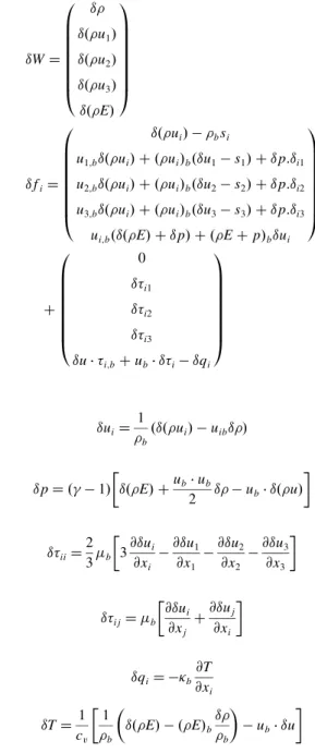
fluid Eqs. (1) by retaining only the first-order terms in the perturbation variables ("W). The subscript b stands in this part for the base variables, and the prefix " for the perturbation ones. Assuming the base state is a steady solution of Eqs. (1), the following equation is obtained: Vb @_!"W" @t # Wb @_!"V" @t $ %"R $ % @_!"Fi" @x_i (4) Because the flow perturbation variables and the wall motion ("M) are assumed to be harmonic at a pulsation !, the previously linearized Eqs. (4) can be written in the frequency domain as

8 > > > < > > > :

"W$ "W:ei!t_{; withi}2_{$ %1}

"M$ "M:ei!t_; "Fi$ "fi:ei!t; s_{$ i!:"M} i!Vb"W# i!Wb"V# @_!"fi" @xi $ 0 (5) where

"W_$ "! "_!!u1" "_!!u2" "_!!u3" "_!!E" 0 B B B B B B B @ 1 C C C C C C C A "fi$ "_!!ui" % !bsi

u1;b"!!ui" # !!ui"b!"u1% s1" # "p:"i1

u2;b"!!ui" # !!ui"b!"u2% s2" # "p:"i2

u_3;b"_{!!ui" # !!ui"b!"u}3% s3" # "p:"i3

ui;b!"!!E" # "p" # !!E # p"b"ui

0 B B B B B B B @ 1 C C C C C C C A # 0 "#_i1 "#i2 "#i3

"u_{& #}i;b# ub& "#i% "qi

0 B B B B B B B @ 1 C C C C C C C A and "ui$ 1 !b!"!!ui" % uib "!_" "p_{$ !& % 1"} # "_{!!E" #}ub& ub 2 "!% ub& "!!u" $ "#ii$ 2 3$b # 3@"ui @xi % @"u1 @x1 % @"u2 @x2 % @"u3 @x3 $ "#ij$ $b #_@"u i @xj # @"uj @xi $ "qi$ %%b @T @xi "T_$1 cv #₁ !b ! "_{!!E" % !!E"}b "! !b " % ub& "u $

The latter linearized fluid equation (5) has been obtained con-sidering the laminar and turbulent viscosity coefficients frozen to their base state. For a given base state, it yields a complex linear system in the complex variable "W, which is solved using a pseudo-time-implicit method (backward-Euler LU-SSOR) associated with local time-stepping and multigrid algorithms. The choice is naturally made to use the steady solution as a base state. It is computed separately for the zero-deflection position of the flap, and it is an input for the resolution of the system in the frequency domain.

D. Harmonic Balance Method 1. Fourier-Based Time Discretization

For a periodic flow, the first step in the HB method is to perform a Fourier decomposition of the flow variables and residuals [5,7]. The series are then injected in the semidiscrete form of the RANS equations Eqs. (1) to obtain a set of coupled equations in the fre-quency domain. A subset of these equations is solved up to mode N, the number of harmonics retained in the Fourier series. A discrete inverse Fourier transform is then used to cast back the system in the time domain. A set of mathematically steady equations coupled by a source term is finally obtained:

R_!Wn; sn" # Dt'!VW"n( $ 0; 0) n < 2N # 1 (6)

where the subscript n denotes a snapshot of a quantity at the instant t_{n$ nT=!2N # 1". These “steady” equations thus correspond to} 2N# 1 instants equally spaced within the period. The new time operator Dt connects all the instants and can be expressed

analytically as

D_{t''( $} X

N m$%N

d_m'_n#m (7)

where ' is a flow variable [' $ !VW" in Eq. (6)], with dm$ %( T!%1" m#1_csc!(m 2N#1"; m ≠ 0; 0 m_{$ 0}

The source term Dt'!VW"n( can be viewed as a high-order spectral

formulation of the initial time derivative in Eqs. (1). This spectral operator is applied to all the flow variables, including the turbulent ones.

Following the dual time-stepping approach, a pseudotime deriv-ative t*

nis added to Eq. (6) to time march the equations to the

“steady-state” solution for each instant.

For stability reasons, the computation of the local pseudotime step is modified [15] to take into account the HB source term. Here, the Block–Jacobi symmetric-overrelaxation implicit treatment of the HB source term proposed by Sicot et al. [9] is used.

Interestingly, the HB method could be viewed as the super-imposition of a high-order complex perturbation over a time-averaged solution (the zero-order term of the Fourier series), whereas in the LUR method, the base state is the steady solution, and the perturbation is of the first order; hence, there is some similarity between a LUR and a one-harmonic HB solutions.

2. Grid Deformation Velocity

An issue specific to the ALE approach is the computation of the mesh velocity snfor each instant. Although the use of the harmonic

approach within the ALE framework has already been presented in the literature [16], no mention is made of the way the mesh velocity is computed. Although sE

n can still be obtained using analytical

equations for the rigid-body movement considered, the mesh-deformation velocity needs special treatment.

Obviously, the accuracy of Eq. (3) depends on the ratio of the time step !t to the period of the problem. In a typical URANS calculation, at least 40 instants discretize the period, which yields an accurate evaluation of sD_{. In an HB calculation, the number of instants in the}

period (typically 3–11) cannot provide a good estimate of sD_using

this standard finite difference scheme, as illustrated later (see Fig. 1). For a transfinite interpolation approach with fixed outer boundaries, there is no analytical derivation of sD_{; therefore, an alternative is}

needed.

An efficient approach to evaluate sD_{is to apply the HB spectral}

operator to the coordinates of the mesh at the 2N # 1 instants: sD

n $ Dt'Mn( $

XN m$%N

dmMn#m (8)

The accuracy of this evaluation depends on the order N of the method, as does the accuracy of the whole HB approach. The kind of problem that can occur with the finite difference approach can be illustrated considering a simple pitching airfoil. The mesh velocity on the skin of the airfoil is geometrically linked to the instantaneous rotation speed:

)_{!t" $ sin!! & t"; and" !t" $}d)

dt$ ! & cos!! & t" Figure 1 compares the exact solution for the rotation speed with a 40-point finite difference solution, a three-point finite difference solution, and the N $ 1 HB operator solution. The three-point finite difference solution is not only far from the solution in terms of amplitude, but it has the wrong sign for the second instant of the period. At that instant in the period, the airfoil leading edge would

appear to be going up, whereas it is actually going down. In contrast, the HB (N $ 1) solution is very accurate.

E. Numerical Aspects

All the simulations are performed with the elsA software, a multi-application CFD flow solver that solves the three-dimensional Navier–Stokes equations using a finite volume cell-centered formul-ation on multiblock structured meshes [11]. Here, the spatial convec-tive fluxes are discretized by the second-order centered scheme with Jameson-type artificial dissipation [17]. Diffusive terms are com-puted with a second-order scheme. In the present study, two different models are used to compute the turbulent viscosity: the one-equation Spalart–Allmaras model [18], and the shear stress transport (SST) k–! model of Menter [19] with a Zheng limiter [20].

III. Results and Discussion

A. Test Cases and Setup

1. NACA 64A006 with Oscillating Flap

The test case considered here is a two-dimensional case proposed by AGARD, presented in [21]. It consists of a NACA 64A006 airfoil with a flap mounted at 75% of the chord. Several flow configurations are available in the AGARD data set for this geometry, depending on the incoming flow Mach number M1 and angle of attack )1, the

oscillation frequency f, and the maximum deflection angle "0. The

two cases retained for the present study are denoted as CT1 and CT6.

Another case has been considered, for which experimental data are not available. To provide a test case in the transonic regime with separation, the angle of attack of the CT6 case has been increased so that a detached flow is observed on the upper side of the flap. This case will be referred to as CT6-DF (for detached flow). All the test cases are summarized in Table 1.

2. Numerical Setup

The two-dimensional domain extends 30 chords upstream, downstream, below, and above the airfoil. The computational mesh is made of a C-type block around the airfoil and an H-type block for the blunt trailing edge. The C block has 354 nodes on the airfoil and 70 points in the normal direction. Close to the wall, the mesh refinement is such that about 25 points are located in the boundary layer, with a first cell height at y#+ 1. Downstream of the airfoil, 9 points are put across the blunt trailing edge, and 41 points discretize the wake in the streamwise direction. The total number of points is therefore about 30,000.

The boundary conditions are a nonreflecting far-field condition on the boundary of the domain and a no-slip adiabatic wall condition on the airfoil. The steady, URANS, and HB simulations are initialized by a uniform flow. Because the Spalart–Allmaras model has proven its efficiency in computing external attached flows, it was retained to run the simulations for the CT1 and CT6 cases. In the detached case, a very slow convergence of the turbulent field was observed, which improved using the SST k–! model of Menter.

B. Numerical Studies

The choice of the numerical parameters is of paramount importance when the performances of the methods are compared in terms of CPU time. For all the computations, iterative convergence for the LUR and HB calculations was monitored, as well as time accuracy for the URANS solution. The choice was made to monitor convergence on the basis of the unsteady pressure distribution. That is to say, a computation was considered converged when the first harmonic of the pressure distribution did not significantly change any further with the iterative process. It should be emphasized here that integrated forces can be converged faster than pressure distributions. The numerical parameters used for the different test cases are summarized in Table 2.

For the subsonic case (CT1), a smooth convergence was obtained for all the methods, as can be observed in Fig. 2. For the HB case, the fastest convergence was obtained with a linear increase of the Courant–Friedrichs–Lewy (CFL) number from 50 to 100 during the first 100 iterations.

For the transonic case (CT6), the number of time steps was slightly increased for the URANS case. For the LUR case, a low number of iterations still provided a good solution. For the HB case, the strategy of a linear increase of the CFL number was maintained, but the lower value of the CFL was reduced and the number of iterations was increased. The iterative convergence curves of the residuals for the LUR and HB methods are shown in Fig. 2.

-10 -5 0 5 10 0 0.2 0.4 0.6 0.8 1 Omega t/T exact solution 40-point finite difference 3-point finite difference HB operator N=1

Fig. 1 Comparison of the finite difference and HB operators to compute the derivative of a sinus.

Table 2 Numerical parameters for all the test cases

CT1 CT6 CT6-DF

URANS

Time step T=48 T=64 T=64

Number of simulated periods 3 3 3

Max. number of dual iterations 25 50 80

CFL number 50 50 50

HB N_{$ 1–3} N_{$ 4} N_{$ 5}

Number of iterations 250 300 800 1200 3000

Min. CFL number 50 5 1 1 1

Max. CFL number 100 100 50 10 5

Linear evolution range 50 50 100 200 500

LUR

Number of iterations 200 200 ——

CFL number 50 50 ——

Table 1 Description of the NACA 64A006 test cases

)₁, deg M₁ f, Hz "0, deg

CT1 0.0 0.794 30.0 1.09

CT6 0.0 0.853 30.0 1.10

In the transonic regime with detached flow (CT6-DF), converg-ence was somehow harder to obtain. For the URANS, the number of dual iterations had to be increased. In this case, it was not possible to obtain a converged solution with the LUR method. The matrix of the linear system Eq. (5), depending on the Jacobian matrices of the steady fluxes !@fi=@W", has eigenvalues for which the real part is

negative. Because this matrix remains constant during the resolution process, every time-marching algorithm will diverge exponentially in time. However, a solution could be computed using a generalized minimal residual method (GMRES) type of algorithm, or a direct resolution of the linear system, but at a possibly higher cost. Such methods are not yet implemented in the elsA code. For the HB method, the maximum CFL number was reduced to 10 for N $ 4 harmonics and to 5 for N $ 5 harmonics. It was therefore necessary to increase the number of iterations above three harmonics. Convergence difficulties when increasing the number of harmonics have already been reported in the literature [15], sometimes leading to divergence [5].

C. Physical Analysis

In this section, the physical accuracy of the results is analyzed. The comparison is focused on the pressure coefficient Cpdistribution

along the airfoil obtained by the three methods. To analyze the unsteady evolution of the pressure coefficient, the first harmonic Cp1

is computed. For the HB and URANS results, the mean value Cp0is

obtained from an arithmetic time average. For the LUR results, the steady solution is used for the comparisons.

It should be stressed here that the purpose of the paper is to assess the capability of the LUR and HB methods to reproduce the URANS results. Of course, comparisons with the experimental results are of interest, but are not the main focus of the study.

1. CT1 Case

In this case, the flow remains subsonic all around the airfoil, as shown by the mean value of the Cpin Fig. 3. The LUR and HB results

are perfectly superimposed on the URANS results. The computa-tional results are in good agreement with the experimental data.

The first harmonic of the Cpis shown in Fig. 4. For the real and

imaginary parts of the LUR and one-harmonic HB solutions, some slight differences can be observed. Altogether, these differences are negligible. For N $ 2, the HB solution is superimposed to the URANS results. Overall, the computational results are only in fair agreement with the experimental data. In [21], the authors mention a lack of rigidity of the flap, which could explain some of the discrepancies.

2. CT6 Case

In this case, the flow is transonic, with a shock alternatively forming on both sides of the airfoil, at about midchord. In Fig. 5, the steady solution associated with the LUR method is significantly different from the time-averaged solution, as expected for such a case with large shock motion (as shown later in this section; see Fig. 7). For the HB results, there is a noticeable influence of the number of harmonics: for N $ 1, there are some discrepancies with the URANS near the shocks; for N $ 2 these differences are negligible.

Considering the first harmonic of the Cppresented in Fig. 6, the

solutions differ around the shocks, but are identical in the rest of the flow. For the LUR, the amplitude of the peaks is overestimated, whereas the width is underpredicted. This point is discussed further later on. The behavior of the linearized method could be explained by the structure of the unsteady flow, as shown in Fig. 7: the URANS simulation shows that the shock moves along the chord, whereas the LUR method is only able to model a shock staying at its steady location. Another point is that the shock disappears and reappears within the period. This phenomenon is an unsteady nonlinearity, which cannot be properly modeled by the LUR method. For the HB solution, N $ 2 yields fair accuracy, and the solution is superimposed to the URANS reference for N , 3.

Despite minor discrepancies, Fig. 6 gives an empirical indication that the HB solution is better than the LUR solution in the vicinity of

10-7 10-6 10-5 10-4 10-3 10-2 10-1 100 0 50 100 150 200 250 Density residual Number of iterations LUR HB N=1 HB N=3 10-7 10-6 10-5 10-4 10-3 10-2 10-1 100 0 50 100 150 200 250 300 Density residual Number of iterations LUR HB N=1 HB N=3 10-7 10-6 10-5 10-4 10-3 10-2 10-1 100 0 500 1000 1500 2000 2500 3000 Density residual Number of iterations HB N=1 HB N=3 HB N=4 HB N=5 a) CT1 b) CT6 c) CT6-DF

Fig. 2 Convergence of the computations: mean residual of the density, normalized by the value at the first iteration.

-0.4 -0.3 -0.2 -0.1 0 0.1 0.2 0 0.2 0.4 0.6 0.8 1 Cp0 x/c EXP URANS HB N=1 HB N=2 LUR -0.4 -0.3 -0.2 -0.1 0 0.1 0.2 0 0.2 0.4 0.6 0.8 1 Cp0 x/c EXP URANS HB N=1 HB N=2 LUR

a) Upper side b) Lower side

shocks. Our theoretical explanations for this behavior are the following:

1) The main difference between the linearized and the one-harmonic methods is the step at which the one-harmonic truncation is done. In the LUR case, the equations are linearized before the numerical resolution. In the HB case, Eq. (6) retains all the nonlinear-ities of the spatial operators of the Navier–Stokes equations, and the truncation is done at the level of the resolution, via the number of harmonics retained. Indeed, in the HB technique, the residual R is computed by the same routines as in the nonlinear URANS approach. 2) A second difference is that the one-harmonic HB solution (and, of course, HB solutions of higher order) takes into account the true flap position at several different instants in the period, via the mesh deformation, thus allowing one to model, to some extent, shock motions.

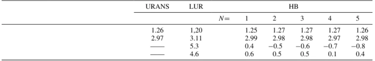
To further contrast the quality of the LUR and HB predictions, the unsteady aerodynamic forces are analyzed. One way to do this is to compute the generalized aerodynamic force (GAF). Harmonic analysis is performed on the unsteady GAF signal (nondimension-alized by the upstream dynamic pressure and the chord), and the modulus and phase of the first harmonic are presented in Table 3. As noticed before, the LUR overestimates the amplitude of the peaks and underpredicts their width: these errors cancel each other out after integration, and the unsteady force is predicted quite well, with about a 5% error. The HB results are within 1% of the URANS ones, whatever the number of harmonics.

Regarding the comparison of the numerical and experimental results, the first harmonic of Cpis fairly well predicted except around

the shock, where the peak is predicted downstream of the experi-mental location, with a significant overestimation of its magnitude.

-10 -5 0 5 10 0 0.2 0.4 0.6 0.8 1 Re[C p1 ] x/c EXP URANS HB N=1 HB N=2 LUR -3 -1.5 0 0.05 -10 -5 0 5 10 0 0.2 0.4 0.6 0.8 1 Im[C p1 ] x/c EXP URANS HB N=1 HB N=2 LUR -0.5 0 0.5 0.7 0.8 0.9 1

a) Real part b) Imaginary part

Fig. 4 CT1 case: first harmonic of the pressure coefficient, with a close-up view of the areas of interest.

-0.4 -0.2 0 0.2 0.4 0 0.2 0.4 0.6 0.8 1 Cp0 x/c EXP URANS HB N=1 HB N=2 LUR -0.4 -0.2 0 0.2 0.4 0 0.2 0.4 0.6 0.8 1 Cp0 x/c EXP URANS HB N=1 HB N=2 LUR

a) Upper side b) Lower side

Fig. 5 CT6 case: mean (URANS and HB) and steady (LUR) distributions of the pressure coefficient.

-20 -10 0 10 20 30 0 0.2 0.4 0.6 0.8 1 Re[C p1 ] x/c EXP URANS HB N=1 HB N=2 HB N=3 LUR -8 -6 -4 -2 0.4 0.5 0.6 -20 -10 0 10 20 0 0.2 0.4 0.6 0.8 1 Im[C p1 ] x/c EXP URANS HB N=1 HB N=2 HB N=3 LUR -6 -4 -2 0.4 0.5 0.6

a) Real part Imaginary part

Besides the remarks made in the preceding section, it can be added that the amplitude of the peaks is hard to measure accurately, because it requires a clustering of pressure taps in the areas where they occur. However, it is likely that some flow features could not be resolved by either the numerical strategies adopted or the mesh resolution used.

3. CT6-DF Case

This case is derived from the CT6 case: the flow is transonic and the angle of attack is increased to 4 deg, so that the flow is detached on the upper side of the flap. As mentioned earlier, in this case the LUR computation did not converge.

Figure 8 presents the flow computed by the URANS and the HB (N $ 1) methods. The two visualizations are snapshots at t $ T=3 (flap up, going down), with contours of the Mach number and some streamlines. This figure illustrates the size of the separation zone. It also shows the good agreement between the two methods with regard to the qualitative prediction of the flowfield.

The distribution of the mean value of the Cpis presented in Fig. 9

for the HB and URANS solutions. On both sides of the airfoil, all the HB solutions are superimposed to the URANS ones.

In Fig. 10, the real and imaginary part of the Cpare plotted for the

URANS and HB methods. An interesting point is that the HB solution does not change when the number of harmonics is increased over N $ 2. To account for this, the frequency content of the wall pressure at x=c $ 0:5 is examined (the point is located in the region where the shock moves). For the URANS, Fourier analysis is performed on the unsteady signal over five periods (after the initial

convergence stage). The results for the CT6 and CT6-DF cases are given in Fig. 11. Close agreement between the URANS and the HB results is found. It appears that the frequency content of the CT6-DF case is indeed much poorer than that of the CT6 case, hence the faster convergence of the HB in this case with regard to the number of harmonics. Our physical explanation is that the detached-flow area limits the amplitude of the unsteady motion of the shock.

D. Performance Analysis

As a preliminary, we note here that the initial motivation for the development of harmonic and linearized approaches is a reduction in the CPU time. However, little information on this issue is available. Hall et al. [5] compare their approach to steady computations, which is not suited to our case, because the goal is to substitute the HB computation with the URANS ones. Gopinath et al. mention a significant CPU reduction for turbomachinery applications (two orders of magnitude, but partly due to a domain reduction thanks to specific boundary conditions) [8], but they do not provide the equivalent information for external aerodynamics flows [7]. With a slightly different approach for the implicit treatment of the source term, Woodgate and Badcock [10] show a significant gain (about a factor of 10) as compared to URANS for external flows.

The restitution time is used to assess the performances of the methods. The gain is defined as the ratio between the URANS restitution time and the LUR/HB restitution time. For the LUR, the inclusion of the calculation time of the steady solution in the total time is a point of concern. In the present case, because a single

Fig. 7 CT6 case: snapshots of the flow computed by the URANS method.

Table 3 CT6 case: Comparison of the nondimensionalized generalized aerodynamic forces; analysis of the first harmonic

URANS LUR HB

N$ 1 2 3 4 5

GAF _{Modulus (-10}7_{) 1.26 1,20 1.25 1.27 1.27 1.27 1.26}

Phase, rad 2.97 3.11 2.99 2.98 2.98 2.97 2.98

Rel. error Modulus, % —— 5.3 0.4 %0:5 %0:6 %0:7 %0:8

operating point is examined and because the URANS and HB computations are initialized by a uniform field, the choice was made to include the calculation time of the steady solution in the total time. Figure 12 presents the gains obtained for all the test cases, plotted as a function of the number of harmonics used for the HB computations. To allow consistent comparisons of the methods, the gain of the LUR solution is plotted as a line on the same graph, although it does not depend on N.

For the subsonic test case CT1, the LUR is over seven times faster than the URANS, whereas the HB computations are up to four times faster than the URANS.

For the transonic test case CT6, the LUR is about eight times faster than the URANS. The fact that the LUR calculation time is not much reduced as compared to the CT1 case, in spite of an increased time for the URANS, is due to a longer steady computation. The N $ 1 HB is about six times faster than the URANS.

Fig. 8 CT6-DF case: color contours of the Mach number with streamlines.

-1 -0.8 -0.6 -0.4 -0.2 0 0.2 0.4 0.6 0.8 1 Cp0 x/c URANS HB N=1 HB N=2 -0.4 -0.2 0 0.2 0.4 0.6 0.8 1 0 0.2 0.4 0.6 0.8 1 Cp0 x/c URANS HB N=1 HB N=2

a) Upper side b) Lower side

Fig. 9 CT6-DF case: mean value of the pressure coefficient.

-3 -2 -1 0 0 0.2 0.4 0.6 0.8 1 Re[C p1 ] x/c URANS HB N=1 HB N=2 HB N=3 -6 -4 -2 0 2 4 6 0 0.2 0.4 0.6 0.8 1 Im[C p1 ] x/c URANS HB N=1 HB N=2 HB N=3

a) Real part b) Imaginary part

For the transonic test case with detached flow CT6-DF, the conclusion is that the HB is the only alternative to the URANS. For N_{, 2, the HB solution is no longer dependent on the number of} harmonics and is about three times faster than the URANS.

It should be emphasized here that the objectivity of the gain evalu-ation highly depends on the numerical parameters chosen for all the methods. For the subsonic case CT1, the gain is moderate because the URANS converges with a low time resolution and few dual itera-tions. For the transonic case CT6, the HB method is quite efficient because the robustness of the implicit approach [9] allows for large CFL numbers. For a number of harmonics below three, the HB method remains robust in the transonic test case with detached flow CT6-DF. Generally speaking, it is expected that the gain with the HB approach increases with the length of the URANS transitory phase. Regarding the memory requirements of the methods, the LUR requires only about 1.6 times the memory of the URANS. For the HB

technique, the memory cost for the one-harmonic computation is significant, about a factor of 3 compared to that of the URANS, and it scales linearly as the number of instants (i.e., a N $ 3 computation requires seven times the URANS memory).

IV. Conclusions

One of the reference approaches to predict unsteady aerodynamic loads is to perform URANS forced-motion simulations. The present study examines two alternatives to that technique, namely, the linearized method and the harmonic balance method. The assessment of these two methods against URANS predictions is carried out for a NACA 64A006 airfoil with a flap mounted at 75% of the chord for three flow regimes. Of particular interest is the fact that the same test case is evaluated over a range of significantly different flow condi-tions with varying levels of nonlinearities. Particular emphasis is put

10-5 10-4 10-3 10-2 10-1 100 Mean f 2f 3f 4f 5f 6f 7f Magnitude Frequency URANS HB N=1 HB N=2 HB N=3 HB N=4 HB N=5 10-5 10-4 10-3 10-2 10-1 100 Mean f 2f 3f 4f 5f 6f 7f Magnitude Frequency URANS HB N=1 HB N=2 HB N=3 HB N=4 HB N=5 a) CT6 b) CT6-DF

Fig. 11 Fourier analysis of the wall unsteady pressure at x=c ! 0:5. The URANS signal is analyzed over five periods.

0 2 4 6 8 1 2 3

Time Gain vs URANS

Number of Harmonics HB LUR 0 2 4 6 8 1 2 3 4 5

Time Gain vs URANS

Number of Harmonics HB LUR 0 2 4 6 8 1 2 3 4 5

Time Gain vs URANS

Number of Harmonics HB

a) CT1 subsonic case b) CT6 transonic

c) CT6-DF transonic detached flow

on the objective evaluation of the performances of the LUR and HB methods in terms of CPU time gain as compared to the URANS. All the simulations are performed within the ALE framework. For the HB technique, a specific approach for the computation of the mesh velocity is proposed, based on the same spectral operator as for the HB source term.

For the subsonic case CT1, it appears that the LUR method is the most appropriate one, because it is as accurate as the URANS method, with a computational time reduced by a factor of 7 as com-pared to the URANS and by almost a factor of 2 as comcom-pared to the HB (N $ 1). For the transonic case CT6, the choice depends on the level of accuracy required by the intended application: the LUR solution is obtained about eight times faster, but with poor accuracy around shocks, whereas the HB (N $ 1) solution is slower but more accurate. However, the discrepancies for the local pressure distrib-ution cancel each other out after integration, yielding a fair prediction of the unsteady force. For N $ 2, the HB is as accurate as the URANS, with a speedup of four. For the transonic case with separation over the flap CT6-DF, the LUR does not converge, and the HB (N $ 2) is quite accurate, with a speedup of about three. For the LUR method, a possible improvement to get a solution for the detached case would be the use of a GMRES-like algorithm, or a direct resolution of the linear system, which are not implemented in the solver used for the present study. These are topics currently under investigation.

One important result is that the one-harmonic HB solution is able to capture unsteady nonlinearities that the LUR solution fails to predict. We contend that the theoretical basis for this behavior is the following:

1) The nonlinearities of the spatial operators of the Navier–Stokes equations are preserved in the HB formulation, whereas the LUR solves a linearized set of equations.

2) The one-harmonic HB takes into account three different meshes in the period, whereas the LUR computes the solution on the initial mesh only.

3) The “pseudo base state” on which the one-harmonic perturbation is superimposed is the time-averaged state for the HB, whereas it is the steady-state solution for the LUR, which may differ when significant unsteady effects occur.

As far as practical aspects are involved, it should be emphasized that the LUR and HB methods have a lower setup cost than the URANS, because it is easier to monitor iterative convergence than time accuracy.

References

[1] Hall, K. C., “A Linearized Euler Analysis of Unsteady Flows in Turbomachinery,” Massachusetts Inst. of Technology Gas Turbine Lab. Rept. 190, 1987.

[2] Clark, W. S., and Hall, K. C., “A Time-Linearized Navier–Stokes Analysis of Stall Flutter,” Journal of Turbomachinery, Vol. 122, No. 3, July 2000, pp. 467–476.

doi:10.1115/1.1303073

[3] Mortchéléwicz, G. D., “Aircraft Aeroelasticity Computed with Linearized RANS Equations,” Technion—Israel Institute of Technol-ogy Paper 34, Feb. 2003.

[4] Liauzun, C., Canonne, E., and Mortchéléwicz, G. D., “Flutter Numer-ical Computations Using the Linearized Navier–Stokes Equations,” Advanced Methods in Aeroelasticity, NATO Research and Technology

Organisation, Rept. RTO/AVT-154, May 2008.

[5] Hall, K. C., Thomas, J. P., and Clark, W. S., “Computation of Unsteady Nonlinear Flows in Cascades Using a Harmonic Balance Technique,” AIAA Journal, Vol. 40, No. 5, May 2002, pp. 879–886.

doi:10.2514/2.1754

[6] He, L., and Ning, W., “Efficient Approach for Analysis of Unsteady Viscous Flows in Turbomachines,” AIAA Journal, Vol. 36, No. 11, Nov. 1998, pp. 2005–2012.

doi:10.2514/2.328

[7] Gopinath, A., and Jameson, A., “Time Spectral Method for Periodic Unsteady Computations over Two- and Three-Dimensional Bodies,” AIAA Paper 2005-1220, Jan. 2005.

[8] Gopinath, A., Van der Weide, E., Alonso, J., Jameson, A., Ekici, K., and Hall, K., “Three-Dimensional Unsteady Multi-Stage Turbomachinery Simulations Using the Harmonic Balance Technique,” AIAA Paper 2007-0892, Jan. 2007.

[9] Sicot, F., Puigt, G., and Montagnac, M., “Block–Jacobi Implicit Algorithms for the Time Spectral Method,” AIAA Journal, Vol. 46, No. 12, Dec. 2008, pp. 3080–3089.

doi:10.2514/1.36792

[10] Woodgate, M., and Badcock, K. J., “Implicit Harmonic Balance Solver for Transonic Flow with Forced Motions,” AIAA Journal, Vol. 47, No. 4, April 2009, pp. 893–901.

doi:10.2514/1.36311

[11] Cambier, L., and Veuillot, J., “Status of the elsA Software for Flow Simulation and Multi-Disciplinary Applications,” AIAA Paper 2008-0664, Jan. 2008.

[12] Jameson, A., “Time Dependent Calculations Using Multigrid, with Applications to Unsteady Flows Past Airfoils and Wings,” AIAA Paper 1991-1596, 1991.

[13] Yoon, S., and Jameson, A., “An LU-SSOR Scheme for the Euler and Navier–Stokes Equations,” AIAA Paper 87-0600, Jan. 1987. [14] Delbove, J., “Unsteady Simulations for Flutter Prediction,”

Computa-tional Fluid Dynamics 2004, Springer, Berlin/Heidelberg, 2006, pp. 205–210.

doi:10.1007/3-540-31801-1_26

[15] Van der Weide, E., Gopinath, A., and Jameson, A., “Turbomachinery Applications with the Time Spectral Method,” AIAA Paper 2005-4905, June 2005.

[16] Thomas, J. P., Dowell, E. H., and Hall, K. C., “Nonlinear Inviscid Aerodynamic Effects on Transonic Divergence, Flutter, and Limit-Cycle Oscillations,” AIAA Journal, Vol. 40, No. 4, April 2002, pp. 638– 646.

doi:10.2514/2.1720

[17] Jameson, A., Schmidt, W., and Turkel, E., “Numerical Solutions of the Euler Equations by Finite Volume Methods Using Runge–Kutta Time-Stepping Schemes,” AIAA Paper 81-1259, June 1981.

[18] Spalart, P. R., and Allmaras, S. R., “A One-Equation Turbulence Transport Model for Aerodynamic Flows,” AIAA Paper 92-0439, Jan. 1992.

[19] Menter, F. R., “Zonal Two Equation (k–!) Turbulence Models for Aerodynamic Flows,” AIAA Paper 93-2906, July 1993.

[20] Zheng, X., Liao, C., Liu, C., Sung, C. H., and Huang, T. T., “Multigrid Computation of Incompressible Flows Using Two-Equation Turbu-lence Models: Part I—Numerical Method,” Journal of Fluids Engineering, Vol. 119, 1997, p. 893–899.

doi:10.1115/1.2819513

[21] “Compendium of Unsteady Aerodynamic Measurements,” AGARD R-702, 1982.

N. Wereley Associate Editor