The performance of banks during the financial crisis

(1)

Pierre-Emmanuel CAUSSE

Reference number 16,624 HEC 2011

The performance of banks during the financial crisis

A study of European banks market and operational performance drivers from the bust of

the subprime crisis to the end of 2009.

Referent Professor:

(2)

(3)

Abstract

This master thesis aims to investigate the drivers of European banks market and operational performance during the financial crisis. We study market performance over three periods of time: the pre-Lehman bankruptcy phase (from August 2007 to September 2008), the core-downturn phase (from September 2008 to March 2009) and the post core-crisis recovery (from March to December 2009). We find that during the first period, banks were mostly sold indiscriminately even though there are evidences for some focus on size and on the level of capitalization. In the second phase, best performers were banks with traditional and cautious business models implying a large weight of loans and liquid assets within the balance sheet. In a swing movement, investors turned back to more risky profiles in the third period. We also study the determinants of operational performance in 2007, 2008 and 2009. We find that 2007 most resilient institutions were those which combined conservative business models with high pre-crisis RoTE. These two factors remained determinant in 2008 and the proportion of liquid assets also appeared as a significant driver. Our 2007 and 2008 results might suggest the existence of a “best-in-class management” effect. In 2009, the key drivers of banks performance were previous year return on equity and level of capitalization. This might highlight the durable positive effect of the preservation of robust business foundations in a historically tough environment. Before going through the details of this study, we provide our reader with a brief presentation of the main business, accounting and regulatory characteristics of banking institutions. Our work fills a gap in research as European banks had not been studied separately so far. Our approach based on the study of the determinants of both market and operational performance had to our knowledge, not been implemented before.

(4)

(5)

freeze three structured-credit-based funds because market conditions had made it impossible to compute their net asset value. This decision caused the almost-total stopping of the interbank lending market, forcing the European Central Bank (ECB) to immediately inject €95 billion to allow banks to refinance themselves. These events were the beginning of the toughest financial crisis since the Great Depression, driving the S&P500 from 1,497.49 points

on the 8th of August 2007 to 676.53 points on the 9th of March 2009. Over the same period,

the Stoxx Banks TMI Index, which brings together the largest listed European banks, fell from 423.94 to 81.69 points.

In this research, we focus on the performance of the 86 banks composing the Stoxx Banks TMI index. Our work is also exclusively dedicated to the largest European banks, which have to our knowledge, not been studied separately so far. We consider two types of performance: a market performance measured by stock returns and an operational performance measured by pre-tax profit on average tangible assets. This metric captures both net revenue trends (i.e. general business evolution) and the evolution of the loan losses provision line (i.e. quality and risk of assets held in the balance sheet) which is the most cyclical one of a bank income statement. Moreover, it allows to us estimate the amount of assets necessary to generate pre-tax profit and can therefore be seen as a proxy for the return on capital employed often used for industrial firms. We then explore the possible relationships between these performance indicators and five classes of potential determinants: business model, balance-sheet structure, risk-management policy, liquidity characteristics and compliance with regulatory capital requirements.

Since March 2009, stocks markets and real economies have partially recovered. However, knowing whether the financial crisis is over or not is unclear as the U.S. real-estate market remains depressed, whereas European banks face new threats stemming from sovereign debts. Moreover, banks globally will have to reimburse or to refinance €2,418.5 billion within the next two years. As a result, we lead our investigations on a period going

from the 8th of August 2007 to the 31st of December 2009. We run our analysis on market

performance over three different periods of time: the first one goes from the 8th of August to

the day before the bankruptcy of Lehman Brothers on the 15th of September. The second

period goes from the collapse of Lehman Brothers to the markets low point in early March

2009. We finally study the recovery phase from the 9th of March 2009 to the end of 2009.

Investigations on operational performance are led using pre-tax profit on average tangible assets of fiscal years 2007, 2008 and 2009. We do not go until December 2010 because the fiscal year 2010 financial information of some of the banks from our sample is not currently available in Bankscope.

We identified a swing movement on market performance determinants. In the first period, the sector was mostly sold indiscriminately even though size and capitalization level appeared as significant drivers of performance. During the second phase, best performers had the most traditional business models with a large proportion of loans and liquid assets in their balance sheets. In the last period, investors privileged again risky and leveraged profiles. Operational performance was determined by business model conservativeness in both 2007 and 2008 but also by the level of RoTE. We interpret this finding as a possible sign of the existence of a “best-in-class” management effect. In 2008, liquidity of assets became an additional driver of operational performance. The following year, the key drivers of banks performance were 2008 return on equity and level of capitalization, suggesting a durable positive effect of the preservation of a strong operational efficiency despite the crisis.

(8)

Besides understanding what have been the drivers of banks performance during the crisis, the aim of this paper is also to provide our reader with a brief and as precise as possible presentation of how banks work. During our researches, we have indeed been looking unsuccessfully for a complete and easy to understand introduction to banks. Our ambition is also to design such a tool in the first part of this work. These few pages make the design and results of our performance analysis easier to understand.

In the first part of this paper, we expose the fundamental characteristics of European banks (I). We then present the details our analysis on potential banks operational and market performance (III). We finally expose our robustness checks, the synthesis and the limits of our findings

I. Fundamental characteristics of European banks: activities, accounting and regulatory environment, and business models

Banks ontologically differ from other companies by the nature, the complexity and the size of their activities which can lead to worldwide destabilization in case of failure. As an example, BNP Paribas’s total assets amounted to €2,057.6bn at end-2009 whereas French GDP was €1,850bn. This explains why banks have to follow specific accounting and regulatory rules. In this first part, we give the main lines of banks activities and accounting rules (1). We then explain how financial statements are adjusted for risk (2) and the main indicators to monitor when looking at banks financial statements (3). We finally examine the impact of pre-crisis changes in business models (4).

1. Banks activities and the way they are translated in the financial statements

This section exposes the basics of banks activities and accounting principles which differ significantly from the ones of other economic players primarily because banks use money as their raw material. We briefly recall the definition and functions of banks (1) before going through the main characteristics of their income statement (2) and of their balance sheet (3). We conclude this section by going through the main indicators to focus on when analyzing banks financial statements (4).

1.1. Banks: definition and functions within the economy

The definition of a bank varies from a country to another and there is surprisingly no European-wide regulatory definition of the word. However, a generally-admitted principle is that a bank is a company that is allowed to collect redeemable deposits from the general public and which conjointly runs lending activities and offers other diversified financial services. For instance, under French law, “banking operations include collecting funds from

the general public, credit operations, and providing and managing payment means”1

. Under British regulation, a bank is “a firm with a Part IV permission which includes accepting

deposits and which is a credit institution…”2.

Within these legal frameworks, banking institutions are very different from one to another but they all assume at least one of the following three fundamental roles in the economy. First of all, banks offer a safe place for money deposits which are guaranteed by banks themselves but also by European States which have elaborated insurance plans to protect depositors up to a certain point in case of an institution bankruptcy. By end-2011, European banks will have to

1

Code Monétaire et Financier, Article L311-1

2

(9)

guarantee their customers deposits up to €100,0003. The second role of banks is to make payments easier and more reliable by providing their customers with increasingly secured and dematerialized payments devices, and therefore to encourage trade development. Their last and most important function is to intermediate liquidity and credit risks by collecting short-term deposits on a large scale and turning them into (long-short-term) funding resources for retail and corporate borrowers.

1.2. Understanding a bank Profit & Loss (P&L) statement

Despite the high number and technicality of banking activities, it is possible to split banks revenue sources between two distinct categories:

- Interest-related revenue, i.e. interests earned on loans and credits. Most of the time, interests paid to customers and lenders are withdrawn from gross interest revenue and banks first report their net interest revenue.

- Non-interest revenue, which mostly include commissions on brokerage, trading and advisory, but also fees charged on customers for the use of their payment means. Earnings from proprietary trading are also accounted under this denomination.

Net interest revenue and non-interest revenue together form the net revenue, which is often the first line of a bank income statement and is equivalent to the gross margin of a traditional company.

This split is however imperfect as trading gains on interest-related products are recorded under the non-interest revenue category. More importantly, most European banks publish their financial statements following International Financial Reporting Standards

(IFRS), which begets that they have to comply with the well-known IAS 394 (to be replaced

by IFRS 9 by the end of 2011) on Financial Instruments. According to IAS 39, financial instruments have to be marked-to-market, including derivatives instruments that are not used to hedge a precisely-identified risk. Matching together an individual risk with an individual hedging derivative is often difficult as a single derivative may be used to cover several risks, such as different credits with comparable default risks and maturities. As a result, banks can be led to book virtual gains on their hedging strategies which may artificially inflate their net revenue. The split between pure operational revenue and IAS-39-revenue was not available in Bankscope for any of the institutions constituting our sample.

Lower in the income statement, come banks operating costs. They are mainly fixed and made of IT and personnel costs. Network expenses are also a significant part of institutions running a large retail business. Given this fixed cost structure, banks have an important operational leverage which makes their pre-provision margin (net revenue minus operating expenses) highly cyclical and very sensitive to changes in net revenue. However, the pre-provision profit is a poor indicator of a bank performance as it does not account for the level of risk the bank has been supported in order to generate its revenue and does not give any color on the quality of the loan portfolio and of trading books.

The only indicator of the underlying business risk that appears in a bank income statement is the loan losses provision line. It accounts for the amount of granted credits that are not expected to be reimbursed, or for which partial or total default has already been observed. This line is the most cyclical one of a bank income statement as it may, depending on the economic cycle and provision policy, be close to zero or reach up to 50% of net revenue in a depressed economic environment. By withdrawing the loan losses provision from the pre-provision profit, one obtains the operating income.

3

See the press release issued on the 24 May 2011 by the Committee of Economic Affairs of the European Parliament

4

(10)

Below the operating income profit, a bank P&L becomes similar to the one of traditional companies even though there is naturally no financial profit line. By withdrawing income taxes and the share of consolidated profit attributable to minority shareholders, one obtains the group net income.

1.3. Understanding a bank balance sheet

Starting from the liabilities side, the specificity of a bank balance sheet compared to traditional firms is the small weight of equity compared to the whole size of the balance sheet (6.23% average Equity to Total Assets ratio for the banks of our sample in December 2006, 5.44% in December 2009). This is explained by the fact that banks can access funding sources that are unavailable to other economic players, especially on the very short-term. As already said, under most European national laws, a bank is defined as a company that can collect money from the public at large. A consequence is that banks can, besides equity, rely on deposits collected from their customers to fund themselves. These deposits include all types of retail and corporate deposits but also the money that is entrust to banks’ asset management branches. Even though they can actually be long term resources, customer deposits are booked as short-term funding because they can virtually be withdrawn at a glance in case of a bank run.

To fund the gap between their short-term resources and their short-term funding needs, banks heavily rely on the interbank market, also known as the wholesale funding market. Available funding tools include interbank loans, money market instruments and repurchase agreements (repos). Money market instruments include certificates of deposits (CD) and commercial papers (CP). Certificates of deposit are contracts which acknowledge that a certain amount of money has been deposited for a certain time and will be reimbursed with interest at the end of the period whereas commercial papers are unsecured notes that allow well-rated borrowers to issue debt for less than 270 days. Interbank loans are often implemented over very short periods of time, from a few hours to a few days. Repurchase agreements allow a bank to sell some of its assets to another institution for a given short period of time. At the end of the repo contract, the borrowing bank repurchases its assets and pays an interest to its counterparty. Because of repos, banks balance sheets sometimes do not give a faithful view of their financial health as a bank running through difficulties can sell through a repo contract low-quality assets against cash just before the closing of the fiscal year. These assets are then repurchased just after the closing of the accounting period. Conceptually, repos are closed to another type of interbank money market instruments known as secured loans, where the lender receives collateral pledged by the borrower.

Banks also issue large amounts of term debt either as bonds, hybrid debt instruments (convertibles) or subordinated debt. These issuances had reached considerable levels in the years before the crisis of August 2007. From EUR365 billion in 2002, the amount of gross debt issued by European banks climbed to €1,100 billion in 2007. As a result, the volume of

debt to be reimbursed increased considerably until 2008 (up to €869 billion5

) and will continue to do so in the coming years (as banks will have to reimburse or to refinance

€2,418.56

billion within the next two years).

However, most of the risks borne by a bank institution come from the asset side of the balance sheet because all assets expect cash face credit, market or liquidity risk. As a result and given the already-mentioned limited size of the equity, major one-off trading losses associated with an increase in the default rate of borrowers can rapidly dry up all of a bank

5

This figure and the two previous ones have been estimated by Deutsche Bank

6

(11)

equity reserves (cf. Societe Generale emergency €5.5bn capital increase in February 2008 as a consequence of a record-breaking €4.9bn trading loss in January 2008) . A significant part of the balance sheet is made of net loans (i.e. gross loans minus reserve for impaired loans) granted to retail and corporate customers. The remaining part of the balance sheet includes trading books (proprietary or on behalf of clients) and hedging instruments. Tradable securities are accounted for at their market value as demanded by IAS 39. This leads to several pricing issues when, under certain market conditions, entire classes of assets become suddenly illiquid. Another consequence of the wide use of fair value is that the balance sheet is a very punctual view of a bank assets and liabilities which are by nature fast-moving and volatile.

1.4. Key performance indicators to monitor when looking at banks financial statements

A very commonly used indicator of banks profitability is return on tangible equity (RoTE). Goodwill is withdrawn of equity in the computation. Some banks may report RoTE beyond 40% but the average for banks in our sample is between 15% and 20%. This ratio is however imperfect as it can be artificially inflated by investing in risky activities or by excessively leveraging the balance sheet to benefit from the gearing effect. This metric is most significant when compared to the cost of equity as it can indicate the ability of an institution to create value for its shareholders.

From a more operational point of view, it is important to monitor the costs to income ratio and loans losses provision as a share of net revenue. The first metric is computed by dividing a bank IT, personnel and other expenses by its total income. The classical value of this ratio is between 55% and 70% for the banks of our sample. It is an important point to monitor in a normal economic environment as tight costs control is an effective way to increase pre-tax profit. The loans losses provision to net interest revenue ratio is the most cyclical one of a bank income statement. It may be very close to zero in a dynamic economic environment but may exceed 50% in a depressed environment. It is a precious indicator of the quality and risk of the underlying loan portfolio.

When examining the balance sheet, a first point to focus on is the growth in loans and to see how this growth has been financed. If loans have increased faster than deposits, the gap is likely to have been full by recourse to the wholesale market, which might have introduced more risk in the balance sheet. It is also interesting to monitor the growth in RWA and to compare it to the change in RoTE. As sharp rise in RoTE associated with a same movement of RWA is a sign that returns have been generated through increased risk taking. Another important metric is the Loan Losses Reserve to Gross Loans ratio. It first makes it possible to comprehend risks associated with the loan portfolio. Secondly, the loan losses reserves may be used as a safety cushion in case of an economic downturn as part of the amount can be reversed to smooth the negative effect of increasing gross loan losses provisions in the P&L. Traditionally, banks tend to increase their loans losses reserve at the end of the economic cycle.

The last important class of indicators to focus on is capital ratios. The level of equity to total assets allows us to assess the ability of a banking institution to absorb potential losses. It is also a proxy for the risk of its funding policy. Finally, a close monitoring of regulatory capital ratios is essential, especially of Tier 1 capital. If a bank does not meet the required criteria, it may have to launch a significant and dilutive capital increase to reinforce its capital structure. Changes in regulation regarding regulatory requirements deserve careful monitoring as they may significantly affect banks ability to invest in capital-costly risky activities and to generate high returns. We study the details of these requirements in the next section.

(12)

2. Risk-adjusted information and capital adequacy requirements

The first pillar of Basel II Accords7 (adopted in July 2004) which was in force when

the financial crisis burst had identified operational risk, market risk and credit risk as the three main dangers faced by banking institutions. Illiquidity of certain assets included in banks balance sheets had not been pointed out as a threat deserving dedicated monitoring and indicators at this time. As already explained banks assets are made of loans and trading books which all include credit and/or counterparty risks. Banks also bear large off-balance sheet commitments which do not appear in the financial statements despite a significant weight compared to the size of the balance sheet. In this part, we describe how banks account for the underlying risk of their in-and-off balance sheet assets (1), which capital requirements they

have to meet (2) and the new liquidity requirements imposed by Basel III8 regulatory

framework (3).

2.1. Computation of risk-weighted assets (RWA)

Basel Committee successive decisions have been intending to develop tools able to give a more faithful representation of risks borne by banks, both in-and-off balance sheets. The most important of these monitoring devices is risk-weighted assets (RWA). Under Basel II, there were two main ways to compute RWA:

- the Standardized Approach, which can be applied by any bank. Under this methodology, each claim is given a weight as a percentage of its face value. This weight depends on the nature and on the credit rating of the borrower and is predefined by the Bank of International Settlements (BIS). As an example, a 100-face-value bond issued by AAA-ranked sovereign issuer will account for 0 in the RWA computation. On the contrary, a 100-face-value claim on BB-ranked corporate issuers will account for 150 in the RWA calculation. The standardized approach also takes into account off-balance sheet items which are converted into credit exposure equivalents (CCE) through the use of credit conversion factors (CCF). As an example, a commitment with maturity below one year will be granted CCF 50% whereas a liability with maturity superior to one year will be given CCF 20%. Cancellation conditions also influence the level of CCF retained. If they are very favorable to the bank, they can justify a 0% CCF.

- the Internal-Ratings Based (IRB) Approach: this methodology is only available for institutions which meet a certain number of conditions and have been authorized by their regulator to use the IRB approach. Under this framework, components of credit risk are estimated by banks proprietary models. Each bank has to split all its credit exposures between five categories (corporate, sovereign, bank, retail and equity). The category determines the risk-weighted functions used to compute risk-weighted assets. Depending on the asset class, the calculation may become highly sophisticated. For each claim, the bank has to evaluate the probability of default (PD), the loss given default (LGD), the exposure at default (EAD) and the effective maturity (M). If necessary, the regulator may force an institution to adopt a pre-established value for one or several of these parameters.

The computation of risk-weighted assets has suffered no major change under Basel III reform.

7_{Basel Committee, 2004, “Basel II: International Convergence of Capital Measurement and Capital Standards: a Revised Framework”,}

Basel, Switzerland, April.

8_{Basel Committee, 2010, “Basel III: “A global regulatory framework for more resilient banks and banking systems”, Basel, Switzerland,}

(13)

2.2. Computation of minimum capital requirements

The point of RWA is to determine banks capital requirements supposed to mitigate bankruptcy risk. Basel II distinguished two types of potential regulatory capital:

- Core Capital (Tier 1), which is made of shareholder equity, legal reserve and retained earnings. Tier 1 capital must account for at least 50% of a bank capital base.

- Supplementary Capital (Tier 2): Tier 2 Capital can bring together, under certain conditions and depending on countries, undisclosed reserves, general provisions reserves, hybrid debt instruments (convertible bonds) and subordinated long-term debt. The total amount of Tier 2 capital cannot exceed 100% of Tier 1.

- Subordinated short-term debt covering market risk (Tier 3): subordinated short-term debt can be regarded as Tier 3 capital if it can be transformed into permanent capital immediately in case the bank needs it. Tier 3 capital cannot exceed 250% of a bank Tier 1 Capital, meaning that roughly 29% of bank underlying risk has to be burden by Tier 1 capital at all times.

The total capital ratio shall not fall below 8% of RWA, with at least 50% of regulatory capital made of Tier 1 resources.

Minimum capital requirements have faced several changes under Basel III. Even though total capital ratio has been left unchanged at 8% of RWA, efforts have been made in order to improve the quality of the underlying capital. Tier 1 capital has now to be at least equal to 6% of RWA at all times. A new subcategory of Tier 1 capital known as Common Equity Tier 1 Capital has been created. It is only made of banks common shares and retained earnings and must account for at least 4.5% of RWA.

Moreover the various ways to compute RWA has led banks to underestimate their risk exposure. Basel III also introduced a Leverage Ratio, computed by divided Tier 1 Capital by all in-and-off balance sheet commitments, generally taken at their accounting value. Off-balance sheet items will enter for 100% of their face value in the Leverage Ratio computation. The Leverage Ratio will be fully implemented in January 2018. However, all European banks will have to meet a 3% Tier 1 Leverage Ratio by January 2013.

2.3. Liquidity constraints introduced by Basel III Accords

Basel II Accords considered that high capital adequacy ratios were sufficient to allow banks to find the liquidity they need in every situation, including a financial crisis, as these ratios were supposed to be sufficient to reassure liquidity providers on the capacity of a given institution to survive a severe downturn. Neither a total freezing of the interbank lending market nor the complete illiquidity of whole classes of assets had been considered in 2004. To better monitor liquidity risk, Basel III agreements introduced two important indicators:

- the Liquidity Coverage Ratio (LCR): the LCR is design to measure a bank resilience to a thirty-day disturbance in its access to liquidity. This ratio is computed by dividing the stock of liquid assets (cash and eligible government, corporate and covered bonds) by 30-day cash outflows in a crisis situation. 30-day cash outflows include 7.5% of stable retail deposits, 15% of less stable deposits and 25% of corporate deposits. 100% of net additional funding obtained over the period is deducted from the amount of outflows. This ratio will be introduced in 2015 and its minimum level has not been fixed yet. However, it should not exceed 10% .The computation will be made assuming a disturbance in the access to liquidity by far less violent than during the last financial crisis.

- the Net Stable Funding Ratio (NSFR). The NFSR has been designed to curb over-reliance on short-term wholesale funding and to encourage a better adequacy between funding and liquidity characteristics of bank assets. The ratio is computed by divided Stable Funding

(14)

(namely Tier 1, long-term debt and weighted deposits) by Stable funding requirements (weighted loans and trading books). As for the LCR, the NFSR reference value has not been decided yet and will not be before 2018 even though it will for sure have to be not lower than 100%, meaning that stable funding shall be superior to loans and trading books.

As these ratios have not been implemented yet, we were not able to test them per se in our statistical study. However, we have used a proxy for an inverted NSFR, the Net Loans to Short-term Funding and Deposits ratio.

3. Banks operational and market behavior throughout the economic cycle

In this section, we describe the typical operational behavior of banks through the expansion, stabilization and depression phases of the economic cycle (1). We also explain on which levels they trade through the cycle and what metrics the market looks at depending on the economic environment (2).

3.1. Key drivers of banks operational behavior through the economic cycle

Two very important drivers of a bank operational performance in terms of profitability are GDP growth and the level of interest rates (See Spick, 2010). In a dynamic economic environment, the volume of wealth increases, which allow banks to collect more deposits. On the other hand, confidence in the future increases investments of households and companies, which increases the demand for loan and support investment banking activities. In a favorable economic context, the level of default among banks customers is also lower. As a result, GDP growth has a positive effect on net revenue but also, lower in the income statement, on the loan losses provision line. Given banks fixed-costs structure, an increase in the net revenue line combined with a decline in the loan losses provision has a powerful positive effect on banks margins and on RoTE.

Interest rates are also critical to banks performance. Contrary to the GDP, increasing interest rates negatively affect banks performance. Indeed, they determine the price at which banks grant loans but also the amount of interests they have to pay in order to secure wholesale short-term funding. Moreover, higher interest rates increase the default rate of unhedged floating-interest loans, with a straightforward negative effect on the loan losses provision line. Finally, interest rates influence the level of discount rates used to price assets at fair-value in the financial statements and have a negative effect on the cash price of financial assets, paving the way for lower non-interest related revenue. Low interest rates context is favorable to banks in the way that it drives GDP up rather than because they allow banks to benefit from the spread between short and long term maturities which tend to widen in this context. Indeed, no arbitrage constraints should assure that there is no difference between interests gained from holding a long-term bond and interests paid to secure short-term financing over the lifetime of the long short-term bond.

Because of their operational characteristics, banks are early-starters in the economic cycle and do amplify its trends. At the beginning of the expansion period of the cycle, banks enjoy strong profitability as demand for loans increases, financial markets recover and refinancing conditions are unusually clement. This encourages an increase in the size of banks balance sheets. Banks with the most strongly leveraged balance sheets tend to deliver higher profitability on the back of more powerful gearing effect. During the stabilization face, market growth slows down and rising interest rates make credit less attractive for borrowers. In this period, banks operational performance depends on more microeconomic issues including the degree of competition in the sector and the ability of operational teams in all business divisions to strictly control costs. Finally, the progressive rise in interest rates initiated by

(15)

central banks in order to curb inflation risks slows down balance sheet expansion and economic upturn. Harder situation for companies and households increase the default rate and reduce non-interest revenues, leading to the already explained scissor effect on the operating margin.

3.2. Banks market behavior and metrics

Along with operational behavior, banks market valuation faces several changes during the economic cycle. On the contrary to other companies, the concept of enterprise value does not exist for banks because it would be impossible to define banks net debt given their funding particularities. This explains why all bank-relevant ratios are based either on equity book value or on market capitalization. In a depressed environment, banks net profit may rapidly become negative or close to zero, making Price/Earnings (P/E) ratio irrelevant. Investors also focus on price to book value and more often price to tangible book ratios (P/TBV). During the crisis, it fell to 0.6x on average for the banks we studied whereas it reached 2.0x in 2007. A P/TBV below 1 indicates that investors virtually price in a bankruptcy as they think the fair value of the company is below its book value. In the middle of the cycle, banks tend to trade on average on 10.5x next-twelve-month P/E. On the eve of the crisis, the average next-twelve P/E was 12.1x and fell to 5.6x at the low point of the downturn. This metric can reach very high levels during the recovery phase as next-twelve-month expected earnings are still low whereas share prices rebound sharply. Investors also focus on very specific sector multiples that are beyond the scope of this paper.

Attention of investors is focused on the most leveraged banks during the beginning of the economic cycle as they are the most likely to benefit from low interest rates. During the stage level, investors regard banks as more traditional companies and therefore focus on the growth rate of earnings per share (EPS) to make their decision. When the downturn occurs, they tend to adopt a behavior opposed to what it has been during the recovery phase.

4. Pre-crisis changes in banks business models

In the years before the crisis, European banks business model has generally faced numerous and deep transformations, moving from an “Originate and Hold” to an “Originate, Repackage and Sell”. Traditionally, European banks used to keep loans and their inherent risks until maturity, the part of on-interest revenues being relatively modest, as pure large, US-style investment banks were virtually absent from the European landscape. Development of securitization techniques have allowed European banks to increasingly stream out of their balance sheets pools of credits that were then transferred to investors ready to bear default risk associated with these loans. Across Europe, the amount of securitization issuance grew from

€140bn in 2001 to €531bn in 20079

. This phenomenon has, along with other factors, led to a rise in the share of non-interests revenues within banks income statement. Other factors include the rapid development of additional investment banking activities which are by nature more profitable but also more volatile than classic commercial banking businesses (see Tumpel-Gugerell, 2009).

A consequence of the increased weight of non-interest activities is a transformation in banks balance sheet structure. Trading books share in the asset side has increased at the expenses of loans. This has little by little led banks to store assets which would prove impossible to price because they had become illiquid, implying large assets write-offs which have consumed huge proportion of banks equity. On the liability side of their balance sheets,

9

(16)

banks have also increasingly relied on non-deposit funding, namely wholesale market financing, in a context of abundant liquidity driven by low interest rates (see Pereiti 2010). As an example, the average Total Assets to Total Deposits ratio of European banks climbed from roughly 1.60% in 2001 to more than 2.00% in 2007. In a vicious circle, endless liquidity resources fuelled the growth of banks assets which increasingly included toxic loans securities while reducing the proportionate share of equity in the liability side. This raised the gearing of banks, allowing them to deliver very high profitability (on average, 18.95% in 2006 for the institutions of our sample). Pre-crisis changes in business model had also deeply modified banks risk-and-return profile. However, they had not been followed by sufficient transformations of risk-management models even though they had become necessary given the level of complexity of certain assets traded by most banking institutions. Risk models have also underestimated liquidity risk and the potential contagion effect among asset classes.

Previous academic research (see Demigüc-Kunt and Huizinga, 2010) has shown that overreliance on non-deposit earnings and wholesale markets (measured as Deposits to Total Short-Term Funding ratio) increased banks risk (measured as the Z-score of return on assets). The impact of the share of non-interest revenue appears more ambiguous as institutions with very low non-interest revenue were found to be more risky despite lower returns. However, banks whose net revenue line includes 75% of non-interest income (as it is the case for some institutions we studied) have been found riskier than their peers. These elements tend to prove that banks that had the most moved away from traditional business models were the most exposed to the consequences of the crisis. In the following part, we challenge this assessment.

II. Analysis of potential determinants of banks performance: business model, balance-sheet structure, risk-management policy, liquidity characteristics and compliance with regulatory capital requirements

1. Underlying data

Our sample brings together the 86 banks which are part of the Stoxx TMI banks. We had to remove five institutions from our sample because the information required for our study was not available in Bankscope. We also withdrawn 20 additional banks for which the 2006 data we found in Bankscope were too fragmented. We finally obtain a sample made of 61 banks. Information quality does improve in 2008 but we have kept the same sample during all the periods we study for better readability and comparison of our findings. All market characteristics (stock returns and valuation metrics) come from Datastream. Data relative to banks characteristics are sourced from Bankscope. We have selected our metrics in order to be able to monitor the main microeconomic characteristics of banking institutions. As we focus exclusively on European banks, all the accounting metrics we use are reported following IFRS, expect for Credit Suisse whose financial statements are built according to US GAAP. We rely on the same explanatory factors for both market and operational performance. We are therefore able to capture what is important to investors beyond rational determinants of bank performance. All the criteria we wanted to study were not directly available from Bankscope and were therefore directly computed by us. Detailed description of the sample characteristics can be found in tables 2, 3 and 4.

1.1. Banks performance criteria

To describe market performance, we focus on stock returns over the three periods of time described in the introduction. We suppose that stocks are acquired at the beginning of each period then held until its end. Stock returns sourced from Datastream are adjusted for

(17)

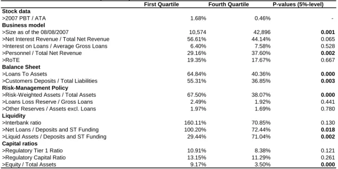
subsequent capital actions (dividends). They therefore better reflect total value created or destroyed for shareholders. Operational performance is described by the Pre-Tax Profit to Average Tangible Assets (PBT / ATA) ratio. The reason for using average assets is that banks assets vary significantly across the year. Taking a punctual figure would also lead to a biased view of operational performance. We also attend to correct this imperfection by taking an average number. The first advantage of this metric is that it is not artificially inflated by the gearing effect (which is the case for RoTE). Moreover, it is not impacted by local tax regulations and one-off post-tax items. By taking into account the whole balance sheet, it provides with an acceptable approximation of what has been necessary to generate earnings. However, the PBT / ATA ratio does not take directly into account assets risks nor off-balance sheet items. We compute our PBT / ATA ratio using pre-tax profits, intangibles and total assets reported in Bankscope. We provide a description of the sample performance features in table 1.

1.2. Business model choices

We focus on five variables which reflect the business model choices:

- Size. As a metric for size, we use market capitalization at the end of 7 August 2007 and 9 March 2009 trading days. The underlying hypothesis is that the crisis hits small institutions more painfully than larger ones as the latter should offer better business and geographical diversification, benefit from better risk-management devices and enjoy easier access to funding resources.

- Net Interest Revenue to Net Revenue ratio. We compute this ratio from the data available in Bankscope for net interest revenue and net revenue. Our hypothesis is that banks which were more exposed to non-interest-earning activities underperformed their peers because of heavy losses in their trading books and the general fallback of cyclical activities (brokerage, advisory, households’ consumption etc.). We expect an inverted relationship during the recovery phase.

- Interest Income on Loans to Gross Loans ratio. This metric is directly sourced from Bankscope. We expect banks which received higher interest earnings before the crisis to have been more impacted by the downturn than other institutions, as high interests should correspond to riskier credit lines.

- Personnel expenses to Net Revenue ratio. We calculate this metric thanks to personnel expenses and net revenue provided in Bankscope. Generous compensation practices are expected to have encouraged risk-taking, which should translate into underperformance during the crisis.

- Return on Tangible Equity (RoTE). We compute this metric using net income, book value and intangible obtained from Bankscope. Banks with high 2006 RoTE should have underperformed their peers during the crisis because a high RoTE can be obtained by minimizing loan losses provision and by dangerously reducing the weight of equity within the balance sheet. The impact of 2008 RoTE is more ambiguous as banks with extraordinary low (negative) RoTE may have benefited from a stronger recovery effect both from a market and operational point of view.

1.3. Balance-sheet structure

We analyze here two variables which are important characteristics of banks balance sheet structure:

- Loans to Total Assets ratio. We take the required figures directly from Bankscope. We expect banks with more loans in the asset side of their balance-sheet to have outperformed

(18)

their peers during the crisis. Loans beget more stable revenue streams than those issued from non-interest earning activities, even though they are likely to drive a rise in loan losses provisions. The recovery phase should be characterized by an inverted relationship between Loans to Assets ratio and performance.

- Deposits to Total Liabilities ratio. We compute this ratio based on customers’ deposits and balance sheet size recorded in Bankscope. Banks relying more heavily on deposits for their short-term funding depend less on the wholesale market. They should therefore have less suffered than their peers from the complete freeze of the interbank lending market and also display relative outperformance during the core phases of the financial crisis.

1.4. Risk-management policy

In this section, we first challenge the link between a bank provision policy and its relative performance during the crisis. Our hypothesis is that conservatism in provisioning choices has led to outperformance during the crisis because it provides with reserves that can be reversed to smooth the effect of gross loan losses provision that can only expand in a depressed economic environment. Moreover, a higher level of provisions could be synonym for a better apprehension of risk by banks internal control departments. We use the Loans Loss Reserve to Gross Loans ratio and the Other Reserves to Assets excluding Loans to assess our hypothesis. The first metric is directly available in Bankscope. The second one is computed using total reserves, total assets, loan loss reserves and net loans available in Bankscope.

We then investigate the relationship between performance and Risk-Weighted Assets (RWA) to Total Assets ratio. We compute this ratio using RWA including floor and cap hedging tools and total assets provided by Bankscope. We try therefore to build a metric able to reflect the underlying risk of a bank assets and activities. RWA to Total Assets is an imperfect estimate of balance sheet assets risks because RWA include off-balance sheet items but it is nevertheless interesting to investigate. The nature of the relationship (if any) between this indicator and performance is uncertain as one could consider that conservative banks would tend to major their RWA, leading to a higher RWA to Total Assets ratio, whereas more aggressive banks would minor it. In that case, there would be a direct relationship between performance and the level of the ratio. On the other hand, one could think that RWA fairly translate banking institutions’ losses exposure and that small RWA to Total Assets ratio should be synonym for relative outperformance during the crisis.

1.5. Liquidity Characteristics

We expect banks offering good liquidity profile to outperform their peers as banks whose liabilities contain a significant part of deposits and equity should be less dependent on the interbank lending market for their refinancing. The share of liquid assets is also important as the greater it is, the lower should be the negative impact in case some of them become illiquid. They may also be used as collaterals to secure access to short-term resources. To capture the level of liquidity of a bank balance-sheet, we rely on three variables, all directly taken from Bankscope:

- The Interbank ratio. This ratio is obtained by dividing the total amount of money lent to other banks by the total amount of money borrowed from other banking institutions. A bank with an interbank ratio below 1 is also a net liquidity borrower on the interbank lending market. Our hypothesis is that low interbank ratios go along with the least enviable performances during the crisis.

(19)

- Net Loans to Short-term (ST) Funding and Deposits ratio. This indicator measures the discrepancy between loans granted (post impairment) and short-term resources. Our hypothesis is that the more this ratio is above 1, the riskier is the related bank as the expansion of its loans portfolio has been found by unstable short-term resources. This should lead to measurable underperformance against peers.

- Liquid Assets to Short-term Funding and Deposits ratio. This ratio captures the ability of a bank, in an extreme situation, to reimburse its short-term resources with its immediately sellable assets. The lower this ratio is, the more the related bank is at risk. We expect banks displaying low Liquid Asset to Short-term Funding and Deposits ratio to have underperformed their comparables during the crisis.

1.6. Regulatory capital requirements

The hypothesis we want to challenge in this section is that the best capitalized banks were the least impacted by the crisis as they had enough equity to absorb their losses without needing recapitalization or facing bankruptcy risk. We also intend to understand whether the qualitative properties of banks capital compared to risk-adjusted measure of their assets (RWA) had any influence on their performance. To assess banks qualitative and quantitative capitalization, we use three classical metrics directly streamed from Bankscope.

- Regulatory Tier 1 Capital ratio whose denominator is RWA. - Regulatory Capital ratio whose denominator is also RWA. - Equity to Total Assets (Leverage) ratio.

2. Our data analysis methodology

In order to identify the characteristics of the best-and-worst performers, we first sort the banks of our sample in different quartiles according to their market and operational performance over the periods of time we have previously determined. Then we compute the arithmetic average of the first and fourth quartile for each business-related indicator we want to test. To assess the consistency of these results, we run tests of equality of means assuming equal variances. We only retain variables for which we obtain p-values below 0.050 at the 5%-level.

In a second part of our work, we run several regressions to assess the robustness of the findings of the first part. Some variables are indeed correlated and we therefore have to correct multi-co-linearity problems. We first implement simple regressions (called “Individual” in tables 11 and 12) on each of our criteria to measure their individual contribution to banks performance. We also run a multiple regression (“Global”) on all our variables to have an idea of their explanatory power. We then restrict ourselves to the indicators we had identified in our tests of equality of means in regression called “Test of

means”. Finally, we use a Fisher backward selection process10

to find out the multiple

regression (“Fisher BS”) which returns the best R2

and whose factors are individually significant (with p-values below 0.050 at the 5%-level). Through this process, we are able to identify the core determinants of banks market and operational performance during the crisis.

In a last part, to check the robustness of the results we obtain using the previously-described approach, we implement a Fisher forward selection process. We compute two regressions per period: the first one (“Fisher FS”) is the pure result of the Fisher forward selection. The second one (“Best n+1”) is obtained by adding to the variables returned by the

10

In a Fisher backward selection process with n factors, the first regression includes the n variables. The one which returns the highest p-value is withdrawn from the set and a new regression is computed with the remaining n-1 variables. The same process is repeated until it remains only individually-significant factors.

(20)

Fisher forward selection11 the next least insignificant factor. During all our regression work, we cautiously monitor the significance of the Fisher value of the whole multiple regression.

All our computations have been led using Excel which only manages 16 explicative variables within multiple regressions. This explains why we have restricted ourselves to the indicators described in the previous part. In the following lines, all mentioned p-values are computed at the 5%-confidence level unless otherwise specified.

3. Market performance of banks over the crisis and recovery phase

This section exposes the characteristics of the best and worst market performing banks of our sample during the financial crisis. We then run various simple and multiple regressions to assess the explanatory power of the determinants previously identified. Stock returns from

the 8th August 2007 to the 12th September 2008 and from the 12th September 2008 to the 9th

March 2009 are regressed against business characteristics of fiscal year 2006. Stock returns

from the 9th March 2009 to the end of 2009 are regressed against business characteristics of

fiscal year 2008. By proceeding this way, we are able to determine whether the drivers of banks performance have changed between the core-crisis periods and the recovery phase. We can also understand what is valuable to the market at these different periods.

3.1. Main drivers of market performance

The results of the study we led on the characteristics of worst and best performing banks are displayed in tables 5 (first period), 6 (second period) and 7 (third period).

3.1.1. Pre-Lehman phase of the crisis: European banks indiscriminately sold by the market

Over the first period, the average share-price of our best-performer quartile declined by 22.51% versus 56.24% for the worst performers. A striking result is that there is no statistically-significant difference between the characteristics of best-and-worst performers over the first period of the crisis. This being despite absolute differences superior to 25% between means of best-and-worst performing quartiles on Size (€31,674bn vs. €24,482bn), provision metrics, Interbank ratio (98.02% vs. 67.82%) and Equity to Total Assets (6.64% vs. 5.11%). This is a destabilizing finding which suggest in the early stages of the crisis, investors sold the European banking sector as a whole without looking cautiously at individual characteristics.

At the beginning of the crisis, the extent of the potential losses caused by rotten credit

derivatives was not precisely known (see, for instance, le Monde of the 9 August 200712

which mentions potential losses of €100bn, more than twenty times below the actual figures). Neither were the most exposed institutions as securitization has spread risk from originators to most of market participants. This might explain why the metric for which we find the smallest p-value (0.068) is the Loan to Total Assets ratio. Given the lack of visibility on the extent of the downturn, investors might have uniquely focused on the level of capitalization. The lower it is, the more a bank is at risk to see a large part of its equity disappear to compensate losses stemming from large assets write-offs. It also raises the risk of a

11

In a Fisher forward selection process, individual regressions are computed for the n factors that have to be analyzed. The one which return the smallest p-value is isolated. N-1 multiple regressions are then computed using the identified factor and the remaining n-1 variables. The one which returns the lowest value is also isolated. The process is repeated until it becomes to find an additional variable with a p-value below 0.050.

12

(21)

scale, massively-dilutive capital increases. Moreover, as it is a synonym for higher bankruptcy risk, it jeopardizes access to reasonable short-term financing conditions in a distressed market environment.

3.1.2. Core phase of the crisis: Investors privileged the most traditional business models

Over the second period, the average share price of our best-performer quartile was -34.07% versus a severe -83.56% for the fourth quartile. The best performing banks were first

the ones which had the smallest market capitalization before the burst of the crisis in August 2007. One average, first-quartile banks had a market capitalization of €6,153bn, four times lower than the average market capitalization of fourth-quartile institutions. The second characteristic of the best-performing banks was a Net Interest Revenue to Total Net Revenue of 61.56% in 2006, compared to an average ratio of 52.67% for worst-in-class players. The latter had also posted an average RoTE of 23.39% in 2006, strikingly better than the average 15.43% average 2006 RoTE delivered by banks of the first quartile. Regarding balance sheet characteristics, investors spared banks with high Loans to Assets ratios (72.33% for the first quartile vs. 53.56% for the worst performing banks). On risk-management policy, first-quartile banks reported an average RWA to Total Assets ratio of 70.89% whereas it only amounted to 51.10% for the fourth-quartile. Best-performers had also booked higher risk provisions than their peers. On liquidity, institutions with higher Net Loans to Deposits and ST funding ratios enjoyed better resilience. The last feature of the best performers was a lower Liquid Assets to Deposits and ST Funding ratio of 22.30% versus 38.25% among worst underperformers.

These findings tend to prove that the panic movement that hurt the European banking sector has not been so blind and absurd than it is often said to have been. On the contrary, investors mostly sold large institutions which had the most moved apart from traditional lending activities and had been more likely to develop risky businesses. This move is more likely to have been implemented by big institutions which had the necessary means to develop large capital market divisions. Moreover, given the fixed-cost structure of banks, large players can benefit from material economies of scale especially in the IT and compliance expenses that are required to run large capital markets businesses. Among our findings, the most difficult to interpret are the results on the RWA to Total Assets ratio and on liquidity. Our hypothesis is that large banks, which delivered the worst performance over the period, are more likely to have adopted the Internal-Ratings Based (IRB) approach, which gives banks enhanced freedom when computing their RWA. On the contrary, smaller institutions are more likely to have followed the Standardized Approach (SA) where there is virtually no scope for individual interpretation of the regulatory framework. As a consequence, it may have been easier for large banks to underestimate their RWA by using proprietary risk-monitoring models, leading to lower RWA to Total Assets ratios. Our results on liquidity are also disturbing because they show that banks which apparently had the most risky profiles eventually outperformed their peers. Our best explanation on Net Loans to Deposits and ST – funding ratio is that small players whose businesses relied mostly on loan granting mechanically have high ratios. A possible explanation of our result on Liquid Assets / Deposits and ST Fund ratio is first that a material proportion of liquid assets booked by large players in 2006 had turned illiquid in 2008-2009, fuelling stocks decline. It might also be because the traditional interbank money market had stopped and had been compensated by the ECB. As the latter accepted almost all assets as collateral in the refinancing process, their liquidity properties may had lost some of their importance.

Over the two core-crisis periods, capitalization characteristics have not appeared as significant differences between best-and-worst performers. This may be due to the various

(22)

State interventions to recapitalize or grant loans to banks. This behavior of European States made banks bankruptcy more hypothetical, reducing the importance for investors to monitor the ability of 2006 equity to absorb subsequent losses. Another interesting learning from our results is that interbank ratios at end-2006 are not associated with significant differences in banks performance during the crisis. This may be explained by the almost-complete freeze of the interbank lending market over the period. As central banks took in charge the vast majority of commercial banks funding needs (see Trichet 2010), investors may not have been interested in the level of reliance on the wholesale funding market as reported by the interbank ratio at end-2006.

3.1.3. Recovery period: Investors’ preference turned back to risky business models

Over the third period, the 61 banks we have studied recovered by 127.48% on average. The first quartile performance reached 255.49% and was therefore almost ten times higher than the 26.37% average recovery of the fourth quartile. Primary beneficiaries of the recovery were large institutions (average size of €23.5bn versus 3.5bn for the fourth quartile), with reduced weight of loans among assets (Loans to Assets ratios of 55.12% versus 74.78% for the fourth quartile). The average Customers Deposits to Total Liabilities ratio of the first-quartile banks was 35.23%, well below the 48.01% mean ratio posted by the fourth first-quartile. Moving to risk-management policy characteristics, the slowest recovers had RWA to Total assets ratio of 69.50% for the worst-performing banks and versus 48.04% for the top performers. Moreover, they reported lower Loans Loss Reserves as a percentage of Gross Loans. Liquidity was also of importance during the recovery phase as best-performers posted interbank ratios of 50.89%, twice as small as the average of the fourth quartile. Best institutions also had higher Liquid Assets to Deposits and Short-term funding ratios, with an average number of 34.99% for the first quartile against 17.58% for the fourth quartile. Finally, the fastest-recovering institutions were the most leverage, with an average Equity to Total Assets ratio of 4.56% below the average 6.62% of the worst-performers.

It therefore appears that during the recovery phase, investors preferred companies whose characteristics were quite the opposite of second-period best performers. The main beneficiaries of the recovery were indeed large companies following the riskiest business models implying reduced reliance on equity, enhanced use of wholesale funding, and a limited weight of loans in the assets side of the balance sheet. This can be explained by the fact that these institutions were more likely to benefit from the market post-crisis rally, from the large number of refinancing operations and from the upturn in advisory and advisory-related activities. Our findings on the Liquid Assets to Deposits and Short-term funding ratio suggest that a key concern of investors in the post-core crisis environment has been on the ability of banks to manage liquidity risk and to keep a sufficient amount of liquid assets compared to their short-term commitments.

3.2. Results of the various multiple regressions conducted

The results of our findings are displayed in table 11. For each period of time, we computed four regressions following principles described in section 2.

3.2.1. First period: possible role of size and capitalization unveiled

Over the first period, the individual regressions we led returned no significant result.

The most significant variable was once again Equity to Total Assets (positive coefficient, R2

(23)

proved to be globally insignificant. We did not compute our “Test of means” regression over the first period as we had not identified any significant difference between worst-and-best performers. The Fisher backward selection process returned significant findings, using both Size and Equity to Total Assets. The two parameters were associated with positive

coefficients and significant p-values. The overall regression reached a R2 of 0.123 and the

p-value of the F-test was 0.022. This tends to confirm that banks with a relatively high level of book equity compared to the size of their balance sheets were preferred by investors always concerned about bankruptcy and capital increase risk. The economic meaning of the size factor is more difficult to explain. A first hypothesis is that investors tended to prefer large banks because of a “too big to fail” effect, which would highlight a moral hazard phenomenon. One could also believe that large European institutions ran sufficiently diversified activities to mitigate particularly tough conditions in certain local markets. This might be true at least for certain institutions like HSBC or Standard Chartered which have important activities in Asia. There is no clear way to choose between these two possibilities.

This being said, the results of this first set of regressions tend to back the conclusions of our test of equality of means showing that investors sold the banking sector for reasons that are not captured by the criteria we studied.

3.2.2. Second period: key role of the loans to assets ratio confirmed, role of asset liquidity identified

Over the second period, individual regressions highlighted the individual significance of the banks characteristics we had identified in section 3.1 for worst-and-best performers. Coefficient signs confirmed the sense of the relationships previously established. Interestingly, Loans to Assets and Net Loans / Deposits and ST Funding ratios were still

significant in our “Global” regression which also returns a R2

of 0.406 and an overall p-value of 0.050. However, the sign of the relationship between Liquid Assets / Deposits and ST Funding ratio and market performance inverted and turned positive, which seems more consistent with economic intuition. We found similar results in our “Test of means”

regression. Suppressing ten explanatory variables led to a global R2 of 0.317 and improved

the significance of our regression with a p-value of 0.004. The two factors previously mentioned remained significant. Finally, the Fisher backward selection led us to a regression including solely Loans to Assets and Liquid Assets / Deposits and ST Funding ratios. It

returned a high R2 of 0.282 for a p-value of 0.000. The individual p-values of these two

factors were both below 0.005, denoting a high significance of our findings.

These findings tend to prove that the main drivers of banks during the core-phase of the crisis were the proportion of loans within the balance sheet and the ability of liquid assets to cover short-term commitments. Their economic meaning is fairly robust as banks that have remained faithful to a conservative business model have mechanically been protected against the decline of non-interest revenue and financial markets collapse. This has translated into relative outperformance against peers. This result also allows to understand observations made in section 3.1 as a high proportion of loans in the balance sheet is logically associated with higher contribution of net-interest revenue to total net revenue, lower RoTE and smaller institutions which had not developed large-scale risky capital market activities. Loans to Assets ratio also accounts for the relationship between Net Loans / Deposits and ST Funding highlighted both in section 3.1 and in individual regressions.

The observation we had made on Liquid Assets to Deposits and ST Funding ratio in section 3.1 was also probably biased by the distribution of our first and fourth quartiles. It indeed appears more intuitive to consider that banks whose liquid assets better matched

The performance of banks during the financial crisis

The performance of banks during the financial crisis

Table of Contents