Asymptotic methods in stochastic control and applications in finance

(1)

Université Paris Diderot

École Doctorale de Science Mathématiques de Paris Centre

Laboratoire de Probabilités et Modèles Aléatoires

Thèse de doctorat

Discipline : Mathématiques appliquées

présentée par

Jiatu Cai

Méthodes asymptotiques en contrôle stochastique et

applications à la finance

Asymptotic methods in stochastic control and

applications in finance

co-dirigée par Mathieu Rosenbaum et Peter Tankov

Soutenue le 25 Mars 2016 devant le jury composé de :

Emmanuel Gobet

Ecole Polytechnique

rapporteur

Jean Jacod

Université Pierre et Marie Curie examinateur

Johannes Muhle-Karbe University of Michigan

rapporteur

Huyên Pham

Université Paris Diderot

examinateur

Mathieu Rosenbaum

Université Pierre et Marie Curie directeur

Mete Soner

ETH Zürich

examinateur

Peter Tankov

Université Paris Diderot

directeur

(2)

(3)

Résumé

Dans cette thèse, nous étudions plusieurs problèmes de mathématiques financières liés à la pré-sence d’imperfections sur les marchés. Notre approche principale pour leur résolution est l’uti-lisation d’un cadre asymptotique pertinent dans lequel nous parvenons à obtenir des solutions approchées explicites pour les problèmes de contrôle associés.

Dans la première partie de cette thèse, nous nous intéressons à l’évaluation et la couverture des options européennes. Nous considérons tout d’abord la problématique de l’optimisation des dates de rebalancement d’une couverture à temps discret en présence d’une tendance dans la dynamique du sous-jacent. Nous montrons que dans cette situation, il est possible de générer un rendement positif tout en couvrant l’option et nous décrivons une stratégie de rebalancement asymptotiquement optimale pour un critère de type moyenne-variance. Ensuite, nous proposons un cadre asymptotique pour la gestion des options européennes en présence de coûts de tran-saction proportionnels. En s’inspirant des travaux de Leland, nous développons une méthode alternative de construction de portefeuilles de réplication permettant de minimiser les erreurs de couverture.

La seconde partie de ce manuscrit est dédiée à la question du suivi d’une cible stochastique. L’objectif de l’agent est de rester proche de cette cible tout en minimisant le coût de suivi. Dans une asymptotique de coûts petits, nous démontrons l’existence d’une borne inférieure pour la fonction valeur associée à ce problème d’optimisation. Cette borne est interprétée en terme du contrôle ergodique du mouvement brownien. Nous fournissons également de nombreux exemples pour lesquels la borne inférieure est explicite et atteinte par une stratégie que nous décrivons. Dans la dernière partie de cette thèse, nous considérons le problème de consommation et inves-tissement en présence de taxes sur le rendement des capitaux. Nous obtenons tout d’abord un développement asymptotique de la fonction valeur associée que nous interprétons de manière probabiliste. Puis, dans le cas d’un marché avec changements de régime et pour un investisseur dont l’utilité est du type Epstein-Zin, nous résolvons explicitement le problème en décrivant une stratégie de consommation-investissement optimale. Enfin, nous étudions l’impact joint de coûts de transaction et de taxes sur le rendement des capitaux. Nous établissons dans ce cadre un système d’équations avec termes correcteurs permettant d’unifier les résultats de [ST13] et [CD13].

Mots-clefs

Couverture discrète, théorèmes limites, temps d’arrêt, optimalité asymptotique, coût de tran-sactions, contrôle linéaire-quadratique, stratégie de Leland, variance conditionnelle, contrôle singulier, théorème limite central, mesure d’occupation, borne inférieure asymptotique, contrôle impulsionnelle, contrôle moyen en temps, programmation linéaire, problème de martingale, maxi-misation d’utilité, discrétisation des intégrales stochastiques, coût illiquidité, impact de marché temporaire, taxe de rendement des capitaux, utilité récursive, Epstein-Zin, homogénéisation.

(4)

(5)

Abstract

In this thesis, we study several mathematical finance problems related to the presence of market imperfections. Our main approach for solving them is to establish a relevant asymptotic frame-work in which explicit approximate solutions can be obtained for the associated control problems. In the first part of this thesis, we are interested in the pricing and hedging of European options. We first consider the question of determining the optimal rebalancing dates for a replicating portfolio in the presence of a drift in the underlying dynamics. We show that in this situation, it is possible to generate positive returns while hedging the option and describe a rebalancing strategy which is asymptotically optimal for a mean-variance type criterion. Then we propose an asymptotic framework for options risk management under proportional transaction costs. Ins-pired by Leland’s approach, we develop an alternative way to build hedging portfolios enabling us to minimize hedging errors.

The second part of this manuscript is devoted to the issue of tracking a stochastic target. The agent aims at staying close to the target while minimizing tracking efforts. In a small costs asymptotics, we establish a lower bound for the value function associated to this optimization problem. This bound is interpreted in term of ergodic control of Brownian motion. We also provide numerous examples for which the lower bound is explicit and attained by a strategy that we describe.

In the last part of this thesis, we focus on the problem of consumption-investment with capital gains taxes. We first obtain an asymptotic expansion for the associated value function that we interpret in a probabilistic way. Then, in the case of a market with regime-switching and for an investor with recursive utility of Epstein-Zin type, we solve the problem explicitly by providing a closed-form consumption-investment strategy. Finally, we study the joint impact of transaction costs and capital gains taxes. We provide a system of corrector equations which enables us to unify the results in [ST13] and [CD13].

Keywords

Discrete hedging, limit theorems, stopping times, asymptotic optimality, transaction costs, linear-quadratic control, Leland strategy, conditional variance, singular control, central limit theo-rem,occupation measure, asymptotic lower bound, impulse control, time-average control, linear programming, martingale problem, utility maximization, discretization of stochastic integrals, illiquidity cost, temporary market impact, capital gains taxes, recursive utility, Epstein-Zin, homogenization.

(6)

(7)

6 Joint impact of capital gains taxes and transaction costs 195 6.1 Main result . . . 196 6.1.1 HJB equation . . . 196 6.1.2 Benchmark model . . . 196 6.1.3 Asymptotic expansion . . . 197 6.2 Probabilistic interpretation . . . 198 6.3 Homothetic case . . . 200 6.4 Asymptotic development . . . 201 6.4.1 Fast variables . . . 201 6.4.2 Corrector equations . . . 203 Bibliography 207

(10)

(11)

Introduction

This thesis is devoted to the study of three different problems in mathematical finance, which involve various important market features such as time discretization, transaction costs and capital gains taxes. Due to the presence of these market features, the optimal strategies de-duced from most of the existing financial models cannot be implemented in practice. Therefore more complex models and advanced theoretical tools have been developed in order to deal with these market imperfections. However, the resulting stochastic control problems often become intractable. While it is possible to obtain numerical solutions in some cases, the required com-putational effort in reality is usually prohibitively large. In this thesis, we aim at proposing an asymptotic framework for the associated stochastic control problems, providing explicit and fea-sible optimal strategies. We focus both on the theoretical investigation of the related stochastic control methods, and on the economic analysis of the impact of market frictions.

In the first part, we study the pricing and hedging of option when taking into account discrete rebalancing and transaction costs.

In Chapter 1, we consider the hedging error of a derivative due to discrete trading. It turns out that, in the presence of a drift in the dynamics of the underlying asset, the trader can actually benefit from market trend. We suppose that the trader wishes to find rebalancing times for the hedging portfolio which enable him to keep the discretization error small while taking advantage of market tendency. Assuming that the portfolio is readjusted at high frequency, we introduce an asymptotic framework in order to derive optimal discretization strategies. More precisely, we formulate the optimization problem in terms of an asymptotic expectation-error criterion. In this setting, the optimal rebalancing times are given by the hitting times of two barriers whose values can be obtained by solving a linear-quadratic optimal control problem. In specific contexts such as in the Black-Scholes model, explicit expressions for the optimal rebalancing times can be derived.

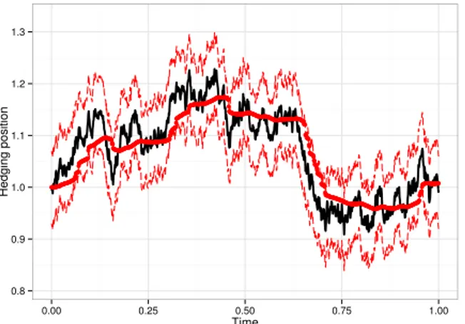
In Chapter 2, we study the dynamic hedging of a European option under a general local volatility model with small proportional transaction costs. Extending the idea of Leland, which consists in modifying the volatility in the pricing PDE in order to compensate the costs incurred by discrete rebalancing, we consider instead a continuous version (with finite variation) of Leland’s strategy that asymptotically replicates the payoff. In the limit of small proportional costs, an associated central limit theorem for hedging error is proved. The asymptotic variance is minimized by an explicit replication strategy. Depending on the transaction costs and the gamma of the option, the optimal replication strategy is given by either an absolutely continuous process or a singular process based on two barriers around a benchmark position. Numerical simulations demonstrate a significant improvement of our strategies over Leland’s strategy in terms of conditional vari-ance of the hedging error.

In the second part, we consider tracking problems which arise from the study of trading strategies under various market frictions and discretization effects. The aim is to minimize both deviation from the target and tracking efforts.

(12)

In Chapter 3, we propose an asymptotic framework and establish the existence of asymptotic lower bounds for the value functions of the corresponding control problems. These lower bounds can be related to the time-average control problem of Brownian motion. A key step is the use of a linear programming characterization of the lower bounds. Our probabilistic approach enables us to treat (the combination of) different control types such as (absolutely continuous) regular control, singular control and impulse control. Moreover, the lower bound are shown to hold pathwise. A comprehensive list of examples with closed-form solutions for the lower bounds is also provided.

In Chapter 4, we focus on strategies of feedback form for the problem of tracking and study their performance under our asymptotic framework. Depending only on the current state of the system, these strategies maintain the deviation from the target inside a time-varying domain. Although the dynamics of the target is non-Markovian, it turns out that they asymptotically attain the lower bounds previously established for a large list of examples. We apply our results to the analysis of discretization errors of stochastic integrals and impact of market frictions on portfolio management.

In the third part of this thesis, we perform asymptotic analysis for the problem of consumption-investment optimization with capital gains taxes.

In Chapter 5, we study the optimal consumption and portfolio decisions in the presence of cap-ital gains tax and stochastic investment opportunity. The option to defer taxation of capcap-ital gain gives rise to an optimal investment strategy consisting of buy and sell boundaries around the tax-deflated Merton line. In a bull-bear switching market, the optimal investment strategy is affected by the investment opportunity in the other regime. Consequently, there is a cross-regime smoothing effect on the value of the deferral option. Moreover, cross-regime switching has a greater impact under the bear regime and in the region of high capital gains. Depending on the level of capital gains, a sudden change of economic condition might not lead to an instanta-neous jump in the optimal portfolio allocation. In contrast, for an investor with recursive utility, the EIS of the investor determines the optimal consumption rate but has little impact on the optimal investment strategy. Our asymptotic analysis is supported not only by numerical res-olution of the corresponding PDEs but also by an underlying two time scales probabilistic model. In Chapter 6, we are interested in the joint impact of capital gains taxes and transaction costs. Guided by the local probability model developed in the previous chapter, we develop a new system of corrector equations, unifying previous results on capital gains taxes and transaction costs via homogenization technique. In particular, we find that the presence of capital gains taxes has an equivalent effect of increasing selling costs for the non-transaction zone.

(13)

Part I : Option pricing and hedging

1.1 Discrete hedging with directional views

In order to manage the risks inherent to the derivatives they buy and sell, practitioners use continuous time stochastic models to compute their prices and hedging portfolios. In the simplest cases, notably in that of the so-called delta hedging strategy, the hedging portfolio obtained from the model is a time-varying self-financed combination of cash and the underlying. We denote the price at time t of the underlying asset by Yt and assume it to be a one-dimensional semi-martingale. Hence, in such situations, the outputs of the model are the price of the option together with the number of shares in the underlying asset to be held in the hedging portfolio at any time t, denoted by Xt. The proportion invested in cash is then deduced from the self-financing property. Therefore, assuming zero interest rates, the theoretical value of the model-based hedging portfolio at the maturity of the option T is given by

⁄ T

0 XtdYt.

Typically, the process Xtderived from the model is a continuously varying semi-martingale, re-quiring continuous trading to be implemented in practice. This is of course physically impossible and would be anyway irrelevant because of the costs induced by microstructure effects. Hence practitioners do not use the strategy Xt, but rather a discretized version of it. This means that the hedging portfolio is only rebalanced a finite number of times and is held constant between these times. Let us denote by (·n

j )jØ0 an increasing sequence of rebalancing times over [0, T ].

With respect to the target portfolio obtained by continuous rebalancing, the hedging error due to discrete trading Zn T is therefore given by Z_Tn = +Œ ÿ j=0 X·n j(Y·jn+1·T ≠ Y·jn·T) ≠ ⁄ T 0 XtdYt.

Why market trends matter ?

When X and Y are Itˆo processes, the case of equidistant rebalancing dates ·n

j = jT/n has been investigated in [BKL00, HM05, Roo80]. In these works, the following convergence in law is proved: Ô nZ_Tn_≠_æL Û T 2 ⁄ T 0 ‡ X t ‡tYdBt, (1.1)

where ‡X and ‡Y are the volatilities of X and Y and B is a Brownian motion independent of the other quantities.

This asymptotic approach has also been recently used in [Fuk11c, RR10, GL14a, Lan13], where the rebalancing times are random stopping times. More precisely, for a given parameter n driving the asymptotic, one considers an increasing sequence of stopping times

0 = ·n

0 < ·1n< . . . < ·jn< . . . with Nn

t := max{j Ø 0; ·jnÆ t} < Œ almost surely for any t Ø 0. When E[(X·n j+1≠ X·jn) 4_|F ·n j] E[(X·n j+1≠ X·jn) 2_|F ·n j] = Á2 na2·n j + op(Á 2 n), E[(X·n j+1≠ X·jn) 3_|F ·n j] E[(X·n j+1≠ X·jn) 2_|F ·n j] = ≠Áns·n j + op(Án)

(14)

for a sequence Án æ 0 and left continuous adapted processes a and s, it is shown in [Fuk11c] that Á≠1 n Zn converges weakly to 1 3 ⁄ _· 0 stdYt+ 1 Ô6 ⁄ _· 0 ! a2_t ≠2₃s2_t"1/2‡Y_t dBt, (1.2) where B is a Brownian motion independent of all the other quantities.

One can remark a crucial difference between the deterministic discretization schemes associated to (1.1) and the random stopping times case leading to (1.2). For deterministic dates, the discretization error asymptotically behaves as a stochastic integral with respect to Brownian motion. Therefore, it is centered. In the case of random discretization dates, one may obtain a “biased” asymptotic hedging error because of the presence of the term

⁄ T

0 stdYt.

Hence, if s does not vanish and Y has non zero drift, the asymptotic hedging error is no longer centered.

An asymptotic linear-quadratic criterion

A natural question is to determine the efficient frontier for the first and second moments of hedging errors and to find stopping times ·n

j which attain the efficient frontier. More precisely, we are interested in inf (·n j) ! ≠ Á≠1n E[ZTn], Á≠2n E[(ZTn)2] " , (1.3)

as Án æ 0, meaning that the hedging frequency is high and the hedging error should be small. Our main contribution in Chapter 1 is the following result.

Main Result 1. The efficient frontier of (1.3) can be explicitly determined from the solution

of the following optimal control problem

inf (st) ≠E[Z ú s,T] + ⁄E Ë (Zú s,T)2+ 1 2 ⁄ T 0 s 2 t(‡Yt )2dt È , (1.4) where Z_s,Tú = ⁄ T 0 stdYt.

Moreover, given an optimal strategy sú

t for (1.4), one can construct explicitly two barriers lút and

lú_t such that the sequence of rebalancing dates (·_jn,ú) defined by

·_jn,₊₁ú = infÓt > ·_jn,ú : Xtœ (X/ ·_jn,ú≠ Ánlút, X·_jn,ú+ Ánlút)

Ô · T

attains asymptotically the efficient frontier of (1.3).

Comparing to the classical continuous-time portfolio selection problem without hedging con-straint and discrete rebalancing (see [ZL00])

inf (st) ≠E[Z ú s,T] + ⁄E #_(Z_ú s,T)2 $ ,

we note that the discrete nature of the hedging strategy introduces an extra uncertainty on the final hedging error, which is approximately quantified in (1.4) by

EË1₂⁄ T 0 s 2 t(‡tY)2dt È ,

(15)

as Án tends to zero.

1.2 Option replication with modified volatility

In Chapter 2, we develop a framework for option pricing and replication under proportional transaction costs. As we have seen in the previous section, without transaction costs the hedging error with respect to the target portfolio tends to zero as the rebalancing dates become more frequent. However, transaction costs increase as the rebalancing intervals decrease. Therefore, when pricing and hedging derivatives, one should include transaction costs. Inspired by the work of [Lel85], our approach has the following advantages :

1. The strategy replicates the option payoff under transaction costs, with an error whose distribution is explicitly determined in the limit of small costs.

2. We find explicit strategies minimizing the conditional variance of hedging errors.

In order to explain our framework and state the main results, we begin by a brief review of Leland’s strategy in the Black-Scholes framework.

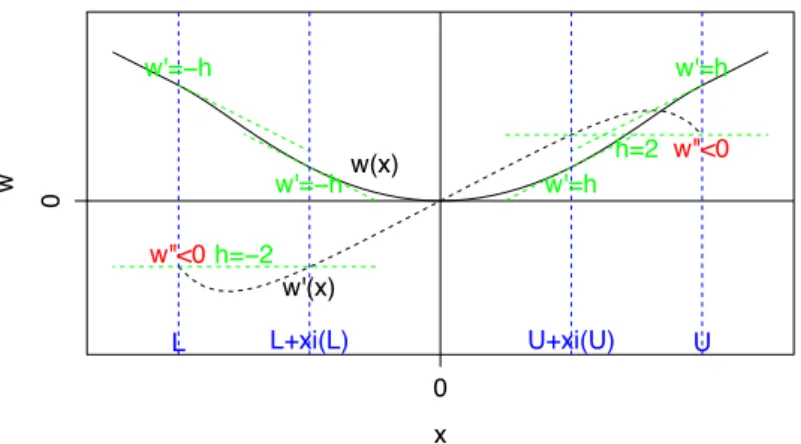
Leland’s idea has two ingredients. The first is to find a good benchmark strategy by an en-largement of volatility, yielding certain surplus in the absence of transaction costs . Let p– _{be a} solution of the partial differential equation

ˆtp–(s, t) + 1₂ 3 1 + 2 – 4 ‡2s2ˆ_s2p–(s, t) = 0, p–(s, T ) = f(s), (1.5)

where f(s) = (s ≠ K)+ _{is the payoff of a European call option, T is the maturity of the option,}

‡ is the volatility of Black-Scholes model. Here, – is an arbitrary positive constant that controls

the enlargement of volatility, which should be determined by market supply-demand equilibrium. By Itˆo’s formula, we have

f(ST) = –0 + ⁄ T 0 X – udSu≠ 1 – ⁄ T 0 – udÈSÍu, where – t = p–(St, t), Xt– = ˆsp–(St, t), –t = ˆs2p–(St, t). (1.6) This means that, without transaction costs and assuming zero interest rates, the self-financing strategy X– _{with initial capital} –

0 super-hedges the payoff f(ST) with surplus 1 – ⁄ T 0 – tdÈSÍtØ 0, (1.7)

where –_{Ø 0 follows from the convexity of the payoff f.}

The second step of Leland’s strategy is to construct a good approximation of the benchmark

X– _{by a strategy with finite transaction cost so that the incurred costs are compensated by the} surplus. Assume that the trader has to pay Ÿ| X| to buy or sell X shares of stocks, where

Ÿ is a positive constant representing the proportional transaction costs. Leland considers an

equidistant discretization of X– _{defined by}

X_t–,Ÿ = X_jh–, t_{œ (jh, (j + 1)h], j = 0, 1, 2, . . . ,} (1.8)

with h > 0 the interval of rebalancing. Set the initial capital –,Ÿ

0≠, that is the price of the option,

to be

–,Ÿ

(16)

The second term is to compensate the transaction cost at the inception. The associated wealth process –,Ÿ _{under transaction costs is then}

–,Ÿ t = –0 + ⁄ t 0 X –,Ÿ u dSu≠ Ÿ ÿ 0<uÆt Su| Xu–,Ÿ|. (1.9) By choosing h= 2 ﬁ Ÿ2–2 ‡2 , (1.10) we have ⁄ T 0 X –,Ÿ u dSuæ ⁄ T 0 X – udSu, Ÿ ÿ 0<uÆT Su| Xu–,Ÿ| æ 1 – ⁄ T 0 – udÈSÍu, (1.11) as Ÿ æ 0. Consequently, the terminal wealth –,Ÿ

T is close to f(ST) when Ÿ is small which is the case in liquid markets. In this sense, the self-financing strategy X–,Ÿ_{is an asymptotic replication} strategy. The way to discretize X– _{is essential. The first convergence in (1.11) holds in general} as transactions are more and more frequent. On the other hand, if they are too frequent, then the total amount of transaction costs exceeds the surplus (1.7) and the second convergence of (1.11) fails. Therefore the frequency (1.10) results from a delicate balance.

Although the approach of Leland is consistent and easy to implement, it is still not fully satisfac-tory due to the lack of optimality. The strategy (1.8) is not the only choice as an approximation to X–_{. For example, it is not necessary to match the benchmark strategy X}– _{after each} rebal-ancing. In particular, it is possible to trade more frequently but with a smaller trading volume each time. Indeed, several results on related problems under the framework of utility maxi-mization suggest that, under proportional transaction costs, the optimal strategy is to trade a minimal amount in continuous-time to keep the deviation from the benchmark inside a no trade zone (see [WW97, BS98, ST13]).

Our contribution in this context is two-fold. First, we introduce a reasonable class of continuous trading strategies with finite transaction costs, and provide a limit theorem for the corresponding replication error. In particular, we identify conditions for those strategies to (asymptotically) replicate or super-replicate the option. Second, we minimize the asymptotic variance of hedging error among those replicating strategies.

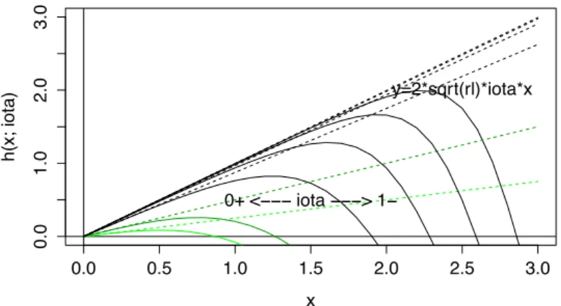
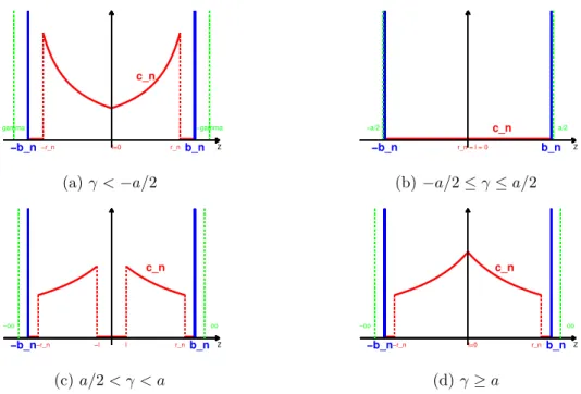
Under our framework, a candidate strategy Xb,c,Ÿ is indexed by two non-negative functions

b(s, t) and c(z, s, t). Let ZŸ = (X–≠ Xb,c,Ÿ_{)/Ÿ be the normalized deviation of X}b,c,Ÿ _{from the} benchmark position X–_{. We consider X}b,c,Ÿ _{of the form}

dXb,c,Ÿ t = 1 Ÿsgn(Z Ÿ_)c(|ZŸ t|, St, t)dÈX–Ít≠ ŸdLtŸ+ ŸdRŸt, X0+b,c,Ÿ = X0–, where LŸ _{and R}Ÿ _{are non-decreasing processes such that}

LŸ_t = ⁄ t 0 1{Zu=≠b(SuŸ ,u)}dL Ÿ u, RŸt = ⁄ t 0 1{ZuŸ=b(Su,u)}dR Ÿ u, |ZtŸ| Æ b(St, t). Intuitively, the regular control part Ÿ≠1_sgn(ZŸ)c(|ZŸ

t|, St, t)dÈX–Ítpushes Xb,c,Ÿ toward X–and is active when X–_{moves. The singular control part ≠ŸdL}Ÿ

t+ŸdRŸt keeps ZŸwithin the stochas-tic interval [≠b(St, t), b(St, t)], and is active only when ZŸ touches the boundary.

(17)

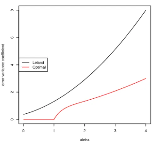
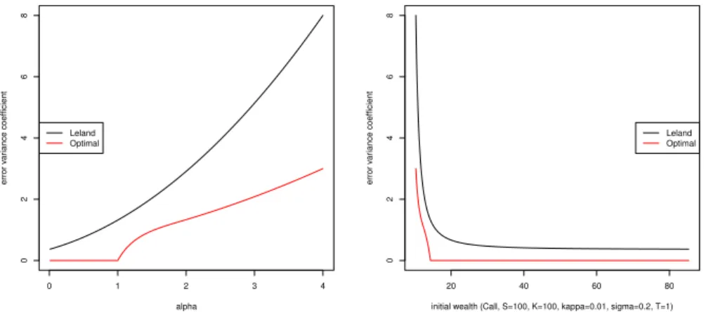
0 1 2 3 4 02468 alpha error v ar iance coefficient Leland Optimal

Figure 1 – Comparison between ÷L(–) and ÷†(–).

Denoting by b,c,Ÿ the wealth process associated with Xb,c,Ÿ and Eb,c,Ÿ the process of tracking error associated with the strategy Xb,c,Ÿ_{, we have}

Etb,c,Ÿ = –t ≠ b,c,Ÿt = Ÿ⁄ t 0 Z Ÿ udSu+ ⁄ t 0 Suc(|Z Ÿ u|, Su, u)dÈX–Íu+ Ÿ2 ⁄ t 0 Su[dL Ÿ u+ dRŸu] ≠ ⁄ t 0 1 –‡ 2_S2 u –udu. Our first main result in Chapter 2 is the following.

Main Result 2 (Limit distribution of normalized hedging errors). Under general local volatility

model for S and technical conditions for b and c, we have Ÿ≠1 3 E_·b,c,Ÿ≠ ⁄ _· 0 ” b,c_(S t, t)dt 4 æ W_Qb,c · ,

stably in law on C[0, T ] as Ÿ æ 0, where W is an independent Brownian motion, Qb,c_· =

⁄ _·

0 ÷

b,c_(S

u, u)dÈSÍu,

and ”b,c_{, ÷}b,c _{are explicitly determined by b and c.}

Fixing the conditional bias of hedging error ”b,c _{= ”, it is natural to minimize the conditional} variance Qb,c. Our second contribution in this chapter is to provide an explicit expression for the infimum

Q”,ú := essinf_{(b,c) s.t. ”}b,c_©” Qb,c,

among all candidate strategies, together with a sequence of strategies (bú_{, c}ú_{) attaining}

asymptot-ically the infimum Q”,ú_{. Comparing to the strategy of Leland, the hedging error is significantly}

reduced. Indeed, it is shown in [DK10] that, following the strategy of Leland,

Ÿ≠1( –_≠ –,Ÿ) æ WQL, QL= ÷L(–) ⁄ _· 0 | – uSu|2dÈSÍu, where ÷L(–) = 1 fi– 2₊ 2 fi–+ 1 ≠ 2 fi.

On the other hand, taking ” = 0, our optimal strategy (bú_{, c}ú_{) satisfies}

Ÿ≠1( –≠ bú,cú,Ÿ) æ WQ0,ú, Q0,ú = ÷†(–)

⁄ _·

0 |

–

uSu|2dÈSÍu, where ÷_† has closed-form expression and is much smaller than ÷L, see Fig.1.

(18)

Part II : Asymptotic optimal tracking

To illustrate the type of problems treated in this part, we consider a government having two means of influencing the foreign exchange rate of its own currency:

1. By choosing the domestic interest rate. A higher interest rate encourages the investors to buy the domestic currency, and as a consequence this currency becomes more valuable and the exchange rate increases.

2. At selected times the government can intervene in the foreign exchange market by buying or selling large amounts of foreign currency. Such intervention is applied only at discrete time and can change the exchange rate instantaneously.

A fluctuating exchange rate is not suitable for the domestic economy due to the uncertainty that it creates. On the other hand, the application of the two policies to stablize the exchange rate is also costly. The objective of the government is to keep the exchange rate close to a given central parity with minimal costs. See [MØ97, CZ00] for more details.

Similar tracking problems arise naturally in various situations such as the management of an index fund ([PS04, Kor99]), discretization of hedging strategies ([Fuk14, RT14, GL14a]), portfolio selection under transaction costs ([KMK15, ST13, PST15, AMKS15]), trading under market impact ([MMKS14, LMKW14, GW15a, GW15b, GW15c, BSV15]) or illiquidity cost ([RS10, NW11]).

These problems have two common components:

1. A target with stochastic evolution. Usually the target is a benchmark portfolio or index which fluctuates as function of market conditions.

2. A cost structure representing the tracking effort and deviation from the target. In general, greater tracking effort is needed to maintain smaller deviation from the target.

This leads us to formulate the tracking problem as follows.

2.1 Formulation of the tracking problem

We consider a target whose dynamics (X¶

t) is modeled by a continuous Itô semi-martingale defined on a filtered probability space ( , F, (Ft)tØ0,P) with values in Rd such that

dX_t¶= btdt+ ÔatdWt.

Here, (Wt) is a d-dimensional Brownian motion and (bt), (at) are predictable processes with values in Rdand the set S+

d of d ◊ d symmetric positive definite matrices respectively. An agent observes X¶

t and adjusts her position Âtin order to follow Xt¶. However, she has to pay certain intervention costs for position adjustments. The objective of the agent is to stay close to the target X¶

t while minimizing the tracking efforts. More precisely, let (Xt) be the deviation of the agent from the target (X¶

t), we have

Xt= ≠Xt¶+ Ât. (2.1)

Let H0(X) be a penalty functional for the deviation from the target and H(Â) the cost incurred

by the control process (Ât) up to horizon T . Denote by A the set of admissible strategies depending on the cost structure H0 and H. Then the problem of tracking can be formulated as

inf

(19)

Depending on the specific problem under consideration, the control process Â can be (the com-bination of) regular control, singular control or impulse control.

To fix idea, we consider in this introduction the case of combined regular and impulse control, which corresponds to the management of exchange rate mentioned above. In that case, a tracking strategy Â = (u, ·, ›) is given by a progressively measurable process u = (ut)tØ0 with values in

Rd and (·, ›) = {(·

j, ›j), j œ Nú}, with (·j) an increasing sequence of stopping times and (›j) a sequence of F·j-measurable random variables with values in R

d_{. The process (u}

t) represents the speed of the agent. The stopping time ·j represents the timing of jth jump toward the target and ›j the size of the jump. The tracking error obtained by following the strategy (u, ·, ›) is given by Xt= ≠Xt¶+ ⁄ t 0 usds+ ÿ j:0<·jÆt ›j.

At any time the agent is paying a cost for maintaining the speed ut and each jump ›j incurs a positive cost. We are interested in the following type of cost functional

J(u, ·, ›) = ⁄ T 0 (rtD(Xt) + l ¶ tQ(ut))dt + ÿ j:0<·jÆT (k¶ ·jF(›j) + h ¶ ·jP(›j)),

where (rt), (l¶t), (k¶t) and (h¶t) are random weight processes. The cost functions D, Q, F , P are deterministic functions defined for example by

D(x) = Èx, Dx_{Í, Q(u) = Èu,} Qu_{Í, F (›) =} d ÿ i=1 F_{i {›}i_”=0}, P(›) = d ÿ i=1 Pi|›i|,

with Fi, Pi œ R+ such that miniFi >0 and D, Q are d ◊ d positive definite matrices. Note that we have

D(Áx) = Á’D_D(x), Q(Áu) = Á’Q_Q(u), F (Á›) = Á’F_F(›), P (Á›) = Á’P_P(›), (2.3)

for any Á > 0 and

’D = 2, ’Q= 2, ’F = 0, ’P = 1.

2.2 Asymptotic framework

Our first contribution in this part is to introduce an asymptotic setting for the tracking prob-lem (2.1)-(2.2). In general, the probprob-lem rarely admits explicit solution. Under our asymptotic framework of small tracking costs, we are able to establish an asymptotic lower bound for (2.2), which is related to the time average control of Brownian motion.

Assume that there exist Á > 0 and —Q, —F, —P >0 such that

l¶_t = Á—Q_l

t, kt¶= Á—Fkt, h¶t = Á—Pht. (2.4) Then the asymptotic framework of small tracking costs consists in considering the sequence of optimization problems indexed by Á æ 0

inf (uÁ_,·Á_,›Á_)œAÁJ Á_(uÁ_{, ·}Á_{, ›}Á_), with JÁ(uÁ, ·Á, ›Á) = ⁄ T 0 (rtD(X Á t) + Á—QltQ(uÁt))dt + ÿ j:0<·Á jÆT (Á—F_k ·Á jF(› Á j) + Á—Ph·Á jP(› Á j)),

(20)

and X_tÁ= ≠X_t¶+ ⁄ t 0 u Á sds+ ÿ j:0<·Á jÆt ›Á_j.

The key observation is that under such setting, the tracking problem can be decomposed into a sequence of local problems. More precisely, let {tÁ

k = k”Á, k = 0, 1, · · · , KÁ} be a partition of the interval [0, T ] with ”Á_{æ 0 as Á æ 0. Then we can write}

JÁ(uÁ, ·Á, ›Á) = KÁ_≠1 ÿ k=0 j_tÁÁ k(t Á k+1≠ tÁk), with jÁ_t = 1 ”Á 1 ⁄ tÁ k+”Á tÁ k (rtD(XtÁ) + Á—QltQ(uÁt))dt + ÿ j:tÁ k<·jÁÆtÁk+”Á (Á—F_k ·Á jF(› Á j) + Á—Ph·Á jP(› Á j)) 2

As Á tends to zero, we approximately have

JÁ(uÁ, ·Á, ›Á) ƒ ⁄ T

0 j

Á tdt.

Now consider the following rescaling of XÁ over the horizon (t, t + ”Á]:

Â

X_sÁ,t= 1 Á—X

Á

t+Á–—_s, sœ (0, TÁ],

with TÁ _{= Á}≠–—_”Á_{, where – = 2 and — > 0 is to be determined (here – = 2 is related to the} scaling property of Brownian motion). On the one hand, we have

dXÂ_sÁ,t =ÂbÁ,t_s ds+ Ò Â aÁ,ts dWÊsÁ,t+uÂÁ,ts ds+ d( ÿ 0<_Â·_jÁ,tÆs Â ›_jÁ), (2.5) where Â bÁ,t_s = ≠Á(–≠1)—b_t_+Á–—_s, ÂaÁ,t_s = a_t_+Á–—_s, WÊ_sÁ,t= ≠ 1 Á—Wt+Á–—s, Â uÁ,t_s = Á(–≠1)—uÁ_t_+Á–—_s, ›ÂÁ_j = 1 Á—› Á j, ·ÂjÁ,t= 1 Á–—(· Á j ≠ t) ‚ 0.

On the other hand, using the homogeneity properties (2.3) of the cost functions, we obtain

j_tÁ_ƒ 1 TÁ 1 ⁄ TÁ 0 ! Á—’D_r tD(XÂsÁ,t) + Á—Q≠(–≠1)’Q—ltQ(uÂÁ,ts ) " ds + ÿ 0<_Â·_jÁ,tÆTÁ ! Á—F≠(–≠’F)—_k tF(›ÂÁj) + Á—P≠(–≠’P)—htP(›ÂÁj) "2 .

The second approximation can be justified by the continuity of cost coefficients rt, lt, ktand ht. If there exists — > 0 such that

—’D = —Q≠ (– ≠ 1)’Q— = —F ≠ (– ≠ ’F)— = —P ≠ (– ≠ ’P)—, or equivalently, — = —F ’D+ – ≠ ’F = —P ’D+ – ≠ ’P = —Q ’D+ (– ≠ 1)’Q , (2.6)

(21)

where – = 2, then we have j_tÁ ƒ Á—’D_IÁ t, with I_tÁ= 1 TÁ 1 ⁄ TÁ 0 ! rtD(XÂsÁ,t) + ltQ(uÂÁ,ts ))ds + ÿ 0<_Â·_jÁ,tÆTÁ (ktF(›ÂÁj) + htP(›ÂjÁ) "2 . (2.7) It follows that Á≠—’DJÁ_ƒ ⁄ T 0 I Á tdt. (2.8)

We are hence led to study IÁ

t as Á æ 0, which is closely related to the time-average control problem of Brownian motion.

2.3 Main results

Lower bounds

In Chapter 3, we study IÁ

t and establish an asymptotic lower bound for (2.8). By suitably choosing ”Á_{, we have ”}Á _{æ 0 and T}Á _{æ Œ as Á æ 0. Then we have}_Â_bÁ,t

s ƒ 0 and ÂaÁ,ts ƒ at for

s _{œ (0, T}Á]. Therefore, the dynamics of (2.5) is approximately a controlled Brownian motion

with fixed diffusion matrix at. Hence (2.5) together with (2.7) can be approximately bounded from below by the optimal cost of time-average control problem of a Brownian motion, that is

I_tÁ& I(at, rt, lt, kt, ht), (2.9) with the term on the right hand side being defined as

I(a, r, l, k, h) = inf

(u,·,›)lim supSæŒ

1 SE Ë ⁄ S 0 ! rD(Xs) + lQ(us)"ds+ ÿ 0Æ·jÆS ! kF(›j) + hP (›)"È, (2.10) where dXs= ÔadWs+ usds+ d 1 ÿ 0<·jÆs ›j 2 . (2.11) Consequently, we obtain Á≠—’DJÁ _ƒ ⁄ T 0 I Á tdt& ⁄ T 0 Itdt,

as Á æ 0. The main contribution in Chapter 3 is to formulate rigorously the above result as the following.

Main Result 3 (Lower bound). There exists — explicitly determined by (2.6) such that, for all

” >0 and any sequence of admissible strategies {ÂÁ_{œ A}Á_{, Á >}0}, we have lim Áæ0+P Ë ₁ Á—’DJ Á_(ÂÁ_{) Ø}⁄ T 0 Itdt≠ ” È = 1, (2.12)

where It= I(at, rt, kt, ht, lt) is essentially the optimal cost of time-average control of Brownian

motion (2.10)-(2.11) with parameters frozen at time t.

Various versions of Main Result 3 under different cost structures are also presented in Chapter 3, together with a comprehensive list of explicit examples for I.

A key step in the proof of Main Result 3 is to justify rigorously (2.9). More precisely, we show that

lim inf Áæ0 P[I

Á

(22)

where IÁ

t is given by (2.5)-(2.7) and It= I(at, rt, lt, kt, ht) is given by (2.10)-(2.11). Inspired by [KM93] and [KS99], we apply weak convergence method on the empirical occupational measures and express the lower bound Itas the solution of an infinite dimensional linear programming on a suitable space of measures. Such characterization is essentially equivalent to (2.10)-(2.11) if we formulate the controlled Brownian motion through a controlled martingale problem (see [KS01]).

Feedback strategies

Our goal in Chapter 4 is to build strategies attaining the lower bounds (2.12). Following classical approaches, we are interested in a class of feedback strategies which consists in keeping the deviation Xt inside a time-dependent domain. Consider for example the case of combined regular and impulse control. Let (Gt) be a moving open bounded domain associated with jump rule (›t) from ˆGt to Gt, and (ut) be a continuous function from ¯Gt to Rd. The sequence of feed-back strategies (XÁ_{, u}Á_{, ·}Á_{, ›}Á_{) corresponding to the triplet (u}

t, Gt, ›t) can be constructed in the following recursive way :

1. Let ·Á 0 = 0, X0Á= 0. 2. For t Ø ·Á j≠1, let XtÁ be defined by dX_tÁ= ≠dX_t¶+ uÁ_tdt, with uÁ_t = Á≠(–≠1)—ut(Á≠—XtÁ). 3. Set ·_jÁ= inf{t > ·_jÁ_≠1, 1 Á—X Á t œ G/ t}, ›jÁ= Á—›·Á j(Á ≠—_XÁ ·Á j≠), and X_·ÁÁ j = X Á ·Á j≠+ › Á j.

We now give the main result for combined regular and impulse control in Chapter 4. The cases involving singular control are also studied in same chapter.

Main Result 4 (Feedback strategies). Let {(XÁ_{, u}Á_{, ·}Á_{, ›}Á_{), Á > 0} be the feedback strategy}

determined by an admissible triplet (ut, Gt, ›t), then we have 1 Á—’DJ Á_(uÁ_{, ·}Á_{, ›}Á_{) æ} p ⁄ T 0 c(ut, Gt, ›t)dt,

where c(u, G, ›) can be explicitly determined via the stationary measures of Brownian motion in the domain G with drift u and jump rule › from the boundary.

For a wide range of examples, we show that there exists explicit triplet (uú

t, Gút, ›út) verifying

c(uú_t, Gú_t, ›_tú) = It. Hence, the associated feedback strategy {(XÁ,ú, uÁ,ú, ·Á,ú, ›Á,ú), Á > 0} satisfies 1 Á—’DJ Á_(uÁ,ú_{, ·}Á,ú_{, ›}Á,ú_{) æ} p ⁄ T 0 Itdt.

In other words, the asymptotic lower bound in Main Result 3 is tight.

2.4 Relation with other asymptotic studies

Our final contribution in Chapter 4 is to establish a link among different asymptotic analysis in the literature on various topics such as optimal discretization of hedging strategies, discretiza-tion error of stochastic integrals and impact of small market fricdiscretiza-tions.

(23)

Main Result 3 and 4 enable us to revisit the asymptotic lower bounds for the discretization of hedging strategies in [Fuk11a, GL14a]. In these papers, the lower bounds are deduced by using subtle inequalities. We show that theses bounds can be simply interpreted through the time average control problem of Brownian motion.

As a corollary of Main Result 4, we establish a weak convergence theorem for discretization errors of stochastic integrals with random stopping times. The limit law of the normalized discretization errors turns out to be a mixture of Gaussian distributions, with the conditional mean and variance being expressed as the first and second moments of the stationary measures of Brownian motion in a domain with jumps from the boundary. Our approach suggests that the results in [HM05, Fuk11c, Roo80, LR13] can be interpreted in a similar way.

The lower bound (2.12) appears also in the study of small market frictions under the framework of utility maximization. Indeed, we observe that utility maximization under small market frictions is heuristically equivalent to the tracking problem with the target being the optimal strategy under frictionless market. Consider, for example, the optimization of terminal wealth given by

u(w₀) = sup

Ï E[U(w Ï T)],

where w0 is the initial wealth and wTÏ the terminal wealth following the trading strategy Ï. In a market with proportional transaction costs, the portfolio dynamics is given by

wÁ_t = w₀+ ⁄ t 0 Ï Á udSu≠ ⁄ t 0 ÁhudÎÏ Á_Î u,

where Stis the risky asset price, Áht is a random weight process representing transaction costs, and ÏÁ

t is a trading strategy with finite variation. Assume that Ïút is the optimal trading strategy in the frictionless market (Á = 0), and denote the equivalent martingale measure by Q and the indirect risk-tolerance process by Rt. When Á is small, we can expect that ÏÁt is close to Ïút. Then up to first order quantities, we have (see also [KMK15, KL13, Rog04])

E[U(wÁ T)] ≠ u(w0) ƒ ≠uÕ(w0)EQ Ë Á ⁄ T 0 htdÎÏ Á_Î t+ ⁄ T 0 aS_t 2Rt(Ï Á t≠ Ïút)2dt È , where aS

t is the quadratic variation of the risky asset St. Hence the optimization of terminal wealth under small proportional costs can be reduced to a tracking problem with stochastic target Ïú

t and deviation penalty

rtD(x) :=

aS_t

2Rt

x2.

Denoting the value function under transaction costs by uÁ_{, and defining the certainty equivalent} wealth loss Á _by uÁ=: u(w₀_≠ Á), then we have 1 Á—’D Á_{ƒ E}Q_[⁄ T 0 Itdt].

Similar correspondences can also be established for the cases with different cost structures ([AMKS15, MMKS14]), the indifference pricing of option ([WW97, WW99, KMK13]), the max-imization of long term growth rate ([AW95, APW97, GW15a, GW15b, GW15c, LMKW14]), and optimization of consumption ([ST13, PST15]).

(24)

Part III : Portfolio selection with capital gains taxes

In contrast to transaction costs, the problem of portfolio selection under capital gains taxes received relatively limited attention. Capital gain taxes differ from transaction costs in the following aspects:

1. Investors pay taxes for capital gains but receive tax rebates for capital losses.

2. The amount of capital gains or losses taxed depends on the purchase price of stock holdings, known as the tax basis, which incurs strong path-dependency.

As a consequence, much of the existing literature on capital gain taxes has been restricted to discrete-time models with small number of time steps, see [Con83, Con84, DK96, DU05, GH06]. Using the average purchase price of stocks as an approximation for tax basis, [DSZ01, DSZ03] develop a binomial tree model that is able to effectively work with multi-step investment and consumption decisions. The advantage of the approximation is that the path dependency of the problem is considerably reduced, as the dynamics of the tax basis becomes Markovian. [GKT06] further extend the model to the multiple stocks case. In [BST10], the authors formu-late a continuous-time version of the model introduced by [DSZ01].

In this part, we are interested in the joint impact of capital gains taxes with other market fea-tures such as regime-switching and transaction costs. Our work is mainly based on extensions of the models of [BST10, BST07]. We point out that the goal of this part is to provide a deep un-derstanding of the optimal strategy and related probabilistic interpretation, although the main results remain to be rigorously proved.

3.1 Preliminary : the model of [BST10]

Let us describe the model of [BST10] in more details. Consider a financial market with two assets that the investor can trade without any transaction costs. The first asset is a bond with pre-tax interest rate r. The second asset is a risky stock whose price (St) evolves according to the Black-Scholes model:

dSt= St(µdt + ‡dWt).

The investor is subject to capital gain taxes. The tax basis (Bt) used to evaluate capital gains is defined as the weighted average of past purchase prices. The amount of tax to be paid for each sale of risky asset is given by

–(St≠ Bt),

where – œ [0, 1). When StØ Bt, i.e. the current price of the risky asset is greater than the tax basis, the investor realizes a capital gain by selling the risky asset. When St < Bt, the sale of the risky asset corresponds to the realization of a capital loss.

Let Xt, Yt, and Kt be the amount invested in the bond, the current dollar value of, and the cumulated purchase price of stock holdings, respectively. We introduce two càdlàg, non-negative, and non-decreasing Ft-adapted processes Ltand Mtwith L0≠= M0≠ = 0, where dLtrepresents the dollar amount transferred from the bank to the stock account at time t (corresponding to a purchase of stock), while dMt represents the proportion of shares transferred from the stock account to the bank at time t (corresponding to a sale of stock). We assume the no-short-sales constraint such that dMt Æ 1. Note that the cumulated purchase price of stock holding Kt is related to the tax basis Bt by

Kt= Bt

Yt

St

(25)

Hence, when one sells stock at time t, the cumulated purchase price Kt declines by the same proportion dMt as the dollar value of stock holdings does, and the realized capital gain is (Yt≠≠ Kt≠)dMt. Then, the evolution processes of Xt, Yt, and Kt are

dXt = [(1 ≠ –)rXt≠ Ct] dt ≠ dLt+ [Yt≠≠ – (Yt≠≠ Kt≠)] dMt,

dYt = Yt(µdt + ‡dWt) + dLt≠ Yt≠dMt,

dKt = dLt≠ Kt≠dMt, where (Ct) is the consumption stream. The investor aims to find

Ï(x, y, k) := sup (Ct,Lt,Mt) EË ⁄ Œ 0 e ≠—t_U_(C t, “)dt--X0 = x, Y0 = y, K0 = k È , (3.1)

where — > 0 is a constant discount factor and U(·, “) is a power utility function with parameter “. Since the value function (3.1) admits no closed-form solution, [BST10] provide instead analytical upper and lower bounds. First, if there is no capital gains taxes (– = 0), then the above problem reduces to the classical tax-free Merton problem. Denote the value function of the Merton problem by ¯Ï and the optimal consumption-investment strategy by (¯c, ¯›). Second, consider the following tax-free model with parameters

µ–= (1 ≠ –)µ, ‡–= (1 ≠ –)‡, r– = (1 ≠ –)r. (3.2)

This is the so called tax-deflated model. Denote the value function of the corresponding Merton problem by ¯Ï– and the optimal consumption-investment strategy by (¯c–, ¯›–). Then it is shown in [BST10, Propostion 4.1, 4.2] that,

¯Ï–(z) Æ Ï(x, y, k) Æ ¯Ï(z), (3.3)

where z is the liquidation wealth z = x + y ≠ –(y ≠ k).

While the upper bound is natural in that the investor cannot take advantage of tax rebates to do better than in a tax-free market, [BST10] provide an insight for the lower bound. More precisely, define the portfolio value after liquidation Ztby

Zt= Xt+ Yt≠ –(Yt≠ Kt). Then we have dZt= dXt+ (1 ≠ –)dYt+ –dKt = [(1 ≠ –)rZt≠ Ct]dt + (1 ≠ –)Yt(µdt + ‡dWt≠ (1 ≠ –)rdt) ≠ (1 ≠ –)–rKtdt. Taking ›t= Yt Zt , bt= Kt Yt , ct= Ct Zt , (3.4) we obtain dZt= Zt#(r–≠ ct)dt + ›t(µ–dt+ ‡–dWt≠ r–dt) + –r–›t(1 ≠ bt)dt$. (3.5) The process btØ 0 is called the relative tax basis. Note that bt>1 corresponds to capital losses while bt<1 corresponds to capital gains. By constructing a sequence of strategies which keeps asymptotically bt© 1, [BST10] show that Zt can be approximated by

dZt= Zt#(r–≠ ct)dt + ›t(µ–dt+ ‡–dWt≠ r–dt)$,

which is exactly the wealth process under the tax-deflated model (3.2). The lower bound follows from the possibility to replicate (asymptotically) any consumption stream which is admissible for the tax-deflated model under the model of [BST10].

(26)

3.2 Expansion around tax-deflated model

Our first contribution in Chapter 5 is to improve the bounds in (3.3) by providing a first order correction in terms of a time-average control problem. The sub-optimal stratey b1 © 1 proposed

by [BST10] consist in realizing both capital losses and gains immediately. We observe that keep-ing bt© 1 is apparently not the optimal choice. Indeed, as long as 1 ≠ btØ 0, the last term in (3.5) is in the favor of the investor. Therefore, it is better for the investor to defer capital gains and keep bt Æ 1. Meanwhile, such deferral will drive the portfolio away from the benchmark ¯›– under the tax-deflated model. Hence the optimal strategy should be a delicate balancing between capital gains deferral and the utility loss due to deviation from the benchmark optimal strategy ¯›– under the tax-deflated model.

The main idea is to consider the asymptotic setting where the interest rate or tax rate are small. Then the extra benefit from tax deferral –r–›t(1 ≠ bt) is small and ›t≠ ¯›– should also be small. Using heuristic Taylor expansion as in [Rog04], we obtain

EË ⁄ Œ 0 e ≠—t_U_(C t, “)dt È ƒ ¯Ï–(z) + (1 ≠ “)U(¯c–z, “) ⁄ _Œ 0 e ≠¯c–tEQ–Ë ⁄ t 0 (–r–›s(1 ≠ bs) ≠ “‡_–2 2 (›s≠ ¯›–)2)ds È dt.

where Q– is a suitable change of probability.

In order to obtain extra welfare by tax-deferral, the investor needs essentially to maximize EQ–Ë ⁄ t 0 (–r–›s(1 ≠ bs) ≠ “‡2_– 2 (›s≠ ¯›–)2)ds È , (3.6)

where the first term represents the benefit of tax-deferral and the second the equivalent wealth loss due to deviation from the benchmark strategy ¯›–. Applying Itô formula to (3.4), it is not difficult to deduce the dynamics of ›t and bt :

dbtƒ ≠‡btdWt+1 ≠ b_{¯› dD}t t+ dRt,

d(1 ≠ –)›tƒ ‡ ¯›(1 ≠ ¯›)dWt+ dDt≠ dUt,

(3.7) where Dt, Ut and Rt are processes with finite variation determined by Lt and Mt.

An interesting property of the coupled system (3.7) is that

›t≠ ¯›–= O(”2) … 1 ≠ bt= O(”). In other words, 1 ≠ bt and ›t≠ ¯›– have different time scales. Defining

pt= 1 ≠ bt ” , qt= ›t≠ ¯›– ”2 , where ”= (AÁ)2/3, Á= Û 2–r–¯›– “‡2 , A= 4 [3¯›(¯›≠ 1)]2,

and applying similar arguments as in the tracking problem, we are led to consider the following time-average control problem in which the fast variable qt disappears:

I” = sup (lt)lim infTæŒ 1 TE Ë ⁄ T 0 (pt≠ 1 3A2lt2)dt È , (3.8)

(27)

and the dynamics of ptbecomes

dpt= ‡(1 ≠ ”pt)dWt≠

‡2

3Alt

ptdt+ dRt, (3.9)

where ltis an adapted positive process and Rta non-decreasing process representing the reflection of pt at p = 0. Our first contribution in Chapter 5 is the following result, which is only heuristically proved.

Main Result 5. Taking z = x + y ≠ –(y ≠ k) and defining the value of tax deferral w by

Ï(x, y, k) = ¯Ï–(zew), then we have w= “ ¯c– ‡2 2 I”A2/3Á8/3+ o(Á8/3),

where I” _{is given by the optimal cost of the time-average control problem (3.8)-(3.9).}

Compare to the case of utility maximization with market frictions, we have identified a new local probabilistic model (3.8)-(3.9) in the first order expansion of the value function.

3.3 Capital gains taxes with recursive utility and regime-switching

Our second contribution in Chapter 5 is to study the impact of capital gains taxes in a regime-switching market for an investor with recursive utility of Epstein-Zin type. We not only provide asymptotic analysis based on the intuition developed in the previous section, but also perform extensive numerical study to validate our asymptotic analysis.

Let Ïi be the value function under regime i œ I. As before, we introduce the tax-deflated regime-switching model for which the market parameters r–,i, µ–,i and ‡–,i are given by

r–,i = (1 ≠ –)ri, µ–,i = (1 ≠ –)µi, ‡–,i = (1 ≠ –)‡i, ’i œ I.

We denote the value function of tax-free problem under regime i by ¯Ï–,iand the optimal strategy by (¯c–,i, ¯›–,i). The main result of Chapter 5 is the following heuristic expansion of value function.

Main Result 6. Defining the value of deferral wi under regime i by

Ïi(x, y, k) = ¯Ï–,i(zewi), then we have wi = “ ¯c–,i ‡2_i 2 miA2/3i Á 8/3 i + o(Á 8/3 i ),

where {mi, iœ I} are explicitly determined in term of {I”i, iœ I} via a linear system.

The key step to obtain the above expansion is first suggested in [CD13], where the authors use the following “fast variables”

pi= 1 ≠ k/y

”i

, qi =

y/z≠ ¯›–,i

”_i2 ,

and postulate in the associated HJB equation that

wi= “Á2i 1 ”i ‡_i2 2 1 ¯c–,i mi+ ”3igi”(pi) + ”5ivi”(pi, qi) 2 .

(28)

This asymptotic setting is now fully supported by our probabilistic analysis in Section 3.2. The asymptotic expansion allows us to perform fruitful economic analysis of the impact of cap-ital gains taxes. In particular, we obtain the impact of capcap-ital gains taxes in function of the elasticity of inter-temporal substitution (EIS) and regime transition intensities, together with explicit trading boundaries. Moreover, these asymptotic analysis are all validated by a direct numerical computation of the associated HJB equation based on penalty method.

3.4 Joint impact of capital gains taxes and transaction costs

Our goal in Chapter 6 is to derive a system of corrector equations for the value function of port-folio selection problem under proportional transaction costs and capital gains taxes, extending both [ST13] and [CD13]. Models with both transaction costs and capital gains taxes have also been studied in [CP99, BCP05, Lel99] but under quite different settings.

For simplicity, we use the model of [BST07] and keep the same notation as in Section 3.1. Given any strategy (Ct, Lt, Mt), the dynamics of Yt and Ktremain the same and we have

dXt= ((1 ≠ –)rXt≠ Ct)dt ≠ (1 + ⁄B)dLt+ (1 ≠ ⁄S)[(1 ≠ –)Yt≠+ –Kt≠]dMt,

where ⁄B, ⁄S œ [0, 1) represent the buy/sell costs and – œ [0, 1) is the tax rate. In the asymptotic setting of small transaction costs and interest rate, we replace the transaction cost coefficients

⁄B, ⁄S and the interest rate r by

⁄”_B= ⁄B”6, ⁄”S = ⁄S”6, r” = r”3, ” >0.

and denote the corresponding value function by Ï”_{(x, y, k). The associated tax-deflated model} is defined by

µ– = (1 ≠ –)µ, ‡– = (1 ≠ –)‡, r–” = (1 ≠ –)r”.

Denote the value function of Merton problem under the tax-deflated model (without transaction costs and taxes) by ¯Ï”

–(z), and the corresponding optimal consumption-investment strategy by ( ¯C”

–(z), ¯y”–(z)). The main contribution of Chapter 6 is the formal derivation of the following corrector equations.

Main Result 7. Taking z = x + y ≠ –(y ≠ k), we have

Ï”(x, y, k) = ¯Ï”_–(z) + u”_–(z)”4+ o(”4), where u”

– is given by

≠1₂‡_–2(¯y_–”(z))2ˆ2_zzu”_–(z) ≠ [(µ–≠ r–”)¯y–”(z) + r–”z≠ ¯C–”(z)]ˆzu”–(z) + —u”–(z) ≠ a(z) = 0.

The constant a(z) (depending on z) is determined by

minÓ≠1₂‡2(1 ≠ ”p)2ˆ2_ppG_–”(z, p) ≠!–r–ˆz¯Ï”–(z)¯y”–(z)p ≠ b(z, p) "_{+ a(z),} G”_–(z, p) + (⁄S+ ⁄B)ˆz¯Ï”–(z)¯y–”(z) ≠ G”–(z, 0) Ô = 0, and minÓ1 2‡2(¯y–”(z))2[1 ≠ (1 ≠ –)ˆz¯y–”(z)]2ˆqq2 w”–(z, p, q) + 1 2‡2–(≠ˆzz2 ¯Ï”–(z))q2≠ b(z, p), p ¯y” –(z) ˆpG”–(z, p) + ⁄Bˆz¯Ï”–(z) ≠ ˆqw”–(z, p, q), ≠⁄Sˆz¯Ï”–(z) ≠ ˆqw”–(z, p, q) Ô = 0.

(29)

In particular, we recover the corrector equations in [ST13, Definition 3.1] if – = 0, and [CD13, Equation (A.13)] if ⁄B= ⁄S = 0.

In [ST13, Remark 3.3], the equation for w”

–(q) is represented by the time-average control of Brownian motion with proportional costs. We find that the equation for G”

–(p) is also closely related to a time-average control problem like (3.8)-(3.9) and a(z) can be interpreted as the corresponding optimal cost I”_.

(30)

(31)