HAL Id: hal-00731864
https://hal.sorbonne-universite.fr/hal-00731864
Submitted on 13 Sep 2012
HAL is a multi-disciplinary open access
archive for the deposit and dissemination of
sci-entific research documents, whether they are
pub-lished or not. The documents may come from
teaching and research institutions in France or
abroad, or from public or private research centers.
L’archive ouverte pluridisciplinaire HAL, est
destinée au dépôt et à la diffusion de documents
scientifiques de niveau recherche, publiés ou non,
émanant des établissements d’enseignement et de
recherche français ou étrangers, des laboratoires
publics ou privés.
Facial Action Recognition Combining Heterogeneous
Features via Multi-Kernel Learning
Thibaud Sénéchal, Vincent Rapp, Hanan Salam, Renaud Seguier, Kevin
Bailly, Lionel Prevost
To cite this version:
Thibaud Sénéchal, Vincent Rapp, Hanan Salam, Renaud Seguier, Kevin Bailly, et al.. Facial Action
Recognition Combining Heterogeneous Features via Multi-Kernel Learning. IEEE Transactions on
Systems, Man, and Cybernetics, Part B: Cybernetics, Institute of Electrical and Electronics Engineers,
2012, 42 (4), pp.993-1005. �10.1109/TSMCB.2012.2193567�. �hal-00731864�
JOURNAL OF LATEX CLASS FILES, VOL. 6, NO. 1, JANUARY 2007 1
Facial Action Recognition Combining
Heterogeneous Features via Multi-Kernel Learning
Thibaud Senechal, Member, IEEE, Vincent Rapp, Member, IEEE,
Hanan Salam, Renaud Seguier, Kevin Bailly and Lionel Prevost.
Abstract—This paper presents our response to the first interna-tional challenge on Facial Emotion Recognition and Analysis. We propose to combine different types of features to automatically detect Action Units in facial images. We use one multi-kernel SVM for each Action Unit we want to detect. The first kernel matrix is computed using Local Gabor Binary Pattern histograms and a histogram intersection kernel. The second kernel matrix is computed from AAM coefficients and an RBF kernel. During the training step, we combine these two types of features using the recently proposed SimpleMKL algorithm. SVM outputs are then averaged to exploit temporal information in the sequence. To eval-uate our system, we perform deep experimentations on several key issues: influence of features and kernel function in histogram-based SVM approaches, influence of spatially-independent in-formation versus geometric local appearance inin-formation and benefits of combining both, sensitivity to training data and interest of temporal context adaptation. We also compare our results to those of the other participants and try to explain why our method had the best performance during the FERA challenge.
Index Terms—Facial Action Unit, LGBP, AAM, Multi-kernel learning, FERA challenge
I. INTRODUCTION
A current challenge in designing computerized environ-ments is to place the human user at the core of the system. It is argued that to truly achieve effective Human-Computer Intelligent Interaction (HCII), there is a need for the computer to be able to interact naturally with the user, similar to the way human-human interaction takes place. Traditional computer interfaces ignore user affective states, resulting in a large loss of valuable information for the interaction process. To recognize affective state, human-centered interfaces should in-terpret non verbal behavior like voice, body gestures and facial movements. Among all these topics, facial expression is the most natural way for human beings to communicate emotions and interact with other people. This can explain why Facial Expression Recognition and Analysis (FERA) is an active topic in the fields of pattern recognition, computer vision and human-computer interface. Psychological research has shown that facial expressions and head movements are social signals helping information transfer between humans. Experiments in [1] show the superiority of these clues over voice tone or spoken word (representing respectively 55%, 38% and 7% of
T. Senechal, V. Rapp and K. Bailly are with UPMC Univ. Paris 06, CNRS UMR 7222, ISIR, F-75005, Paris, France.
L. Prevost is with Univ. of French West Indies & Guiana, EA 4540, LAMIA, Guadeloupe, France
H.Salam and R.Seguier are with Supelec, CNRS UMR 6164, IETR, 35511, Cesson-Sevigne, Frances
the total meaning). They are widely cited and criticized as extremely weakly founded. Nevertheless, later studies [2], [3] show that rapid facial movements convey information about people affective states, moods and personality. They complete, reinforce the verbal message and are sometimes used as the sole channel for communicating messages [4]. Automated analysis of such signals should increase the effectiveness of Animated Conversational Agents (ACA) and assisting robots [5]. It should also impact researches in social psychology and psychopathology. Finally, by capturing the subtle movement of human facial expression, it could increase the rendering quality of ACA and bridge the ”uncanny valley”.
The original emotional taxonomy was defined in the early 70s by Ekman [6] as a set of six basic universal facial emo-tions (anger, disgust, fear, happiness, sadness, and surprise). These basic emotions can be combined to form complex emotions. While this basic emotions theory is discrete, the dimensional approach [7] is continuous. Emotion can vary continuously in a two (or more) dimensional space formed (at least) by the dimensions valence (positive/negative) and arousal (calm/excited). Another standard way is to describe the set of muscle movements that produce each facial expression. These movements are called facial Action Units (AUs) and the corresponding code is the so-called Facial Action Coding System (FACS) [8]. These AUs are combined in order to create the rules responsible for the formation of facial expressions as proposed in [9]. Some scientific issues concerning expression are: spontaneous versus posed expression recognition, speech versus non-speech expression recognition, temporal expression segmentation or modeling the dynamic of expression.
This paper mainly focuses on AU detection (though emotion recognition is also discussed) on the GEMEP-FERA database (described in the section I-A). It is interesting to compare this database with standard databases like Cohn-Kanade database or MMI database. The main difference with Cohn-Kanade database is that emotion displayed by actors are much more spontaneous and natural. Sequences do not begin on the neutral state to end on the apex expressive state. Contrary to both (Cohn-Kanade and MMI) databases, people are less posed (in term of face pose) and emotion is more natural and sometime more subtle and less caricatured. Moreover, the GEMEP-FERA database includes speech therefore a greater variability in the appearances of the lower face AUs. This is clearly one step towards real word conditions but expression recognizer must be able to deal with this increasing complexity. Simple emotion recognizer based on a single set of geometric or appearance features may fail here. This is why we propose
to combine heterogeneous features in an original framework (described in section I-B) to take advantages of both geometric and appearance features. The analysis of challenge results (section VI-E) shows we are right.
A. Challenge context and data
Many systems have been proposed in the literature, but they all lack a common evaluation protocol. This contrasts with more established problems in human behavior analysis from video such as face detection and face recognition (like FRGC [10] or FERET [11]). The Facial Expression and Analysis challenge (FERA), organized in conjunction with the IEEE International conference on Face and Gesture Recognition 2011, allows a fair comparison between systems vying for the title of ”state of the art”. To do so, it uses a partition of the GEMEP corpus [12], developed by the Geneva Emotion Research Group (GERG) at the University of Geneva led by Klaus Scherer. The challenge is divided in two sub-challenges reflecting the main streams in facial expression analysis: emotion detection and Action Unit detection. The AU detection sub-challenge calls for researchers to attain the highest possible F1-measure for 12 frequently occurring AU. The GEMEP corpus consists of over 7000 audiovisual emotion portrayals, representing 18 emotions portrayed by 10 actors. A subset of the GEMEP corpus was annotated in terms of facial expression using the FACS and used in the AU detection sub-challenge.
B. Overview of the proposed method
Most of the existing approaches to detect AUs fall into three categories depending on the type of feature used (see Section II). The first, and oldest, category includes geometric feature-based methods, the second includes appearance feature-feature-based methods while the last considers all the methods that use both geometric and appearance features. As geometric and appearance feature-based methods have their own advantages and drawbacks, we decide, as participant, to combine both. We use classical image coding schemes: Local Gabor Binary Pat-tern (LGBP) histograms with shape and texture parameters of an Active Appearance Model (AAM). LGBPs, introduced by Zhang et al. [13] for face recognition, exploit multi-resolution and multi-orientation links between pixels and are very robust to illumination variations and misalignment. Moreover, the use of histograms results in the loss of spatial information which really depends on identity. One of the drawbacks would be the inability to capture some subtle movements useful for Action Unit detection. To deal with it, we decide to look for another set of features that does not lack this information. So, we choose to use the Active Appearance Model (AAM) introduced by Cootes et al. [14]. An AAM is a statistical model of the shape and grey-level appearance of the face which can generalize to almost any valid example. AAMs can provide important spatial information of key facial landmarks but are dependent of an accurate matching of the model to the face images.
To perform AU detection, we select Support Vector Ma-chines (SVM) for their ability to find an optimal separat-ing hyper-plane between the positive and negative samples
in binary classification problems. As both features (LGBP histograms and AAM coefficients) are very different, we do not concatenate them in a single vector. Instead of using one single kernel function, we decide to use two different kernels, one adapted to LGBP histograms and the other to AAM coefficients. We combine these kernels in a multi-kernel SVM framework [15]. Finally, to deal with temporal aspects of action unit display, we post-process the classification outputs using a filtering and a thresholding technique.
In addition to detailing the steps of the AUs detector con-ception for the FERA challenge, this article tries to emphasize with rigorous experiments, the benefit of combining features and the AU labels compatibility between databases.
The paper is organized as follows. Section II provides an overview of the related research. Section III describes image coding and details LGBP histogram and AAM coef-ficient calculation. Section IV explains classification process to detect AUs in facial images and post-processing temporal analysis. Section V details experiments to validate the choice of LGBP histograms and the histogram intersection kernel. Section VI reports AUs detection results on the GEMEP-FERA test dataset. Section VII reports emotion recognition results. Finally section VIII concludes the paper.
II. STATE OF THE ART
The general flowchart of automated facial expression anal-ysis in video sequences consists of several steps. The first step concerns face registration (including face detection and landmarks localization). The second one is image coding. The third one classifies frames as positive (a single AU, an AU combination or an emotion has occurred) or negative. Finally, the last step is the temporal analysis.
The objective of the face registration step is to normalize the image. Some simple normalization methods remove in-plane rotation and scaling according to the eyes localization, while other approaches try to remove small 3D rigid head motion using an affine transformation or a piece-wise affine warp [16]. Whatever the methods are, image registration relies on preliminary face detection and facial landmarks localization. Face detection is usually based on the public OpenCV face detector designed by Viola and Jones [17] that applies an attentional cascade of boosted classifiers on image patches to classify them as face or non-face. Recent improvements of this algorithm are presented in [18]. Once the face is detected, there are two main streams for facial landmark localization. The first is based on a classification framework. Detections can be performed using a GentleBoost classifier [19] or a MK-SVM [20] to deal with multi-scale features. Simple prior information on facial landmark relative positions is used to avoid some outliers. The second approach directly aligns the face by using some kind of deformable model. For example, Koatsia and Pitas [21] exploit the Candide grid, Asthana et al. [22] compare different AAM fitting algorithms and Saragih et al. [23] use Constrained Local Models. Some approaches are based on 3D face models. Wen and Huang [24] use a 3D face tracker called Piecewise Bezier Volume Deformation Tracker (PBVD) and Cohn et al. [25] apply a cylindrical head model to
JOURNAL OF LATEX CLASS FILES, VOL. 6, NO. 1, JANUARY 2007 3
analyze brow AUs and head movements. The main drawback of this approach is the necessity of labeling manually some landmark points in the first sequence frame before warping the model to fit these points.
Most of the existing approaches to detect either AUs or emotions fall into three categories: those that use geometric features, those that use appearance features and those that combine both geometric and appearance features. For an extensive overview of facial expression recognition, we invite the reader to consult [26]
Geometric-based methods try to extract the shape of facial components (eyes, mouth, nose, etc.) and the location of facial salient points. Depending on the previous alignment step, these can either be a set of fiducial points or a connected face mesh. Previous works of Pantic and colleagues were based on the first strategy. Typically, in [27], they track 20 facial feature points along sequences. These points of interest are detected automatically in the first frame and then, tracked by using a particle filtering scheme that uses factorized likelihoods and a combination of a rigid and a morphological model to track the facial points. The AUs displayed are finally recognized by SVMs trained on a subset of most informative spatio-temporal features.
On the other hand, Cohen et al. [28] use a PBVD tracker to follow the movement of 12 facial points in sequences expressed in term of ”Motion units”. They use a Bayesian classifier to deal with still images and Hidden Markov Models (HMM) to recognize emotions in a video sequence. They also propose a multi level HMM to combine temporal information and automatically segment an arbitrary long video sequence. Using the same tracking method, Sebe et al. [29] tested and compared a wide range of classifiers from the machine learning community including Bayesian networks, decision trees, SVM, kNN, etc.
Appearance-based methods extract features that try to repre-sent the facial texture including wrinkles, bulges and furrows. An important part of these methods relies on extracting Gabor Wavelets features especially to detect AU. These features have been widely used due to their biological relevance, their ability to encode edge and texture and their invariance to illumination. Bartlett et al. [30] use these features with a GentleBoost-SVM classifier, Bazzo and Lamar [31] with a neural network and Tong et al. [32] with a Dynamic Bayesian Network to exploit AU relationships and AU dynamics. Other features successfully used in AU detection are the Haar-like features with an adaboost classifier proposed by Whitehill and Omlin [33] or the Independent Components combined with SVMs by Chuang and Shih [34]. For the emotion recognition task, Moore et al. [35] combine Local Gabor Binary Pattern (LGBP) histograms with SVM and Fasel et al. [36] combine gray-level intensity with a neural network classifier. The challenge organizers provide a baseline method [37] where LBP are used to encode images, Principal Component Analysis to reduce features vector dimension and SVM classifier to provide either AU or emotion scores, depending on the task.
Some appearance-based methods try to extract temporal pattern inside sequences. A typical example is the optical flow extraction [38]. Valstar et al. [39] encoded face motion into
Motion History Images . Recently, Koelstra et al. [40] use dynamic Texture [41]. They extract motion representation and derive motion orientation histogram descriptors in both the spatial and temporal domain. Per AU, a combination of dis-criminative, frame-based GentleBoost ensemble learners and dynamic, generative HMM detects the presence of the AU and its temporal segment. Zhao and Pietikinen [42] apply volume Local Binary Patterns which are the temporal equivalent of LBP. In [19], Bartlett and colleagues Computer Expression recognition Toolbox (CERT) is extended to include temporal information. They show that frame-by-frame classifier accu-racy can be improved by checking temporal coherence along the sequence.
Finally, some studies exploit both geometric and appearance features. For example, Tian et al. [43] or Zhang and Ji [44] use facial points or component shapes with features like crow-feet winkles and nasal-labial furrows. Chew et al. [45] use a CLM to track the face and features and encode appearance using LBP. SVM are used to classify AUs. In [46], point displacements are used in a rule-based approach to detect a subset of AU while the others are detected using Gabor filters and SVM classifiers.
III. FEATURES
A. LGPB histograms
In this section, we describe how we compute Local Gabor Binary Patterns histograms from facial images (Fig. 1). To pre-process data, we automatically detect eyes using our own feature localizer [20]. Eyes localization is used to remove variations in scale, position and in-plane rotation. We obtain facial images with the same size pixels and eye centers remaining at the same coordinates.
1) Gabor magnitude pictures: The Gabor magnitude pic-tures are obtained by convolving facial images with Gabor filters : Gk(z) = k2 σ2e (−k2 2σ2z 2) (eikz− e−σ22 ) (1)
Where k = kveiφu is the characteristic wave vector. We use
three spatial frequencies kv = (π2,π4,π8) and six orientations
φu= (kπ6 , k ∈ {0 . . . 5}) for a total of 18 Gabor filters. As the
phase is very sensitive, only the magnitude is generally kept. It results in 18 Gabor magnitude pictures.
2) Local Binary Pattern (LBP): The LBP operator was first introduced by [47]. It codes each pixel of an image by thresholding its 3 × 3 neighborhood by its value and considering the result as a binary number. The LBP of a pixel p (value fp) with a neighborhood {fk, k = 0...7} is defined
as: LBP (pc) = 7 X k=0 δ(fk− fp)2k (2) where δ(x) = ( 1 if x ≥ 0 0 if x < 0 (3)
Face image Cropped and resized image Gabor magnitude pictures LGBP maps LGBP histograms
Fig. 1. Local Gabor Binary Pattern histograms computation.
3) Local Gabor Binary Pattern (LGBP): We apply the LBP operator on the 18 Gabor magnitude pictures resulting in 18 LGBP-maps per facial image. This combination of the Local Binary Pattern operator with Gabor wavelets exploits multi-resolution and multi-orientation links between pixels. This has been proven to be very robust to illumination changes and misalignments [13].
4) Histogram sequences: Each area of the face contains different useful information for AU detection. Thus, we choose to divide the face into several areas and compute one histogram per area. Such a process is generally applied in histogram-based methods for object classification. We divide each facial image into n × n non-overlapping regions in order to keep a spatial information. The optimal value of n will be discuss in section V-A. h(k) =X p I(k ≤ fp< k + 1), k = 0 · · · 255 (4) I(A) = ( 1 if A is true 0 if A is false (5) For each face i, we get one vector Hi by concatenating all
the histograms. Hi is the concatenation of 18 × n2histograms
computed on each region, orientation and spatial frequency resulting in 256 × 18 × n2 features per facial image.
5) Histogram reduction method: Ojala et al.[47] showed that a small subset of the patterns accounted for the majority of the texture of images. They only keep the uniform patterns, containing at most two bitwise transitions from 0 to 1 for a circular binary string.
To reduce the number of bins per histogram, we choose a slightly different approach. As we want the contribution of all patterns, we decide to group the occurrence of different patterns into the same bin. First, we only keep patterns be-longing to a subgroup of the uniform patterns: the 26 uniform patterns that have a pair number of ”1”. This subgroup has been chosen because all the uniform patterns are close to one bit to at least one pattern of this sub-group and the minimum distance between two patterns of this subgroup is 2. Then, all patterns are grouped with their closest neighbor within these 26 patterns. When a pattern has more than one closest neighbor, its contribution is equally divided between all its
neighbors. For example, one third of the bin number associated to the pattern 0000 0001 is added to the bin represented by the pattern 0000 0000, the bin represented by 0000 0011 and the one represented by 1000 0001.
It finally results in 26 bins per histogram instead of 256 and a 26 × 18 × n2 bins histogram Hi coding the face. A
comparison between this approach and the classical histogram reduction approaches is realized section V-C.
The advantages of reducing the histogram size is a faster kernel matrix computation and having less time-consuming ex-periments without degrading the performance of the detector. B. 2.5D Active Appearance Model
To extract the AAM coefficients, we train two 2.5D AAM [48] local models, one for the mouth and one for both eyes. The reason behind taking two local models instead of one global one for the whole face comes from the fact that in such a system, the shapes and textures of the eyes are not constrained by the correlation with the shape and texture of the mouth, and thus, our local AAM’s are more precise than a global one and more efficient in the detection of many forms which is adequate to expression analysis. More precisely, if the testing image doesn’t present the same correlation between the eyes and the mouth as the ones present in the learning base, based on our experiments, a global model will probably fail to converge while the local one will not.
Our 2.5D AAM is constructed by:
• 3D landmarks of the facial images
• 2D textures of frontal view of the facial images, mapped
on the mean 3D shape.
1) AAM training: For the training phase, the mouth sub-model is formed of 36 points which contain points from the lower part of the face and from the nose shape. The eyes sub-model contains both eyes and eyebrows with 5 landmarks on the forehead which are estimated automatically from the landmarks of the eyes resulting in 42 landmarks (Fig. 2).
To obtain results on the Cohn-Kanade and FERA databases, we have trained a total of 466 expression and neutral images from the Bosphorous 3D face database [49]. This suggests a pure AAM generalization.
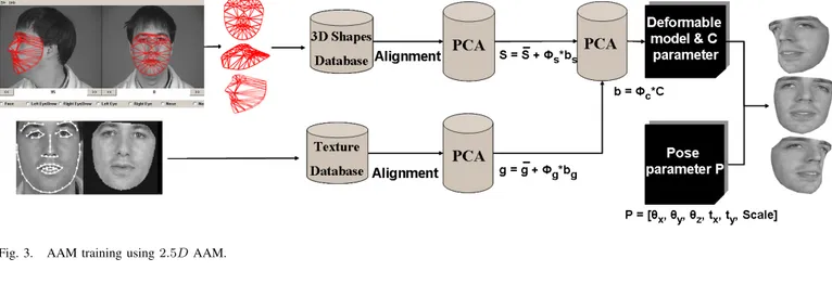
The training process of the 2.5D AAM is illustrated Fig. 3. For both sub-models, shapes are normalized using procrustes
JOURNAL OF LATEX CLASS FILES, VOL. 6, NO. 1, JANUARY 2007 5
Fig. 2. Landmarks for the eyes and mouth models.
analysis [50] and their means, called the mean shapes ¯s, are calculated. Principal Component Analysis (PCA) is performed on these shapes which results in the shape parameters with 95% of the variation represented by them. Thus, the eyes and mouth shapes can be synthesized by the equation:
si= ¯s + φs∗ bs (6)
where the matrix φs contains the eigenvectors of variation in
shapes and bsare the shape parameters.
All the textures of the eyes and mouth regions in the face images are warped (based on Delaunay triangulation) to the obtained mean shapes to form shape free patches and thus, their frontal views are extracted. Then, we calculate the mean of these textures ¯g. Another Principal Component Analysis (PCA) is performed on these textures to obtain the texture parameters, similarly with 95% of the variation stored in them. Hence, texture is synthesized by:
gi= ¯g + φg∗ bg (7)
where φg contains eigenvectors of variation in textures and
bg are the texture parameters. Parameters bs and bg are then
combined by concatenation as b = [bsbg]T and a final PCA is
performed to obtain the appearance parameters:
b = φc∗ C (8)
where φc are the eigenvectors and C is the vector of the
appearance parameters, which represent the shape and texture of the mouth or of the eyes of the facial image. Because we have a large training set, we have retained only 80% of the energy for the third PCA for both models. This has the advantage of reducing the computation time.
This 2.5D AAM can be translated as well as rotated with the help of the translational and rotational parameters forming the pose vector given as:
P = [θpitch, θyaw, θroll, tx, ty, Scale]T (9)
where θpitchcorresponds to the face rotating around the x axis
(head shaken up and down), θyaw to the face rotating around
y axis (head turned to profile views) and θroll to the face
rotating around the z axis (head doing circular rotations). tx
and ty represent the translation parameters from the supposed
origin and Scale controls the magnification of the model.
2) AAM searching: In the searching phase, the C and P parameters are varied to obtain an instance of the model (image synthesized by the model). This instance is placed on the face image to be segmented. The aim is to find the optimal vector of parameters which is the one that minimizes the pixel error E. E being the difference between the searched face image I(C, P ) and the one synthesized by the model M (C): E = ||I(C, P ) − M (C)|| (10) As an optimization scheme for determining the optimal vector of parameters, we use two consecutive Newton gradient descent algorithms. The difference between the two is that in the first one the learning of the relationship between the error and the displacement of the parameters is done offline during the training phase as proposed by Cootes [14], while in the second one we learn this relationship online. The obtained parameters from the first optimization scheme are entered into the second in order to refine the results. Figure 4 shows some results of our AAM fitting.
Fig. 4. AAM local models results on some test images showing successful eyes and mouth segmentation.
The disadvantage of a local model with respect to a global one is that in a global model the amount of error becomes relatively smaller in local areas having perturbations.
IV. CLASSIFIERS
To perform the AU recognition task, we have to make several binary decisions. Hence, we chose to train one Support Vector Machine (SVM) per AU. To train one SVM, all images containing the specific AU are used as positive samples (target class) and the other images are used as negatives (non-target class).
We have trained our detector to recognize AU (except AU25 and AU26) during speech sections as well as non-speech sections with the FERA sequences. Thus, the speech sections are treated like others during the test phase.
A. Multi-kernels SVMs
Given training samples composed of LGBP histograms and AAM coefficient vectors, xi= (Hi, Ci), associated with labels
yi(target or non-target), the classification function of the SVM
associates a score s to the new sample x = (H, C):
s = m X i=1 αik(xi, x) + b ! (11)
Fig. 3. AAM training using 2.5D AAM.
With αi the dual representation of the hyperplane’s normal
vector [51]. k is the kernel function resulting from the dot product in a transformed high-dimensional feature space.
In the case of multi-kernel SVM, the kernel k can be any convex combination of semi-definite functions.
k(xi, x) = K X j=1 βjkj with βj≥ 0, K X j=1 βj= 1 (12)
In our case, we have one kernel function per type of features. k = β1kLGBP(Hi, H) + β2kAAM(Ci, C) (13)
Weights αiand βjare set to have an optimum hyperplane in
the feature space induced by k. This hyperplane separates posi-tive and negaposi-tive classes and maximizes the margin (minimum distance of one sample to the hyperplane). This optimization problem has proven to be jointly-convex in αi and βj [52],
therefore there is a unique global minimum, which can be found efficiently.
β1 represents the weight accorded to the LGBP features
and β2 is the one for the AAM appearance vector. Thus,
using a learning database, the system is able to find the best combination of these two types of features that maximizes the margin.
This is a new way of using multi-kernel learning, instead of combining different kinds of kernel functions (for example Gaussian radial basis functions with polynomial functions), we combine different features.
The AAMs modelling approach takes the localization of the facial feature points into account and leads to a shape-free texture less-dependent to identity. But one of the severe drawbacks is the need of a good accuracy for the localization of the facial feature points. The GEMEP-FERA database contains large variations of expressions that sometimes lead to inaccurate facial landmarks tracking. In such cases, multi-kernel SVMs will decrease the importance given to AAM coefficients.
B. Kernel functions
In the section V, experimental results show that in histogram-based AU recognition, LGBP histograms are well-suited with the histogram intersection kernel:
KLGBP(Hi, Hj) =
X
k
min(Hi(k), Hj(k)) (14)
For the AAM appearance vectors, we use the Radial Basis Function (RBF) kernel :
KAAM(Ci, Cj) = e−
ksi−sj k2 2
2σ2 (15)
With σ a hyper-parameter we have to tune on a cross-validation database.
C. Temporal filtering
To take temporal information into account, we apply, for each AU, an average filter to the outputs of each SVM classifier of successive frames. The size of the average filter has been set to maximize the F1-measure reached on the training database.
Fig. 5 shows results obtained on one sequence using this approach. Table IV reports optimal filter size for each AU.
V. EXPERIMENTAL RESULTS WITH HISTOGRAM-BASED APPROACHES.
In this section we report previous experiments [53] per-formed on the Cohn-Kanade databases using a histogram-based approach. These previous results led us to choose the LGBP sequences and a histogram intersection kernel for the FERA challenge. We report the area under the ROC curve (2AFC) obtained in a leave-one-subject-out cross-validation process for 16 AUs: 7 upper face AUs (1, 2, 4 ,5, 6, 7 and 9) and 9 lower face AUs (11, 12, 15, 17, 20, 23, 24, 25 and 27). We compare different types of histograms, different methods to divide the image in blocks and different kernels used with an SVM classifier.
A. Features
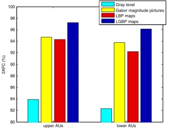
In Fig. 6, we compare the performance of different types of histograms using the histogram intersection kernel. The histograms computed from LBP maps and Gabor magnitude pictures perform much better than gray level histograms. The combination of both (LGBP) leads to the highest results.
JOURNAL OF LATEX CLASS FILES, VOL. 6, NO. 1, JANUARY 2007 7 0 10 20 30 −1 0 1 AU 1 0 10 20 30 −1 0 1 AU 2 0 10 20 30 −1 0 1 AU 4 0 10 20 30 −1 0 1 AU 6 0 10 20 30 −1 0 1 AU 7 0 10 20 30 −1 0 1 AU 10 0 10 20 30 −1 0 1 AU 12 0 10 20 30 −1 0 1 AU 15 0 10 20 30 −1 0 1 AU 17 0 10 20 30 −1 0 1 AU 18 Label SVM outputs
Detector binary outputs
Frame 5 Frame 9
Frame 21 Frame 25
Frame 13
Frame 17
Frame 5!
Frame 9!
Frame 13!
Frame 17!
Frame 21!
Frame 25!
Fig. 5. Signed and thresholded SVM outputs on one sequence of the GEMEP-FERA database.
upper AUs lower AUs
80 82 84 86 88 90 92 94 96 98 100 2AFC (%) Gray level
Gabor magnitude pictures LBP maps
LGBP maps
Fig. 6. Results on the Cohn-Kanade database, using different types of histograms with an SVM classifier and the histogram intersection kernel.
In Fig. 7, we compare the performance using different methods to divide the 128 × 128 image in block(s). We divide the image in n × n blocks, with n varying from 1 (full image, dimension is 1 × 6 × 3 × 256 = 768) to 6 (36 blocks, dimension is 36 × 6 × 3 × 256 = 165888). We can see that, for n lower or equal to 4, accuracy increases with n, then, it keeps quite stable. So we can say that 4x4 is a good trade of between accuracy (detection rate) and speed (dimensionality).
B. Kernel functions
Fig. 8 shows results performed with LGBP histograms and different kernels. For the polynomial and the RBF kernel, different values of the polynomial order and the standard deviation were tested. Experimental results are reported for the best parameter value. Though it results in over-fitting, it leads to lower performances than other kernels. Best results are reached with the histogram intersection kernel. Compared
upper AUs lower AUs
80 82 84 86 88 90 92 94 96 98 100 2AFC (%) 1x1 2x2 4x4 5x5 6x6
Fig. 7. Results on the Cohn-Kanade database, using different methods to divide the image in blocks.
to the linear kernel, the mean area under the ROC is increased from 95.5% to 97.2% and 93.0% to 96.1% for upper and lower AUs respectively. The RBF kernel leads to fair results but was directly tuned on the database.
C. Histogram reduction
Tab I shows the effect of different histogram reduction methods on the 2AFC performance. The 2AFC performance is not deteriorated when reducing the histogram bins number using the uniform patterns method or ours. However, our method results in a smaller histogram size than the uniform one. The rotational invariant patterns reduce the 2AFC score, this shows that an inappropriate regroupment of bins can decrease the performance of the AU detector.
upper AUs lower AUs 80 82 84 86 88 90 92 94 96 98 100 2AFC (%) Linear kernel
Third order polynomial kernel Gaussian kernel
Histogram intersection kernel
Fig. 8. Results on the Cohn-Kanade database, using LGBP histograms, an SVM classifier and different types of kernels.
Type of reduction bins per 2AFC(%) histogram upper lower None 256 97.2 96.0 This work (cf. III-A5) 26 97.2 96.1 Uniform patterns 58 97.3 96.1 Rotational invariant patterns 28 95.8 92.9
Uniform rotational
9 95.7 92.6 invariant patterns
TABLE I
2AFCON THECOHN-KANADE DATABASE FOR DIFFERENT HISTOGRAM
REDUCTION METHODS.
VI. EXPERIMENTS ON THEGEMEP-FERADATABASE
In this section we explain the training process of the AUs detector and report experiments on the GEMEP-FERA database. We used the training database of the challenge to study two points: (1) the interest of the fusion of two different types of features, (2) the use of different databases to recognize AUs.
A. Setup
1) Performance measurement: The F1-measure has been used to compare the participants’ results in the AU sub-challenge. The F1-measure considers both the precision p and the recall r of the test results to compute the score: p is the number of correct detections divided by the number of all returned detections and r is the number of correct detections divided by the number of detections that should have been returned. The F1-measure can be interpreted as a weighted average of the precision and recall, where an F1-measure reaches its best value at 1 and worst score at 0.
F = 2 · p · r
p + r (16)
To compute this measure, we need to threshold the outputs of our SVM classifiers. This is the major drawback of this measure, it is really dependent of the value of this threshold,
which explains why a naive system has performed better in terms of F1-measure than the baseline method of the organizer [37].
Hence, we chose to use a second measure that does not need the thresholding of the SVM outputs: the area under the ROC curve. By using the signed distance of each sample to the SVM hyper-plan and varying a decision threshold, we plot the hit rate (true positives) against the false alarm rate (false positives). The area under this curve is equivalent to the percentage of correct decisions in a 2-alternative forced choice task (2AFC), in which the system must choose which of the two images contains the target.
The 2AFC or area under the ROC curve is used to optimize the part of the system leading to unsigned values (SVM slack variable and the RBF kernel parameter). The F1-measure is used only to optimize the part of the system converting signed values to binary values (size of the average filter and thresholds).
2) Cross-Validation: For the experiments, the following databases are used as training databases:
• The Cohn-Kanade database [54]: the last image
(expres-sion apex) of all the 486 sequences. It contains images sequences of 97 university students ranging from ages of 18-30. The lighting conditions and context are relatively uniform and the images include small in-plane and out-plane head motion.
• The Bosphorus database [49]: around 500 images chosen because they exhibit a combination of two AUs. The lighting conditions and context are relatively uniform and the images include small in-plane and out-plane head motion.
• The GEMEP-FERA training dataset [12]: one frame from every sequence for every AU combination present resulting in 600 images.
The occurrence of each AU in these databases is reported Tab. III.
We use all the GEMEP-FERA training dataset as a cross-validation dataset to optimize the SVM slack-variable and, if needed, the RBF kernel parameter. We realize a 7-fold subject independent cross-validation. All the images of one subject from the GEMEP-FERA training dataset are used as a test set (around 800 images). Images of other subjects within the 600 selected from the GEMEP-FERA training dataset, and eventually from other databases, are used as a training dataset. After this cross-validation, to have 2AFC performances, we train the SVM classifiers with the optimized parameters on all the training dataset and apply them on the GEMEP-FERA test dataset for which we do not have the AU labels. Then, we send the signed outputs to the challenge organizers to have the 2AFC score.
To have the F1-measure performance, we merge the results of the 7-fold subject independent cross-validation. This leads to an SVM output for each AU and for each frame of the GEMEP-FERA training dataset. For each AU, we learn the size of the average filter and the decision threshold that lead to the best F1-measure. Using all these optimized parameters, we retrain the classifiers on all images, apply them on the
JOURNAL OF LATEX CLASS FILES, VOL. 6, NO. 1, JANUARY 2007 9
GEMEP-FERA test dataset and send the binary outputs to the challenge organizers to have the F1-measure.
B. Features and fusion strategies evaluation
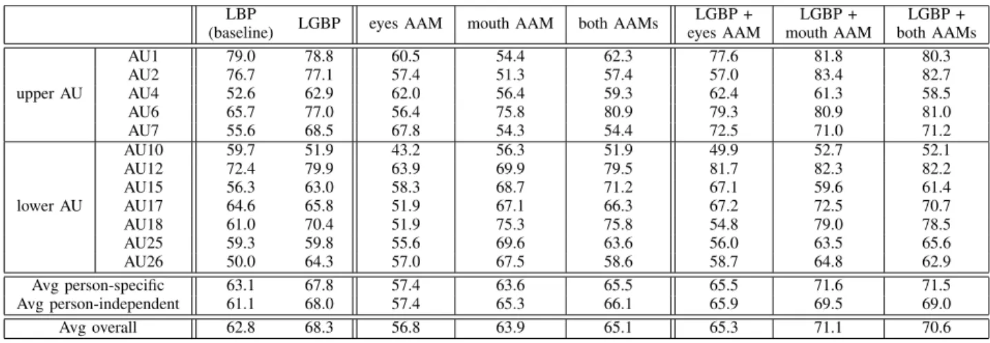
In this section, we train the system on the GEMEP-FERA training dataset, and report the 2AFC score on the GEMEP-FERA test dataset using different features and the fusion of features. After sending our signed outputs, organizers sent us 2AFC for each AU in 3 cases: person independent (test subjects are not in the training database), person specific (test subjects are in the training database) and overall. We report in Tab. II overall results for each AU and the average for the person specific, person independent and overall case.
Using only LGBP, we notice that we already have much bet-ter results than the baseline proposed by the organizers (68.3% against 62.8% overall). The two methods are really similar: equivalent setup, same training database, same classifier, only the features and the kernel function of the SVM are different. This confirms the results presented in section V.
Using only the AAM appearance vector, we notice that we have good results using the mouth AAM to detect the AUs localized in the lower part of the face. Results are even better than LGBP for the AUs 15, 17, 18, 25 and 26 (68.7% 67.1% 75.3% 69.6% and 67.5% against 63% 65.8% 70.4% 59.8% and 64.3% respectively). Results obtained for the upper part of the face are obviously not of a big importance (close to a random classifier’s response) using mouth information. Only the AU 6 is well detected, this is because this AU (cheek raiser) often appears with the AU12 (the smile). With eyes AAM, results are just slightly better than random classifiers (56.8% where a random system does 50%). This can be explained by the difficulty in fitting AAM with enough accuracy to detect AUs. The eyebrows, for example, are difficult to localize, especially when hair hides them.
Regarding the fusion, we notice that the eyes AAM does not increase performances if coupled with LGBP histograms. But the mouth AAM or both AAMs coupled with LGBPs lead to the best results. Surprisingly, the detection of the upper part face AUs is improved with the mouth AAM: 81.8%, 83.4%, 80.9% 71.0% for the AUs 1 2 6 and 7 respectively against 78.8% 77.1% 77.0% and 68.5% with LGBP only. As previously mentioned, the improvement for the AU 6 can be explained by the fact that this AU is related to the AU 12. However the improvement brought by the fusion for the other AUs is more difficult to interpret. The multi-kernel classifier may use the information given by the mouth AAM not to directly detect these upper part AUs, but to have information about the subject (for example, information about its identity, skin type...) that can help the classifier to better analyze LGBP features and increase the precision of the AUs detection using these LGBP features. This shows the interest of combining two types of different features.
Overall, the fusion of both AAMs with LGBP increases experimental results for 7 over 12 AUs, the AUs 1 2 6 7 12 17 and 18.
Finally, if we compare results in the person specific and person dependent cases, we notice that the fusion is better
than using only one feature type particularly in the person specific case.
C. AU labels transfer between databases
To evaluate the compatibility of AU labels between databases, we use the fusion of LGBP with AAM coefficients and train the system using different learning databases. We report in Tab. III experimental results on the GEMEP-FERA test dataset. We proceed to several tests using different combi-nations of the three different learning databases introduced in VI-A2. An enhanced learning database leads to better results: the system learned on the GEMEP-FERA and Cohn-Kanade databases and the system learned on the GEMEP-FERA and Bosphorus databases give better results than the system learned only on the GEMEP-FERA database (75.0%, and 73.7% respectively against 70.6%). However, adding the Bosphorus database to a training dataset already composed of the CK and the FERA decreases performances, as mixing databases may introduce too large variability in the AUs representation.
Test being on the GEMEP-FERA database, results using only the Cohn-Kanade and the Bosphorus databases are lower. Nevertheless, this last result highlights the good generalization ability of this framework.
Similar conclusions are reported in [19]. Without any re-training on FERA dataset, raw performances reached a 2AFC score of 72%. After retraining the whole system with all the datasets (including FERA), it reaches 76%.
A deeper study of Tab.III leads to the following conclusions: the first three trainings always include FERA database while the fourth one (CK and Bosphorus) exclude it. So, a possible explanation is that the greater variability induced by speech has been learnt by the system in the first three cases, leading to better generalizability on FERA test data. On the opposite, the fourth system is not able to generalize on speech sequences it has not seen during training.
D. Temporal filtering
To test the impact of the average filtering presented in section IV-C, we use the framework combining LGBP and AAM coefficients trained on the GEMEP-FERA and Cohn-Kanade databases. We report in Tab. IV, the filter size for each AU and the 2AFC scores using or not this filter.
We notice that the average filter significantly increases the 2AFC for all AUs.
E. Comparison on the test dataset with other methods For the challenge, we did not know these previous results computed on the GEMEP-FERA test dataset and so we could not use them to tune our system (for example by choosing the best databases combination to train each AU). We chose to use a fusion of LGBP and both AAMs coefficients and we trained the classifiers with the GEMEP-FERA, CK and Bosphorus databases for the AUs 1 2 4 12 15 17 and the GEMEP-FERA and CK databases for the other AUs. We chose not to use the Bosphorus database for the AUs that are not present in this database. The F1 scores obtained this way during the challenge
LBP LGBP eyes AAM mouth AAM both AAMs LGBP + LGBP + LGBP + (baseline) eyes AAM mouth AAM both AAMs upper AU AU1 79.0 78.8 60.5 54.4 62.3 77.6 81.8 80.3 AU2 76.7 77.1 57.4 51.3 57.4 57.0 83.4 82.7 AU4 52.6 62.9 62.0 56.4 59.3 62.4 61.3 58.5 AU6 65.7 77.0 56.4 75.8 80.9 79.3 80.9 81.0 AU7 55.6 68.5 67.8 54.3 54.4 72.5 71.0 71.2 lower AU AU10 59.7 51.9 43.2 56.3 51.9 49.9 52.7 52.1 AU12 72.4 79.9 63.9 69.9 79.5 81.7 82.3 82.2 AU15 56.3 63.0 58.3 68.7 71.2 67.1 59.6 61.4 AU17 64.6 65.8 51.9 67.1 66.3 67.2 72.5 70.7 AU18 61.0 70.4 51.9 75.3 75.8 54.8 79.0 78.5 AU25 59.3 59.8 55.6 69.6 63.6 56.0 63.5 65.6 AU26 50.0 64.3 57.0 67.5 58.6 58.7 64.8 62.9 Avg person-specific 63.1 67.8 57.4 63.6 65.5 65.5 71.6 71.5 Avg person-independent 61.1 68.0 57.4 65.3 66.1 65.9 69.5 69.0 Avg overall 62.8 68.3 56.8 63.9 65.1 65.3 71.1 70.6 TABLE II
2AFCSCORES ON THEGEMEP-FERATEST DATASET USINGLGBP,EYESAAMCOEFFICIENTS,MOUTHAAMCOEFFICIENTS,CONCATENATION OF THE
EYESAAMCOEFFICIENTS AND THE MOUTHAAMCOEFFICIENTS AND THE FUSION OFLGBPWITHAAMCOEFFICIENTS.
Number of samples Training databases
FERA CK Bos FERA FERA + CK FERA + Bos FERA + CK + Bos CK + Bos upper AU AU1 202 143 46 80.3 86.4 77.5 81.2 63.7 AU2 206 96 105 82.7 89.4 87.7 89.0 79.2 AU4 169 155 105 58.5 66.7 64.9 64.2 51.1 AU6 192 111 1 81.0 82.9 81.9 82.6 74.9 AU7 237 108 1 71.2 74.7 71.5 72.6 61.7 lower AU AU10 250 12 0 52.1 53.1 53.2 53.3 56.0 AU12 317 113 108 82.2 85.1 84.6 84.7 81.1 AU15 125 74 55 61.4 67.4 68.9 65.3 58.7 AU17 144 157 71 70.7 72.9 74.4 71.1 59.9 AU18 65 43 0 78.5 80.5 81.2 79.2 64.1 AU25 111 294 0 65.6 72.6 68.9 71.2 74.8 AU26 62 38 0 62.9 68.3 69.5 73.5 70.7 Avg person-specific 71.5 75.4 74.1 74.9 68.3 Avg person-independent 69.0 74.7 73.9 74.0 64.1 Avg overall 70.6 75.0 73.7 74.0 66.3 TABLE III
NUMBER OF SAMPLES IN EACH DATABASE AND2AFCSCORES ON THEGEMEP-FERATEST DATASET USING DIFFERENT TRAINING DATABASES.
Filter size No filtering Average filtering upper AU AU1 7 86.4 88.9 AU2 7 89.4 91.4 AU4 5 66.7 68.0 AU6 7 82.9 84.9 AU7 5 74.7 76.1 lower AU AU10 7 53.1 53.7 AU12 7 85.1 86.3 AU15 7 67.4 70.0 AU17 3 72.9 74.7 AU18 3 80.5 81.9 AU25 5 72.6 73.6 AU26 5 68.3 71.2 Avg person-specific 75.4 77.0 Avg person-independent 74.7 76.6 Avg overall 75.0 76.7 TABLE IV
FILTER SIZE(NUMBER OF SUCCESSIVE FRAMES TAKEN INTO ACCOUNT)
AND2AFCSCORES ON THEGEMEP-FERATEST DATASET USING OR
NOT AN AVERAGE FILTER ON THESVMOUTPUTS.
0 10 20 30 40 50 60 70 Baseline MIT-‐Cambridge QUT KIT UCSD This work Person Specific Person independent
Fig. 9. FERA challenge official F1 results of all participants. UCSD: University of San Diego [19]. KIT: Karlsruhe Institute of Technology. QUT: Queensland University of Technology [45]. MIT-Cambride : Massachusetts Institute of Technology and University of Cambridge [46].
and those of all participants are reported in Fig. 9. The system described in this article outperformed all other systems in the person independent and in the person specific case.
A synthesis of the different results presented in this article and a comparison of the different methods of each participant
JOURNAL OF LATEX CLASS FILES, VOL. 6, NO. 1, JANUARY 2007 11
Participants Type Features Classifiers Learning database F1 2AFC 1-Baseline[37] A, F LBP histograms + PCA SVM G 0.45 0.63 2-Baltrusaitis et al.[46] G+A, T Tracked landmark + Gabor filters Rule based + SVM G 0.46 3-Chew et al.[45] G, T Constrained Local Models SVM G+CK 0.51 4a-Wu et al.[19] A, F Gabor filters AdaBoost + SVM G + CK + MMI + pr 0.55 0.72 4b A, C Gabor filters AdaBoost + SVM G + CK + MMI + pr 0.58 0.76 5a-This work A, F LGBP histogram SVM G 0.68
5b G+A, F AAM SVM G 0.65
5c G+A, F LGBP histogram + AAM MKL SVM G + CK + Bos 0.75 5d G+A, C LGBP histogram + AAM MKL SVM G + CK + Bos 0.62 0.77
TABLE V
PARTICIPANT SUMMARY TABLE EXPOSINGNG THE DIFFERENT TYPES OF APPROACHES- G/A : GEOMETRIC/APPEARANCE. F/T/C :
FRAME-BY-FRAME/TRACKING/CONTEXT. G/CK/MMI/BOS/PR: GEMEP-FERA, COHN-KANADE, MMI, BOSPHORUS AND PRIVATE DATABASE.
is summarized in Tab. V.
First, let us compare purely appearance-based approaches. Participant 1 used LBP histograms (reduced by PCA) and SVM with RBF kernel, 5a used LGBP histogram and SVM with histogram intersection kernel. The increasing accuracy (from 62.8 to 68.3) can easily be explained by a slight superiority of Gabor encoding (also reported in [19]) over LBP and, last but not least, a kernel function well-suited to the feature it has to deal with. Participant 3 should be compared with participant 5 second experiment (5b). The first uses CLM, the second one, AAM. They take advantages of both geomet-rical and local appearance information. Unfortunately, as the training dataset and the performance measure are different, we cannot fairly compare results. Anyway, these experiments show lower accuracy than previous purely appearance-based methods. These results are only outperformed when participant 5 in his third experiment (5c) combines spatial-independent appearance features (LGBP) with geometric and local ap-pearance information (AAM) with the help of Multi-Kernel SVMs. Finally, we can notice that taking into account the temporal sequence context improve overall accuracy as shown in Participant 4 experiments (from 72.3 to 75.8) as well as participant 5 fourth experiment (from 75.0% to 76.7%).
VII. EMOTION RECOGNITION RESULTS
In this section, we also evaluate our framework for emotion detection which corresponds to the second task of the FERA challenge. The objective is to assess the relevance of our framework to deal with a different kind of data. In fact, information of the emotion is more spread over the entire face and it involves a higher level of interpretation.
The objective of emotion detection task is to label each sequence with one of the five discrete emotion classes: Anger, Fear, Joy, Relief and Sadness. This task differs from the pre-vious task in that the decision is made for the entire sequence, contrary to the previous frame by frame AU detection. In addition, this classification problem corresponds to a 5-class forced choice problem. So, we have to slightly adapt our framework in order to match these constraints. We adopt a straightforward strategy similar to that proposed by [37]. For the training step, we consider that all images of a sequence are equally informative. So we keep one quarter of the images uniformly distributed over the sequence in order to train our one-against-all multi-class SVM. During testing, we apply our
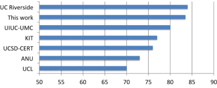
50# 55# 60# 65# 70# 75# 80# 85# 90# UCL# ANU# UCSD/CERT# KIT# UIUC/UMC# This#work# UC#Riverside#
Fig. 10. Comparison of our method emotion classification rate with results of the FERA emotion sub-challenge.
detector on every frame of the sequence and the emotion label which occurred in the largest number of frame is assigned to the sequence.
Classification rates we obtained for the emotion detection sub-challenge are reported in table VI. The overall results are compared with those obtained by the participants of the FERA emotion sub-challenge and shown in Fig. 10. We can notice that our method obtains the second best result for this task.
PI PS Overall Anger 92.9 100 96.3 Fear 46.7 90.0 64.0 Joy 95.0 100 96.8 Relief 75.0 100 84.6 Sadness 60.0 100 76.0 Avg. 73.9 98.0 83.5 TABLE VI
CLASSIFICATION RATES FOR EMOTION RECOGNITION ON THE TEST SET
FOR OUR METHOD. PERFORMANCE IS SHOWN FOR THE PERSON
INDEPENDENT(PI),PERSON SPECIFIC(PS)AND OVERALL PARTITION.
VIII. CONCLUSION
We have proposed here an original framework to perform action unit detection. We combine spatial-independent feature extraction (LGBP histograms) and statistical spatial shape and texture information (AAM coefficients). To deal with these two kinds of information and take the best of both, we propose to use advanced learning machine algorithms. Multi-kernel SVMs can help in selecting the most accurate information as each kernel function is weighted depending on this latter.
Experimental results in independent and person-specific setups show that LGBP histograms perform better than AAM. We had difficulties in fitting AAMs on expressive faces with enough accuracy to detect AUs, specifically in the upper part of the face. But even with inaccurate AAMs, the combination of features increases the area under the ROC curve of 9 over 12 AUs. Experiments using different learning databases show the limited compatibility of AU labels between databases.
Finally, F1 results obtained with this system were the best among all participants showing the good performance of the chosen approach. This success can be explained by the following points:
• The good overall generalization ability of LGBP his-tograms coupled with an intersection histogram kernel.
• The use of multi-kernel learning to fuse features. • The optimization of the 2AFC score first and then the F1
measure during the cross-validation process.
• The use of several training databases. Even if our choice
was not optimal, as using only the FERA-GEMEP database and the Cohn-Kanade database would have led us to better results.
But overall results remain insufficient, some AUs are de-tected with an accuracy just slightly better than their detection with a random system. There is still room for improvement. Like most of the participants, we detect AUs frame by frame, using static classifiers. To exploit the temporal component of the sequences, we only use an average filter on the SVM outputs. We believe that experimental results could be signifi-cantly increased by finding segments in a sequence containing the start and the end of the AU.
ACKNOWLEDGMENT
This work has been partially supported by the French National Agency (ANR) in the frame of its Technological Research CONTINT program (IMMEMO, project number ANR-09-CORD-012) and the Cap Digital Business cluster for digital content.
REFERENCES
[1] A. Mehrabian and M. Wiener, “Decoding of inconsistent communica-tions,” Journal of Personality and Social Psychology, vol. 6, no. 1, pp. 109–114, 1967.
[2] N. Ambady and R. Rosenthal, “Thin slices of expressive behavior as pre-dictors of interpersonal consequences: A meta-analysis,” Psychological bulletin, vol. 111, no. 2, pp. 256–274, 03 1992.
[3] J. Russell and J. Dols, The psychology of facial expression, ser. Studies in emotion and social interaction. Cambridge University Press, 1997. [Online]. Available: http://books.google.fr/books?id=rr8e5oMlj44C [4] M. Knapp and J. Hall, Nonverbal communication in human interaction,
4th ed. Harcourt College Pub, 1996.
[5] M. Pantic, Face for Ambient Interface. Springer, 2006, vol. 3864, pp. 35–66.
[6] D. Keltner and P. Ekman, Facial expression of emotion. Guilford Publications, 2000.
[7] K. Scherer, “What are emotions? and how can they be measured?” Social science information, vol. 44, no. 4, pp. 695–729, 2005.
[8] P. Ekman and W. Friesen, “Facial action coding system (facs): A tech-nique for the measurement of facial actions,” Consulting Psychologists Press, 1978.
[9] M. Pantic and L. Rothkrantz, “Expert system for automatic analysis of facial expressions,” Image and Vision Computing, vol. 18, no. 11, pp. 881–905, 2000.
[10] P. Phillips, P. Flynn, T. Scruggs, K. Bowyer, J. Chang, K. Hoffman, J. Marques, J. Min, and W. Worek, “Overview of the face recognition grand challenge,” in Proc. IEEE Int’l Conf. Computer Vision and Pattern Recognition (CVPR ’05), 2005.
[11] P. Phillips, H. Moon, P. Rauss, and S. Rizvi, “The feret evaluation methodology for face-recognition algorithms,” in IEEE Trans. on Pattern Analysis and Machine Intelligence, 2000.
[12] T. Banziger and K. R. Scherer, “Using actor portrayals to systematically study multimodal emotion expression: The gemep corpus,” p. 476, 2007. [13] W. Zhang, S. Shan, W. Gao, X. Chen, and H. Zhang, “Lgbphs: A novel non-statistical model for face representation and recognition,” in Proc. IEEE Int’l Conf. on Computer Vision (ICCV ’05), 2005.
[14] T. Cootes, G. Edwards, and C. Taylor, “Active appearance models,” in Proc. IEEE European Conf. on Computer Vision (ECCV ’98). Springer, 1998, p. 484.
[15] A. Rakotomamonjy, F. Bach, S. Canu, and Y. Grandvalet, “SimpleMKL,” Journal of Machine Learning Research, vol. 9, pp. 2491–2521, 2008. [16] Y. Zhu, F. De la Torre, J. Cohn, and Y.-J. Zhang, “Dynamic cascades with
bidirectional bootstrapping for spontaneous facial action unit detection.” in Proc. of Affective Computing and Intelligent Interaction (ACII’09), 2009.
[17] P. Viola and M. Jones, “Robust real-time face detection,” Int’l Journal of Computer Vision, vol. 57, no. 2, pp. 137–154, 2004.
[18] M. Eckhardt, I. Fasel, and J. Movellan, “Towards practical facial feature detection,” Int’l Journal of Pattern Recognition and Artificial Intelligence, 2009.
[19] T. Wu, N. Butko, P. Ruvolo, J. Whitehill, M. Bartlett, and J. Movellan, “Action unit recognition transfer across datasets,” in Proc. IEEE FG’11, Facial Expression Recognition and Analysis Challenge (FERA’11), 2011.
[20] V. Rapp, T. Senechal, K. Bailly, and L. Prevost, “Multiple kernel learning svm and statistical validation for facial landmark detection,” in Proc. IEEE Int’l. Conf. Face and Gesture Recognition (FG’11), 2011. [21] I. Kotsia and I. Pitas, “Facial expression recognition in image sequences
using geometric deformation features and support vector machines,” IEEE Trans. on Image Processing, vol. 16, no. 1, pp. 172–187, 2007. [22] A. Asthana, J. Saragih, M. Wagner, and R. Goecke, “Evaluating aam
fitting methods for facial expression recognition,” in Proc. Third Int’l Conf. on Affective Computing and Intelligent Interaction (ACII ’09), 2009.
[23] J. Saragih, S. Lucey, and J. Cohn, “Face alignment through subspace constrained mean-shifts,” in Proc. IEEE Int’l Conf. on Computer Vision (ICCV ’09). IEEE, 2009, pp. 1034–1041.
[24] Z. Wen and T. Huang, “Capturing subtle facial motions in 3d face tracking,” in Proc. IEEE Int’l Conf. on Computer Vision (ICCV ’03), 2003, pp. 1343–1350.
[25] J. Cohn, L. Reed, Z. Ambadar, J. Xiao, and T. Moriyama, “Automatic analysis and recognition of brow actions and head motion in sponta-neous facial behavior,” in Proc. IEEE Int’l Conf. Systems, Man, and Cybernetics (SMC ’04), vol. 1, 2004, pp. 610–616.
[26] Z. Zeng, M. Pantic, G. Roisman, and T. Huang, “A survey of affect recognition methods: Audio, visual, and spontaneous expressions,” IEEE Trans. on Pattern Analysis and Machine Intelligence, vol. 31, no. 1, pp. 39–58, 2009.
[27] M. Valstar and M. Pantic, “Fully automatic facial action unit detection and temporal analysis,” in Proc. IEEE Int’l Conf. Computer Vision and Pattern Recognition (CVPR ’06), 2006.
[28] I. Cohen, N. Sebe, A. Garg, L. Chen, and T. Huang, “Facial expression recognition from video sequences: Temporal and static modeling,” Computer Vision and Image Understanding, vol. 91, no. 1-2, pp. 160– 187, 2003.
[29] N. Sebe, M. Lew, Y. Sun, I. Cohen, T. Gevers, and T. Huang, “Authentic facial expression analysis,” Image and Vision Computing, vol. 25, no. 12, pp. 1856–1863, 2007.
[30] M. Bartlett, G. Littlewort, M. Frank, I. Fasel, and J. Movellan, “Auto-matic recognition of facial actions in spontaneous expressions,” Journal of Multimedia, 2006.
[31] J. Bazzo and M. Lamar, “Recognizing facial actions using gabor wavelets with neutral face average difference,” in Proc. IEEE Int’l Conf. Automatic Face and Gesture Recognition (AFGR ’04), 2004, pp. 505– 510.
[32] Y. Tong, W. Liao, and Q. Ji, “Facial action unit recognition by exploiting their dynamic and semantic relationships,” IEEE Trans. on Pattern Analysis and Machine Intelligence, vol. 29, no. 10, pp. 1683–1699, 2007. [33] J. Whitehill and C. Omlin, “Haar features for facs au recognition,” in Proc. IEEE Int’l Conf. Automatic Face and Gesture Recognition (AFGR ’06), 2006, p. 5.
JOURNAL OF LATEX CLASS FILES, VOL. 6, NO. 1, JANUARY 2007 13
[34] C. Chuang and F. Shih, “Recognizing facial action units using in-dependent component analysis and support vector machine,” Pattern recognition, vol. 39, no. 9, pp. 1795–1798, 2006.
[35] S. Moore, R. Bowden, and U. Guildford, “The effects of pose on facial expression recognition,” in Proc. British Machine Vision Conf. (BMVC ’09), 2009.
[36] B. Fasel, F. Monay, and D. Gatica-Perez, “Latent semantic analysis of facial action codes for automatic facial expression recognition,” in Proc. Sixth ACM Int’l Workshop Multimedia Information Retrieval (MIR ’04). ACM, 2004, pp. 181–188.
[37] M. Valstar, B. Jiang, M. M´ehu, M. Pantic, and K. Scherer, “The first facial expression recognition and analysis challenge,” in IEEE Int’l. Conf. Face and Gesture Recognition (FG’11), 2011.
[38] I. Essa and A. Pentland, “Coding, analysis, interpretation, and recogni-tion of facial expressions,” IEEE Trans. on Pattern Analysis and Machine Intelligence, pp. 757–763, 1997.
[39] M. Valstar, M. Pantic, and I. Patras, “Motion history for facial action detection in video,” in Proc. IEEE Int’l Conf. Systems, Man, and Cybernetics (SMC ’04), vol. 1, 2004.
[40] S. Koelstra, M. Pantic, and I. Patras, “A dynamic texture based approach to recognition of facial actions and their temporal models,” IEEE Trans. on Pattern Analysis and Machine Intelligence, 2010.
[41] D. Chetverikov and R. P´eteri, “A brief survey of dynamic texture description and recognition,” Computer Recognition Systems, pp. 17– 26, 2005.
[42] G. Zhao and M. Pietikainen, “Dynamic texture recognition using local binary patterns with an application to facial expressions,” IEEE Trans-actions on Pattern Analysis and Machine Intelligence, vol. 29, no. 6, pp. 915–928, 2007.
[43] Y. Tian, T. Kanade, and J. Cohn, Handbook of Face Recognition. Springer, 2005, ch. Facial Expression Analysis, pp. 247–276. [44] Y. Zhang and Q. Ji, “Active and dynamic information fusion for
facial expression understanding from image sequences,” IEEE Trans. on Pattern Analysis and Machine Intelligence, vol. 27, no. 5, pp. 699–714, 2005.
[45] S. Chew, P. Lucey, S. Lucey, J. Saragih, J. Cohn, and S. Sridharan, “Person-independent facial expression detection using constrained local models,” in Proc. IEEE FG’11, Facial Expression Recognition and Analysis Challenge (FERA’11), 2011.
[46] T. Baltrusaitis, D. McDuff, N. Banda, M. Mahmoud, R. Kaliouby, P. Robinson, and R. Picard, “Real-time inference of mental states from facial expressions and upper body gestures,” in Proc. IEEE FG’11, Facial Expression Recognition and Analysis Challenge (FERA’11), 2011.
[47] T. Ojala, M. Pietikainen, and D. Harwood, “A comparative study of texture measures with classification based on featured distributions,” Pattern Recognition, vol. 29, no. 1, pp. 51–59, 1996.
[48] A. Sattar, Y. Aidarous, S. Le Gallou, and R. Seguier, “Face alignment by 2.5 d active appearance model optimized by simplex,” in Proc. Int’l Conf. on Computer Vision Systems (ICVS’07), 2007.
[49] A. Savran, N. Alyuz, H. Dibeklioglu, O. Celiktutan, B. Gokberk, B. Sankur, and L. Akarun, “Bosphorus database for 3d face analysis,” Biometrics and Identity Management, pp. 47–56, 2008.
[50] A. Ross, “Procrustes analysis,” Course report, Department of Computer Science and Engineering, University of South Carolina, 2004. [51] B. Scholkopf and A. Smola, Learning with Kernels. MIT Presss, 2002. [52] G. Lanckriet, N. Cristianini, P. Bartlett, L. Ghaoui, and M. Jordan, “Learning the kernel matrix with semidefinite programming,” The Jour-nal of Machine Learning Research, vol. 5, p. 27, 2004.
[53] T. Senechal, K. Bailly, and L. Prevost, “Automatic facial action detection using histogram variation between emotional states,” in Proc. Int’l Conf. Pattern Recognition (ICPR’10), 2010.
[54] T. Kanade, J. Cohn, and Y. Tian, “Comprehensive database for facial expression analysis,” in Proc. IEEE Int’l Conf. Automatic Face and Gesture Recognition (AFGR ’00), 2000, pp. 46–53.
Thibaud Senechal received the M.Sc. Degree from Pierre et Marie Curie university, Paris, France, in 2008. He defended his Ph.D degree in 2011 in the ISIR lab, Pierre et Marie Curie university, Paris, France. His research interests include machine learn-ing, pattern recognition, computer vision, automatic facial expression recognition and facial action cod-ing. He is currently working for Affectiva as a re-search scientist, developing algorithms to recognize facial expressions from sequences. In 2011, he was the recipient of the best entry award in the first international facial expression recognition challenge, FERA, at the Face and Gesture 2011 conference, Santa Barbara.
Vincent Rapp is currently pursuing the Ph.D degree in Computer Science at the Institute of Intelligent Systems and Robotics (ISIR), University Pierre and Marie Curie (UPMC), Paris, France. He received the B.Sc and M.Sc degrees in Electrical Engineering from the UPMC in 2007 and 2009, respectively. His research interests are in pattern recognition and machine learning techniques, focusing on face analysis applications.
Hanan Salam received the B.Eng in Electrical and Computer engineering from the Lebanese University, Beyrouth, Lebanon, and the M.Eng in Signal and Image processing from the Ecole Centrale, Nantes, France in 2010. She is currently working to get her Ph.D degree at the SCEE (Communication and Elec-tronic Embedded Systems) lab of Suplec, Rennes, France. Her research interests include face analysis and eye gaze detection for Human-Machine Inter-face.
Renaud Seguier Renaud Seguier received the Ph.D degrees in Signal Processing, Image, Radar from the University of Rennes I in 1995 and the HDR (Habil-itation Diriger des Recherches) in 2012. He worked one year in Philips R&D department on numerical TV and Mpeg2 transport-stream. He joined SCEE (Communication and Electronic Embedded Systems) lab of Suplec in 1997 since when he is Assistant Professor and now Professor in Image Processing, Artificial Life and Numerical Implementation. His current research focuses on face analysis and synthe-sis for object video-compression and Human-Machine Interface. He is now involved in several collaborative projects for which he works on real-time human expression recognition and learning throw video sensors. He is a co-founder of Dynamixyz, a company specialized in face analysis and synthesis for video games industry and animation movies.
Kevin Bailly is an Associate Professor at the In-stitute of Intelligent Systems and Robotics (ISIR), University Pierre and Marie Curie (UPMC), Paris, France. He received the Engineering degree from the IMAC Graduate Engineering School (2003) and the Masters degree from University of Paris-Est (2004). He earned the Ph.D. degree in Computer Science from UPMC (2010). His main areas of research are machine learning and computer vision applied to face processing and automatic behavior analysis.
Lionel Prevost defended his Ph.D Thesis on com-puter science in 1998 and his supervision Degree in 2007, at Pierre and Marie Curie University, Paris, France. He was Assistant Professor at the Institute of Intelligent Systems and Robotics till 2010. Then, he joined as Full Professor the University of French West Indies and Guiana, Pointe--Pitre, France. His research interests are pattern recognition, machine learning and information fusion. He supervised sev-eral PhDs on handwritten text recognition, object detection and face analysis. He is now involved in several collaborative projects focusing on face localization and emotion recognition in still images and videos. He published more than 50 papers in international journals and forefront conferences. He is program committee member for a number of conferences and chaired the 3rd International Workshop on Artificial Neural Networks in Pattern Recognition he organized in Paris in 2008