HAL Id: tel-02955821
https://tel.archives-ouvertes.fr/tel-02955821
Submitted on 2 Oct 2020HAL is a multi-disciplinary open access
archive for the deposit and dissemination of sci-entific research documents, whether they are pub-lished or not. The documents may come from teaching and research institutions in France or abroad, or from public or private research centers.
L’archive ouverte pluridisciplinaire HAL, est destinée au dépôt et à la diffusion de documents scientifiques de niveau recherche, publiés ou non, émanant des établissements d’enseignement et de recherche français ou étrangers, des laboratoires publics ou privés.
of continuum medium aiming image-based diagnostics
Romain Noel
To cite this version:
Romain Noel. The lattice Boltzmann method for numerical simulation of continuum medium aiming image-based diagnostics. Other. Université de Lyon, 2019. English. �NNT : 2019LYSEM015�. �tel-02955821�
N
◦d’ordre NNT: 2019LYSEM015
THÈSE de DOCTORAT DE L’UNIVERSITÉ DE LYON
opérée au sein de
École des Mines de Saint-Étienne
École Doctorale N
◦488
(Sciences, Ingénierie, Santé)
Spécialité de doctorat: Mathématiques et leurs interactions
Discipline: Physique Computationnelle
Soutenue publiquement le 28/06/2019, par:
Romain
Noël
La méthode de Boltzmann sur réseau pour la simulation
numérique des milieux continus en vue de diagnostics à partir
d’images
—
The lattice Boltzmann method for numerical simulation of
continuum medium aiming image-based diagnostics
Devant le jury composé de:
Lamarque, Claude-Henri Professeur ENTPE Président du Jury Chen, Yu Professeur associé Yancheng Teachers University Rapporteur Clausel, Marianne Professeure Université de Lorraine Rapporteur Fournel, Thierry Professeur Université Jean Monnet Examinateur
Courbebaisse, Guy Ingénieur de Recherche INSA Lyon Co-directeur de thèse Navarro, Laurent Chargé de Recherche Mines Saint-Étienne Directeur de thèse
SCIENCES DE LA TERRE B. Guy , Directeur de recherche SCIENCES ET GENIE DE L’ENVIRONNEMENT D. Graillot, Directeur de recherche
GENIE INDUSTRIEL N. Absi, Maitre de recherche MICROELECTRONIQUE Ph. Lalevée, Professeur
EMSE : Ense ignants-chercheurs e t chercheurs autorisés à diriger de s thèses de doctorat (titulaires d’un doctorat d’État ou d’une HDR)
ABSI Nabil MR Génie industriel CMP
AUGUSTO Vincent CR Im age, Vision, Signal CIS
AVRIL Stéphane PR2 Mécanique et ingénierie CIS
BADEL Pierre MA(MDC) Mécanique et ingénierie CIS
BALBO Flavien PR2 Inform atique FAYOL
BASSEREAU Jean-François PR Sciences et génie des matériaux SMS
BATTON-HUBERT Mireille PR2 Sciences et génie de l'environnement FAYOL
BEIGBEDER Michel MA(MDC) Inform atique FAYOL
BLAYAC Sy lvain MA(MDC) Microélectronique CMP
BOISSIER Olivier PR1 Inform atique FAYOL
BONNEFOY Olivier PR Génie des Procédés SPIN
BORBELY Andras MR(DR2) Sciences et génie des matériaux SMS
BOUCHER Xavier PR2 Génie Industriel FAYOL
BRODHAG Christian DR Sciences et génie de l'environnement FAYOL
BRUCHON Julien MA(MDC) Mécanique et ingénierie SMS
CAMEIRAO Ana MA(MDC) Génie des Procédés SPIN
CHRISTIEN Frédéric PR Science et génie des matériaux SMS
DAUZERE-PERES Stéphane PR1 Génie Industriel CMP
DEBAYLE Johan MR Sciences des Images et des Formes SPIN
DEGEORGE Jean-Michel MA(MDC) Génie industriel Fay ol
DELAFOSSE David PR0 Sciences et génie des matériaux SMS
DELORME Xavier MA(MDC) Génie industriel FAYOL
DESRAYAUD Christophe PR1 Mécanique et ingénierie SMS
DJENIZIAN Thierry PR Science et génie des matériaux CMP
BERGER-DOUCE Sandrine PR1 Sciences de gestion FAYOL
DRAPIER Sy lvain PR1 Mécanique et ingénierie SMS
DUTERTRE Jean-Max MA(MDC) CMP
EL MRABET Nadia MA(MDC) CMP
FAUCHEU Jenny MA(MDC) Sciences et génie des matériaux SMS
FAVERGEON Loïc CR Génie des Procédés SPIN
FEILLET Dom inique PR1 Génie Industriel CMP
FOREST Valérie MA(MDC) Génie des Procédés CIS
FRACZKIEWICZ Anna DR Sciences et génie des matériaux SMS
GARCIA Daniel MR(DR2) Sciences de la Terre SPIN
GAVET Yann MA(MDC) Sciences des Images et des Formes SPIN
GERINGER Jean MA(MDC) Sciences et génie des matériaux CIS
GOEURIOT Dom inique DR Sciences et génie des matériaux SMS
GONDRAN Natacha MA(MDC) Sciences et génie de l'environnement FAYOL
GONZALEZ FELIU Jesus MA(MDC) Sciences économiques FAYOL
GRAILLOT Didier DR Sciences et génie de l'environnement SPIN
GROSSEAU Philippe DR Génie des Procédés SPIN
GRUY Frédéric PR1 Génie des Procédés SPIN
HAN Woo-Suck MR Mécanique et ingénierie SMS
HERRI Jean Michel PR1 Génie des Procédés SPIN
KERMOUCHE Guillaum e PR2 Mécanique et Ingénierie SMS
KLOCKER Helm ut DR Sciences et génie des matériaux SMS
LAFOREST Valérie MR(DR2) Sciences et génie de l'environnement FAYOL
LERICHE Rodolphe CR Mécanique et ingénierie FAYOL
MALLIARAS Georges PR1 Microélectronique CMP
MOLIMARD Jérôm e PR2 Mécanique et ingénierie CIS
MOUTTE Jacques CR Génie des Procédés SPIN
NAVARRO Laurent CR CIS
NEUBERT Gilles FAYOL
NIKOLOVSKI Jean-Pierre Ingénieur de recherche Mécanique et ingénierie CMP
NORTIER Patrice PR1 Génie des Procédés SPIN
O CONNOR Rodney Philip MA(MDC) Microélectronique CMP
PICARD Gauthier MA(MDC) Inform atique FAYOL
PINOLI Jean Charles PR0 Sciences des Images et des Formes SPIN
POURCHEZ Jérém y MR Génie des Procédés CIS
ROUSSY Agnès MA(MDC) Microélectronique CMP
ROUSTANT Olivier MA(MDC) Mathém atiques appliquées FAYOL
SANAUR Sébastien MA(MDC) Microélectronique CMP
SERRIS Eric IRD FAYOL
STOLARZ Jacques CR Sciences et génie des matériaux SMS
TRIA Assia Ingénieur de recherche Microélectronique CMP
VALDIVIESO François PR2 Sciences et génie des matériaux SMS
VIRICELLE Jean Paul DR Génie des Procédés SPIN
WOLSKI Krzy stof DR Sciences et génie des matériaux SMS
XIE Xiaolan PR0 Génie industriel CIS
YUGMA Gallian CR Génie industriel CMP
M is e à jo u r : 3 0 /0 8 /2 0 18
Ph.D. Thesis
The lattice Boltzmann method for numerical simulation of continuum
medium aiming image-based diagnostics
Abstract
Abstract
To determine the evolution in time of existing bodies, it is necessary to start from a given confi and perform predictive computations. To obtain information from within the matter without destroying it, is not an easy task. When degradation is not possible, a common way to acquire the initial configuration is the use of imaging systems. And due to the complexity of the behaviour of matter, it is also common to resort to numerical methods in order to simulate these temporal processes. A relatively recent numerical method called Lattice Boltzmann Method (LBM) tackles the evolution process at a mesoscopic scale. The combination of these two fields is originally investigated in this thesis, around the use of the LBM for numerical simulations of continuum medium aiming image-based diagnostics.
Foremost, an extension of the LBM to the morphological mathematics is suggested. It contributes to the development of a new concept: the coupling of image processing, mechanical and biological simulations on a single network. Then, the simulation of solids with LBM is addressed, using two different approaches. The first one provides an analytical Multiple Relaxation Times methods to generate arbitrary stress tensor and heat flux. The second introduces the divergence of the stress tensor into the Vlasov equation. Both approaches are numerically confronted with theoretical results in 1D and 2D and offer promising perspectives.
Résumé
Pour déterminer l’évolution temporelle de corps existants, il est nécessaire de partir d’une confi donnée et d’effectuer des calculs prédictifs. Obtenir des informations de l’intérieur de la matière sans la détruire, n’est pas une tâche facile. Lorsque la dégradation n’est pas possible, un moyen courant d’acquérir la confi de départ est l’utilisation de systèmes d’imageries. Et en raison de la complexité du comportement de la matière, il est également courant de recourir à des méthodes numériques pour simuler les processus temporels. Une méthode numérique relativement récente appelée méthode de Boltzmann
sur réseau (LBM) permet d’aborder le processus d’évolution à une échelle mésoscopique.
La combinaison de ces deux domaines est étudiée de manière originale dans cette thèse, autour de l’utilisation de la LBM pour les simulations numériques des milieux continus en vue de diagnostics à partir d’images.
Tout d’abord, une extension de la LBM à la morphologie mathématique est proposée. Elle concourt au développement d’un nouveau concept: le couplage du traitement d’images, des simulations mécaniques et biologiques sur un seul réseau. Ensuite, la simulation des solides avec la LBM est abordée, via deux approches différentes. La première fournit une méthode à multiples temps de relaxation analytique pour générer un tenseur de contrainte et un flux de chaleur arbitraires. La seconde introduit la divergence du tenseur de contrainte dans l’équation de Vlasov. Les deux approches sont confrontées numériquement à des résultats théoriques en 1D et 2D et offrent des perspectives prometteuses.
Dédicace
Remerciements
Je tiens ici à remercier toutes les personnes qui ont apporté, à leurs manières, leurs soutiens et contributions à cette thèse. J’ai conscience de la chance que j’ai, car ils sont nombreux. Pour autant, ils ne me rendent pas la tâche si aisée, car il ne faut oublier personne. Je vais essayer.Je suis en premier lieu très reconnaissant aux membres du jury : leur validation est un élément rassurant et confortant mes choix. Merci à Thierry Fournel d’avoir accepté rapidement de participer à ce jury et pour ses questions pertinentes. Je souhaite remercier les rapporteurs Yu Chen et Marianne Clausel d’avoir examiné mes travaux, lu attenti- vement ce manuscrit et formulé des critiques constructives. Je voudrais bien sûr exprimer ma gratitude au président du jury Claude-Henri Lamarque pour la confi et le sou- tien qu’il m’apporte depuis plusieurs années, ainsi que ses remarques, questionnements et conseils.
Je tiens à remercier mon directeur de thèse Laurent Navarro de m’avoir donné l’op- portunité d’effectuer cette thèse, son encadrement, ses conseils précieux et sa patience qui m’ont permis de mener à bien ce travail. Je tiens également à exprimer tout aussi chaleureusement ma gratitude à mon co-directeur Guy Courbebaisse pour ses conseils stratégiques et avisés. Merci à vous deux pour votre amitié et votre temps.
En guise de transition entre l’encadrement et le laboratoire, je vais commencer par Stéphane Avril le directeur qui fut également dans l’encadrement de cette thèse aux premières heures, que je remercie pour ses aides et conseils. Je voudrais également exprimer ma gratitude à toutes les personnes du laboratoire CIS qui m’ont rendu la vie plus facile pendant cette période, et elles ont été de plus en plus nombreuses avec le temps. En pensant à tous ces moments de convivialité, je suis obligé de penser aux pauses café avec toutes leurs discussions ; mais comment penser à ces pauses sans penser au roi des mots fléchés et gestionnaire logistique du café Thierry. Alors merci à toi Thierry pour ta convivialité et sympathie à peine arrivé et que tu as su entretenir. Ensuite, dans le désordre je voudrais remercier Vincent le geek qui ne s’en cache pas, Raksmey toujours disponible et prêt à jeter un œil sur le code, puis Benjamin la relève pour le quota lyonnais. Merci également aux permanents de l’équipe StBio, à Jérôme l’ancien grimpeur toujours prêt à vous indiquer un spot à vos risques et périls, à Pierre B le champion du vélo et des bons conseils, Baptiste P. que l’on dit plus prudent en montagne depuis qu’il est papa, Claire au grand cœur qui n’a pas peur des grosses équations, Woo-Suck dont les questions sont parfois déroutantes. Il me faut aussi exprimer ma gratitude à nos assistantes Françoise et Amélie, sans qui
nous serions bien démunis. Je voudrais aussi remercier David P le courageux entrepreneur, et Miquel pour leurs conseils ; ainsi que Victor y Olfa los cálidos compañeros con los que puedo intentar hablar español.
J’en profite pour dire ici, merci à Hélène Navarro pour son soutien. Je remercie également Paolo de partager sa bonne humeur et David G de m’avoir « voler mon bureau ».
Il me faut maintenant dire merci à tous les doctorants avec qui j’ai partagé pas mal de souvenirs. Dans les plus anciens nous avons Armelle la footballeuse, Witold le Lyonnais, puis l’incontournable Fanette, Boris le Dude du dudisme, Pierre C le John Malkovich du ping et grand guide de Toronto, Cristina la référence en matière de tiramisu même si je n’ai jamais réussi à en manger, Thomas l’éternel compagnon du 19h12, et mes acolytes de l’ASEC Marc le master de TowerFall, Charles un des rares à ne pas être de l’EMSE, et Piou-Piou le danseur endiablé. Il me faut aussi remercier ceux qui sont dans une période difficile, la troisième année: Aymeric le Machopeur canard, Radha qui n’a pas peur de partir en grande voie improvisée, Mohsen, Yoann l’arracheur de bouton de chemise, Sophie la schtroumpf hibou bretonne, Fei l’expert du volume rendering. Vient ensuite le bureau des quatre fantastiques (je viens de l’inventer et je vous laisse vous battre pour savoir qui est qui) : Nicolas le papa éleveur de moutons du Yosemite, Joseph le Savoyard qui ne grimpe plus beaucoup (un comble), Joan la cabeza loca de las montañas chilenas, et Claudie qui mériterait de venir plus souvent aux pauses car sa conversation est toujours intéressante. Sans oublier la coloc des princesses, la Dráma queen Ozge qui m’a sauvé au Bul, et Cyriac la diva. Il me faut aussi exprimer ma gratitude la nouvelle relève Bastien le trailer sans barbe, Jules le mytho-breton nanto-parisien et Zeineb la discrète, mais effi relève en traitement d’image. Je n’oublie pas non plus les stagiaires plus ou moins récents, Rosaline Basseterre, Alexis le futur programmeur et Baptiste le nouveau responsable de la plante du bureau.
Avant de continuer je voudrais en profiter pour exprimer ma gratitude toutes les per- sonnes qui mon donner le gite et le couvert à Saint-Étienne au cours de ces trois années : J-C, Afaf, Fils, Nico, Joan, Sophie et Joseph, Thierry et Pierre C, Cyriac et Ozge. Merci à eux de m’avoir hébergé et facilité la vie en m’évitant certains aller-retour à Lyon.
Dans un autre registre, mais tout aussi important, je souhaite remercier mes amis proches qui m’apportent beaucoup de joie, de bons souvenirs partagés et discussions pas- sionnées ; ainsi merci à Tetaz & FouFouch, Abel & Aura, Pierre R & Alix, les Millot ainsi que Afaf, Pauline & Édouard, puis Cédric & Sandy, Romain & Marjorie, Nicolas Durrande & Pauline Julou, Chaillou, Patrick, Ily & Fouquet, Audrey & Alban, Nicolas & Pauline Valance, Sylvain & Mathilde, Pierre G & Laurène, Fils, Clément & Marie, Claire & Joël, Tété.
Je pense qu’il est venu de faire ici une mention spéciale à mon ami qui avec qui j’ai beaucoup partagé ces dernières années, car il rentre dans beaucoup de catégories : héber- geur, ami, collègue, grimpeur, joueur, sportif et bon vivant. Il a su écouter et conseiller dans les moments difficiles. J’ai nommé Dr Bro-X, aka J-C.
Je n’oublie pas non plus la présence de toute ma famille qui m’a toujours soutenu dans mes choix. Alors je tiens à leur rappeler que je leur en suis reconnaissant. Alors mes chers
Romain Noël
parents, frères et sœurs, mamie train, cousins, oncles et tantes, Éric et aussi Hervé, je vous redis merci. Et merci à Clémence pour son aide autour de la soutenance.
Enfin, je voudrais exprimer toute ma reconnaissance à ma compagne, qui m’a soutenu et épaulé dans mes choix et décisions, même quand cela demandait des sacrifices. Me rci pour la patience et l’aide quotidienne dont tu as fait preuve, même pendant les période s difficiles. Cela nous a permis de traverser cette aventure. Pour tout ça et le reste, me rci Mathilde.
En espérant n’avoir oublié personne. Un grand MERCI à tous !
Contents
Abstract v
Remerciements ix
Contents xiii
Table of contents xvi
List of Figures xvii
List of Tables xxi
Preface xxiii
Acronyms and abbreviations ... xxiii
Mathematical conventions ... xxiv
Nomenclature ... xxiv
General introduction 1 Context & Generalities ...1
Positioning the problem...3
I Context and State of the Art 5 Abstract of the chapter ...6
Résumé du chapitre ...7
I.1 Introduction...7
I.2 Continuum mechanics...7
I.2.1 Macroscopic Lagrangian mechanics...7
I.2.2 Eulerian mechanics ...8
I.2.3 Closing relations ... 10
I.2.4 Macroscopic numerical methods for continuum mechanics ... 11
I.2.5 Particles numerical methods ... 13
I.3 The Boltzmann equation ... 15
I.3.1 Billiards game with N balls ... 15
I.3.2 Statistical moments... 15
I.3.3 Macroscopic Passage formula ... 16
I.3.4 Collision invariant... 16
I.3.5 The Boltzmann H -theorem ... 17
I.3.6 Equilibrium distribution ... 17
I.3.7 Euler equations ... 18
I.3.8 BGK line arization ... 18
I.3.9 Chapman-Enskog expansion ... 18
I.3.10 Study of the first order: the NSF equations ...19
I.4 Latti ce Boltzmann Me thod ... 21
I.4.1 Projection on Hermite basis ... 21
I.4.2 Gauss-Hermite quadrature ... 23
I.4.3 Discretization in space and time... 27
I.4.4 Algorithm: Streaming and colliding ... 29
I.5 The numerical developments of the LBM... 29
I.5.1 The origins from the Latti ce-G as Cellular Automata... 30
I.5.2 The pioneers ...30
I.5.3 Boundary conditions ... 30
I.5.4 Forces ...31
I.5.5 Multiphase-Multicomponent ...31
I.5.6 Multiple Relaxation Time ... 32
I.5.7 Entropic... 32
I.5.8 LBM for solids ... 33
I.6 Image-based diagnostic ...33
I.6.1 Some notions about image processing ...33
I.6.2 Image-based diagnostic with macroscopic methods ...35
I.7 Emanating questions...35
I.8 Conclusion of the chapter ... 36
II Implementation & validation of a LBM 37 Abstract of the chapter ...38
Résumé du chapitre ... 38
II.1 Introduction...38
II.2 Specifi and paradigms ... 38
II.3 Structure and capacities ... 40
II.3.1 Computational code ... 40
II.3.2 Environment ... 42
II.3.3 Graphical User Interface ... 43
II.4 Benchmark to validate the initial code ... 44
II.4.1 Hydrostatic pressure ...45
II.4.2 Poiseuille flow unde r gravity... 46
II.4.3 Poiseuille flow with Zou-He conditions ... 47
II.4.4 Von Kármán vortex stree t ... 49
II.5 Conclusion of the chapter ...51
III LBM from images and for images 53 Abstract of the chapter ...54
Résumé du chapitre ... 54
III.1 Introduction...54
III.2 The image support as an LBM network ... 54
Romain Noël
III.2.2 LBM simulation from images ... 55
III.3 The usage of the LBM for image processing... 56
III.3.1 Anisotropic diffusion equation ... 56
III.3.2 Example of anisotropic diffusion ... 56
III.3.3 Amelioration through volume rendering and level set ... 58
III.4 Mathematical morphology and the LBM ... 58
III.4.1 Reminding on the mathematical morphology ... 58
III.4.2 Equivalence between MM and LBM – LB3M ... 59
III.4.3 Simple illustrations ... 61
III.4.4 Region growth in grey-level (without biological interactions)... 62
III.5 Coupling concept and applications ... 63
III.5.1 A new concept... 63
III.5.2 Concept application to a giant onionskin cerebral aneurysm ... 64
III.6 Conclusion ... 67
IV Generalized Out-Equilibrium Distribution 69 Abstract of the chapter... 70
Résumé du chapitre ... 70
IV.1 Introduction ... 70
IV.2 Study of the GOEDF ... 71
IV.2.1 Choice of the distribution... 71
IV.2.2 Study of the moments yield by a generalized out-equilibrium distri- bution function ... 73
IV.2.3 Discretization ... 74
IV.3 Emulation of MRT... 75
IV.3.1 MRT theory ... 75
IV.3.2 Analytical MRT vi a the G OED function... 76
IV.4 Entropic approach of quasi-equilibriums ... 77
IV.4.1 Quasi-equilibrium theory... 77
IV.4.2 Link with GOED function and questions ... 78
IV.5 Solid Equilibrium ... 78
IV.5.1 Quasi-static state with the GOEDF ... 78
IV.5.2 1D spring test case ... 79
IV.5.3 2D test case... 81
IV.6 Conclusion of the chapter ... 83
V The Vlasov equation for solids 85 Abstract of the chapter... 85
Résumé du chapitre ... 86
V.1 Introduction ... 86
V.2 Vlasov e quation and theory ... 87
V.3 Application to solids... 88
V.3.1 1D case: Spring compression ... 89
V.3.2 Surface forces ... 91
V.3.3 2D cases ... 94
V.4 Conclusion of the chapter ... 99
Conclusion and future works 101
Presented works in a nutshell... 101
Contributions and answers about the image-based diagnostic ... 102
Opened questions and future work ... 102
A Lattice Boltzmann Method for Heterogeneous Multi-class Traffic Flow105 Abstract of the appendix ... 105
Résumé de l’article ... 106
A.1 Introduction... 106
A.2 Statistical Description ... 107
A.2.1 Continuous Kinetic Models ... 107
A.2.2 Continuum Kinetic Multi-Class Traffic Approach ... 109
A.3 Latti ce Boltzmann Me thod ... 110
A.3.1 Lattice Boltzmann Model for Heterogeneous Traffic Flows ... 110
A.3.2 Latti ce Boltzmann Model for Multi-Class Traffic ... 112
A.4 Numerical Validating Simulations ... 114
A.4.1 Fundamental Diagrams... 114
A.4.2 Road Merging ... 116
A.4.3 Number of Lane ... 117
A.4.4 Speed Limit Change ... 119
A.4.5 Truck Concentration ... 120
A.5 Discussions & Conclusions... 121
I.1 Graph of the potential energy resulting from the attractive and repellent
forces after the Lennard-Jones model. ... 14
I.2 Sequence of the main concepts composing the Lattice Boltzmann Method (LBM)... 21
I.3 Scheme of the discretization of the velocity space. ... 24
I.4 Lattice schemes in 1D. ... 25
I.5 Lattice schemes in 2D. ... 25
I.6 Lattice schemes in 3D. ... 26
I.7 Collision and streaming sub-step illustration. ... 29
I.8 Graphical representation of the entropic LBM. ... 33
II.1 Organization of the computational tool... 42
II.2 Organization of the warping environment. ... 43
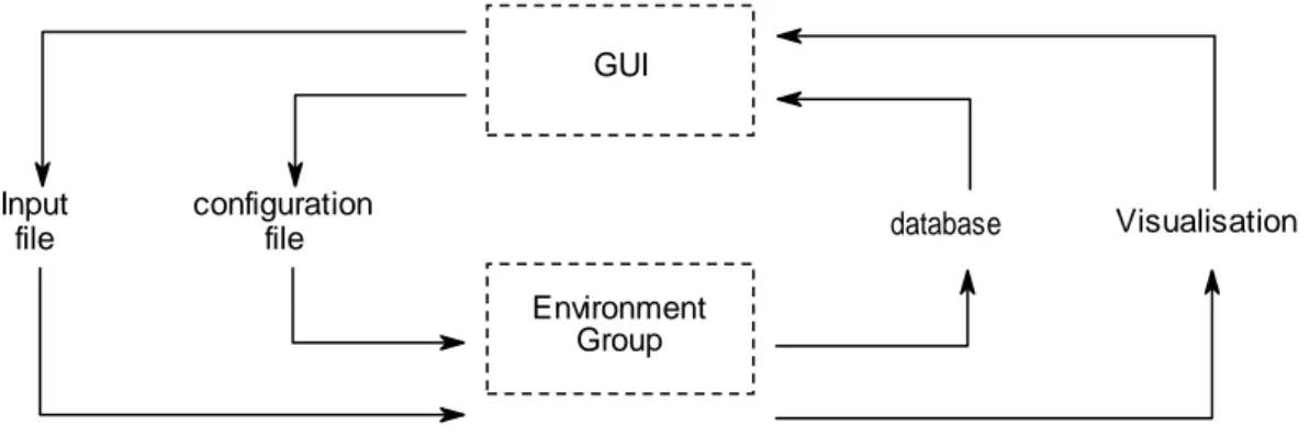
II.3 Schematic connections between warping environment and the GUI. ... 44
II.4 Preview of the GUI. ... 44
II.5 Pressure field along a 2D column of water under gravity ... 46
II.6 Norm L2 of the speed field along a 2D flow of air under gravity... 47
II.7 Graph of the speed in the direction of gravity along the orthogonal direction. 47 II.8 Norm L2 of the speed field along a 2D flow of air under gravity... 48
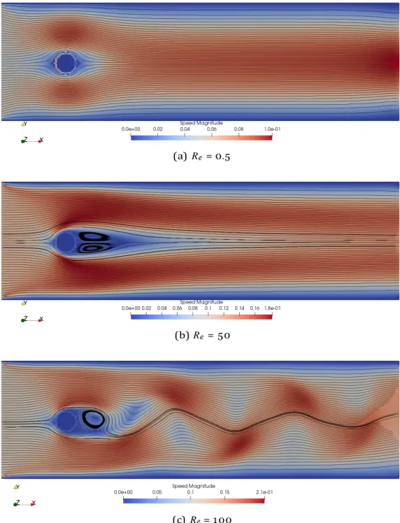
II.9 Graph of the speed in the direction of gravity along the orthogonal direction. 49 II.10... P araView visualization of the streamlines and norm of the speed for Von Kármán vortex street. ... 50
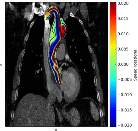
III.1 Illustrative computation of blood flow through an aortic aneurysm from medical image. ... 55
III.2 Schematic of the probability of streaming. ... 57
III.3 Result of segmentation with a LBM anisotropic diffusion reaction [Wan14]. . 58
III.4 Morphological dilation in greyscale using the LBM applied to Lena’s image. 61 III.5 Morphological erosion in greyscale using the LBM applied to Lena’s image. 62 III.6 Use of mathematical morphology in LBM to simulate bone growth from images. ... 63
III.7 Schematic representing the order to use the different LBM layers ... 64
III.8 Result of the thrombus segmentation with a LBM... 65
III.9 Computed velocity of the blood flow inside the aneurysm and its parent vessel 65 III.10Schematic of the thrombosis reaction system ... 66
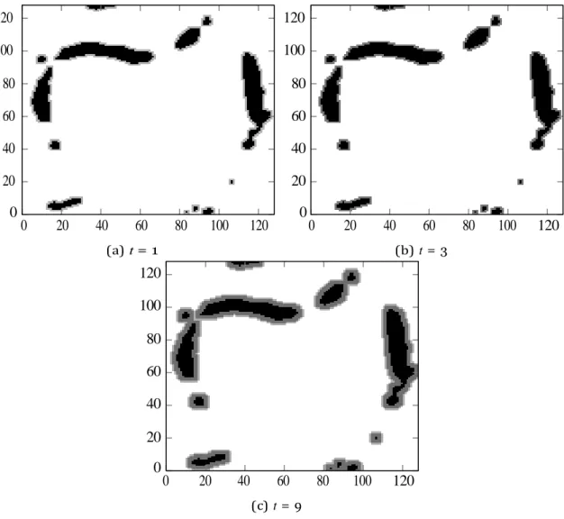
III.11Numerical simulation of the thrombosis growing layer by layer ... 66
III.12Representation of the onionskin structure of the giant aneurysm... 67
IV.1 Organization of the main concepts composing the LBM... 71
IV.2 Schematic of a 1D spring compressed test case and the image associated. . . 80
IV.3 Displacement and density in function of space at the compression steady stage. ... 80
IV.4 Displacement and density in function of space at the decompression steady stage. ...81
IV.5 Schematic of 2D pure shear test case and the image associated...82
IV.6 Displacement colour map and graph of a pure shear stress simulation...82
V.1 Sequence of main concepts composing the LBM ...89
V.2 Displacement in lattice units along the 1D spring at different time step. . . 90
V.3 Speed in lattice units along the 1D spring at different time step. ...90
V.4 Schematic differences between surface and volume forces in LBM ... 91
V.5 Displacement and divergence of the stress in lattice units along the 1D spring at 15 time step...92
V.6 Displacement and divergence of the stress in lattice units along the 1D spring at 150 time step. ...93
V.7 Norm of a shear displacement ant speed at 250 time steps. ...94
V.8 A shear displacement at 2300 time step. ... 95
V.9 Norm of a shear displacement and speed at 2525 time step...95
V.10 A shear displacement at 2650 time step. ... 95
V.11 Schematic of the local compression simulation and its associate image. ...96
V.12 Norm of the displacement and the speed in a 2D-shell locally compressed after 75 time step. ...97
V.13 Norm of the displacement and the speed in a 2D-shell locally compressed after 1555 time step...97
V.14 A displacement at 3000 time step... 98
V.15 A displacement at 7800 time step... 98
V.16 A displacement at 7890 time step... 98
A.1 Schematic of a road with changing of speed limit and number of lane. . . . . 110
A.2 Schematic of an asymmetric D1Q6 network. . . 111
A.3 Schematic of a ring road. . . 114
A.4 Fundamental diagram of some macroscopic models. . . 115
A.5 Flow-density relationship for different relaxation time. . . . 115
A.6 Schematic of merging roads. . . . 116
A.7 Modelling of road merging in free-fl w traffic conditions. . . . 116
A.8 Modelling of road merging in congested-flow traffic conditions. . . . . . . . . 117
A.9 Schematic of a road with number of lane change. . . . 117
A.10 Density for reduction of lanes in free-flow conditions. . . . 118
A.11 Density for a reduction of lanes in congested-fl w traffic conditions. . . 118
A.12 Schematic of a road with a change of speed limit. . . . 119
A.13 Modelling of a road containing a reduction of speed restriction under free- flow traffic conditions. . . . . 119
Romain Noël
A.14 Modelling of a road containing a reduction of speed restriction under congested- flow traffic conditions. ... 120 A.15 Fundamental diagram: flow-density relationship for different lorry concen-
tration. ... 121
List of Tables
I.1 Values of the weight and roots of the usual Gauss-Hermite quadratures. . 27 II.1 Parameters taken for the hydrostatic pressure simulation... 45 II.2 Parameters taken for the Poiseuille flow under gravity simulation. ... 46 II.3 Parameters taken for the Von Kármán vortex street different regimes. . . 51 III.1 Parameters taken for the anisotropic diffusion reaction for segmentation. . . 58Preface
This document is fulfi ment to the grade of Philosophiae Doctor in science. It relate s the research works done between May 2016 and May 2019. In order to help the readi ng, the symbols and notations adopted in this document are listed below.Abbreviations
ASCII American Standard Code for Information Interchange BE Boltzmann Equation
BGK Bhatnagar, Gross and Krook CFD Computational Fluid Dynamics CPU Central Processing Unit
DICOM Digital Imaging and Communications in Medicine FDM Finite Difference Method
FEM Finite Element Method FORTRAN FORmula TRANslator
FPD Fundamental Principe of the Dynamics FVM Finite Volume Method
GAC Geodesic Active Contours GIF Graphics Interchange Format GNU GNU’s Not Unix
GOEDF Generalized Out-Equilibrium Distribution Function GPU Graphical Processing Unit
GUI Graphical User Interface
LBE Lattice Boltzmann Equation
LBGKE Lattice Boltzmann-BGK Equation LBM Lattice Boltzmann Method
LGCA Lattice Gas Cellular Automata MGF Moment-Generating Function MM Mathematical Morphology MPM Material Point Method MRT Multiple Relaxation Time NSE Navier-Stokes Equations NSF Navier-Stokes-Fourier OpenACC Open ACCelerators PDE Partial Differential Equations PGI Portland Group Incorporated QE Quasi-Equilibrium
REV Representative Elementary Volume SPH Smoothed Particle Hydrodynamics VTK Visualization ToolKit
WENO Weighted Essentially Non-Oscillating WSS Wall Shear Stress
XML eXtensible Markup Language
Mathematical conventions
nabla vector ∇ gradient operator ∇ (x) divergent operator ∇ · (x) curl operator ∇ ∧ (x) p-norm lxlpexplicit scalar product (x|y) dyadic product x ⊗ y full contraction x:y
convolution product x y
topological closure x
real set R
Nomenclature
Symbol Description Unit
Distributions
Gi propagation probability ∅
SN skew multivariate normal distribution ∅
f density distribution function over velocity space kg.m−D − 1.s f� generalised out-equilibrium distribution function kg.m−D − 1.s f (0) equilibrium distribution given by the Maxwell-
Boltzmann distribution
kg.m−D − 1.s
f∗ quasi-equilibrium density distribution function kg.m−D − 1.s f�i discretized velocity density distribution function for
the numerical scheme
kg.m−D − 1.s
fN statistical distributions of a N elements system m−D − 1.s
f N truncated density distribution kg.m−D − 1.s fˇ particles distribution function over velocity space m−D − 1.s gi forcing term projected over the velocity space kg.m−D − 1.s
Matrix Variables
B left Green-Cauchy strain tensor ∅
I identity square matrix D × D ∅
MM matrix transformation from distribution space to mo-
ments space
SM diagonal matrix containing the (multiple) relaxation
time of each moments
Λ positive definite matrix that be used to construct a Mahalanobis distance
s−1
s−1
∅
Π viscous stress tensor kg.m.s−1
o linearised strain tensor ∅
λ diagonal standard deviation matrix ∅
o left Cauchy stress tensor kg.m.s−2
I[·]
Operators
integral operator of a given quantity over the velocity space
Pn permutation cyclic index permutation with n different
terms
⊕ morphological dilation
8 morphological erosion Ω(., .) collision-interaction operator
δx Dirac distribution centred on x
Symbol Description Unit
D physical space dimension ∅
Eint
Eint
internal energy of a system internal energy
J kg.m2.s−2
Ek kinematic energy kg.m2.s−2
Etot total energy kg.m2.s−2
Eθ thermal energy kg.m2.s−2
H Gibbs-Boltzmann entropy J.K−1
HN
I
Hamiltonian of the system image function of RD in R
J ∅
MG moment generating function ∅
N number of element in the statistical system ∅ N
Pc
troncature order over the Hilbert basis power of the contact forces
∅ J.s−1
Pg external volume force power J.s−1
Pk kinetic power J.s−1
Q S
thermal energy of a system entropy of a system
J J.K−1
Sf structuring element function, going from RD into ∅
R and such as {x ∈ RD | Sf (x) /= {∞} ∪ {−∞}
1 is bounded
Sm mass source term kg.s−1
T segmentation threshold ∅
V volume of a system mD
VLJ Lennard-Jones interatomic interaction potential J
W work of the external forces not used to generate move- J ment
a parameter of threshold reaction ∅
cs celerity of the sound m.s−1
fi
m
discretized density distribution algebraic precision of the quadrature
kg.m−D − 1.s
∅
mT overall mass of an object in Lagrangian description kg
mp p mass of particles pressure scalar kg kg.m.s−1 q r
number of discretized speed used in the lattice radiation ∅ W.m−D ra interatomic distance m rm s
interatomic distance at absolute zero temperature entropy
m J.K−1
sG variance of the Gaussian measure ∅
t time s
w Gauss measure ∅
Symbol Description Unit
∂V surface delimiting a system mD − 1
∆x increment of space m
∆t increment of time s
Φ sigmoid function based on the error function and used ∅ in the sknew multivariate distribution
εLJ depth coeffi t of the Lennard-Jones interatomic J energy sink θ absolute temperature K κ thermal conductivity mD − 1.s−1 ν cinematic viscosity mD − 1.s−1 ρ mass density kg.m−D ω relaxation frequency s−1 E perturbation order ∅ Tensor Variables
Hn n order Hermite polynomial ∅
Mi i-th moment generated ∅
ak density distribution coordinate in the Hermite poly- ∅
nomial basis
mk k-th moment of the distribution f variable
Variables
A any extensible physical quantity variable
ψ collision invariant variable
Vector Variables
C torque field kg.m.s−2
F macroscopic force acting on an object kg.m.s−2
L angular momentum of an object kg.m.s−1
M torque exerted on an object kg.m.s−2
V centre of gravity speed vitesse of a physical system in Lagrangian description
m.s−1
c microscopic velocity in the v frame m.s−1
g mass force field m.s−2
p generalized coordinates m dx(D) volume measure mD dx(D−1) surface measure mD − 1 q generalized momentum m.s−1 qθ heat flux W.m−D + 1 u displacement field m v x
macroscopic speed field
coordinate Eulerian vector field
m.s−1
Symbol Description Unit
α vector that drive the skewness of the skew multivariate ∅ normal distribution
δ standardised skew vector ∅
µ mean value of a normal distribution ∅
ξ microscopic velocity of particles m.s−1
ξi discretized particles velocity m.s−1
General introduction
Context & Generalities
A Danish proverb, mixed by physicist Niels Bohr and other authors, explains with simplic- ity and pleonasm the idea that “forecasting is always difficult, especially when it concerns
the future”. That is where one of the great science benefi stands, trying to understand
surrounding things, allowing to foresee their future evolution.
The present thesis manuscript follows this idea. In fact, in multiple cases it is useful, i f not necessary, to anticipate the behaviour an object or a material is susceptible to adopt. In order to give answers, when the trajectory of an object like a planet is at stake, the shape and the internal actions do not really matter; and so, Isaac Newton’s science resorts to an equations system and fundamental principles of mechanics. The latter enable to link an object movement and the forces it experiences. In simpler words: an action implies a reaction. But when the light is put on the intern actions and behaviours of the said object, it is necessary to use a finer mechanic that has interest in the continuum medium. This mechanic has to link forces or constraints to the deformation of a material containing no discontinuity.
Thus, to be able to describe the material, continuum medium mechanics needs to obtain constitutive laws linked to each individual material. These behaviour laws are the macroscopic reflect (visible by the human eye and quite generally about a millimetre or centimetre magnitude order) of microscopic interactions between elements in the materi al (molecular aggregate of a tens of nanometres magnitude order). If it is possible to see the se laws from an only macroscopic point of view, it is also very useful to tackle them from a microscopic point of view, since it purveys a finer information on the mechanical state of the material.
The complexity of the microscopic point of view stands in the number of elements or particles (as elementary objects of small size) to be taken into account. So, statistical physics and Ludwig Boltzmann approach allow to work with statistical distributions of elements rather than with a large number of elements. One then talks about mesoscopic point of view. This roughly simplifies the problem as it averages the interactions betwe e n the elements. Thereby, the Boltzmann equation allows to describe the evolution of a distribution of particles submitted to certain actions.
Nevertheless, the complexity of realistic situations requires quite often the nume ri cal tool to give an answer or a satisfying prediction. The terms numerical simulation i s the n employed, in order to name the use of a computer program allowing multiple calculations
based on a mathematical processes and models. When only the macroscopic continuous aspects are studied, the numerical processes like finite differences, volumes or elements are commonly used. On the other hand, numerical simulations interested in mesoscopic systems governed by the Boltzmann equation have benefi from using the LBM. The latter method is blooming nowadays.
Numerical simulations for direct problems (id est interested in predicting the final state of a system knowing its initial state and the actions undergoing) are distinguished into two main categories of uses. The first is for design: when designing a new vehicle, it is essential to ensure the good resistance of its mechanical parts composing. The second category is for diagnostic: when working on an old building, it must be verifi that the building can support them. In this second case, the accuracy of the results depends on the quality of the information provided by the sensors making it possible to measure the properties which will then be injected into the numerical simulations. So, to an equivalent model, if the first category has all the information necessary for computations during design (at least theoretically, since they are supposed to be desired), then the resulting variability of it lies in the precision of the machines shaping mechanical parts; the second has the maximum amount of information provided by the sensors and must compensate for the missing information.
The context of numerical simulations for biomechanical diagnostic is really represen- tative of the second category. It is realistic to consider that the sensor system is limited to imaging systems because the direct sampling is avoided at maximum. So, the natural progression to realize numerical simulations for diagnostic is rather expensive in time, skil l s and money, because it requires successively:
1. to obtain images through a suitable acquisition device;
2. to process images so that only relevant information is kept for the rest of the proce- dure;
3. the use of classical continuous methods on meshes involve reconstructing a 3D geo- metric model based on the processed images;
4. build from the geometric model or images a mesh adapted to the computations that will be required;
5. build a mechano-numerical model from the mesh and properties observed or conjec- tured, allowing the numerical simulation of the studied problem.
Each of these steps involves a potential loss of information. Steps 2, 3 and 4 also requi re scientists to make important assumptions and decisions. A remarkable poi nt i s that i n the vast majority, once the computations are made, the results available on the mesh are projected on the screen of the scientist microcomputer. Since this screen is nothing more than an image displayer, it means that the scientist has started from an image take n by an acquisition system to end with an image used for the interpretation and analysis of the results, to be able to predict. Moreover, the definition of the acquisition system is the maximum precision available without inputting a priori knowledge about the image anatomical structures.
The choice of the method for biomechanical simulation and diagnostic from image s, i s a question not to neglect. Each of these steps also requires time and resources: compute r equipment, electricity... Also, the reduction of one or more steps could bring a considerable
Romain Noël
gain to society. This would make the diagnostic more eff e and faster, either for a building that has suffered a strong earthquake or for a diagnostic of a patient requiring surgery.
A solution to remove step 4 is to avoid to work with standard numerical methods, but with meshless methods. Among the most famous, one can cite the Smoothed Particle Hydrodynamics or the Material Point Method which work on macroscopic particles. Their effi and performances have been proved and they allow nowadays to work on all types of continuum medium (solid, liquid and gas), even if they require more computational time. However, unlike mesh methods, they are not well adapted to perform image processing.
The LBM is also a “meshless” method, with the asset of allowing numerical simulation at a mesoscopic scale. This property is mainly due to the fact that, contrary to other meshless methods, it is based on statistical mechanics. In addition, since the beginning of the 2010s, the method has been applied to image processing with bolstering results. This means that with such a method it is possible to free oneself from step 4, and to carry out in step 2 with the same computational method. This simplifies the whole procedure. Furthermore, the LBM is a computational method known for its computational speed. This speed lies in its explicit and local character, which also makes it highly parallelizable. Despite the important attractions of the LBM in terms of simulation for image-based diagnostic, it does not only have advantages. In particular, its mesoscopic nature makes the work on solid materials or high viscosity fluids difficult. Indeed, only few works on the capacity of the LBM have been conducted, and those works mention some locks. Thus, the use of such a method for the diagnostic from image is not something to be taken for granted because it still requires many developments.
Positioning the problem
Numerical simulations for image-based diagnostics is resource-intensive, but is a source of considerable progress for society, considering the increasing importance of images. Si nce , the LBM responds to many criteria that the numerical simulation for image-based diag- nostic requires, the choice of relying on this method is done. This choice is motivate d by the ambition to bring missing elements to the method. So, the objectives of thi s the si s are to reduce the gap between the LBM and the image-based diagnostic. Indeed, se ve ral scientific locks persist to create such practical approach.
Although it is possible to work on images with the LBM, many image processing techniques have never been transposed nor discovered. This makes the LBM a perfectible and improvable tool to implement image processing algorithms. Moreover, the numerical simulation of fluid flows directly from an image represents an unprecedented experiment. The LBM is known to be effi t when working with liquids and gazes. However, when it comes to solid matter, the LBM seems to encounter difficulties and has to be adapted. The desire to be able to study all types of continuum medium means overcoming the challenge of solids for LBM.
Also, this thesis suggests studying the use of the LBM for the simulation of continuum
medium for image-based diagnostics. This subject is a scientific challenge for both the
theory and the applications within its reach. With the objective of making a complete tool for the simulation of diagnostics from images with LBM, this thesis aims to obtai n a complete pipeline from the image to the simulation, using only the LBM as a computati onal tool.
In order to reach this objective, this manuscript is decomposed in several chapters. The first chapter recovers the context and State of the Art around the subject to exhibit the locks and opportunities which it offers. Since the subject aims to push forward the LBM, the second chapter reviews an implementation and the validation of our own numerical tools that serves as the foundation for the improvements to come. The third chapter explains how it is possible to use images directly as input of a LBM simulation. It also evokes the LBM-based image processing works developed for our purpose. Then, the fourth chapter aims to obtain an arbitrary internal stress with the LBM. This is, of course, motivated by the idea to mimic solid behaviour. To finish, the fifth chapter tackle the solid problem through a different angle: via the Vlasov equation. The manuscript ends with some conclusions and perspectives brought by these research works. The interested reader can also find in the first appendix, an additional work about the use of the LBM to address heterogeneous and multi-class traffic questions.
Look up at the stars and not down at your feet. Try to make sense of what you see, and wonder about what makes the universe exist. Be curious.
Stephan Hawking
I
Context and State of the Art
Contents of the chapter
Abstract of the chapter . . . 6 Résumé du chapitre . . . . . . . . 7 I.1 Introduction . . . . . . . . . . . . . . 7 I.2 Continuum mechanics . . . . . . 7 I.2.1 Macroscopic Lagrangian mechanics . . . 7 I.2.2 Eulerian mechanics . . . . . . 8 I.2.3 Closing relations . . . . . . 10 I.2.4 Macroscopic numerical methods for continuum mechanics ... 11 I.2.4.1 Computational Fluid Dynamics... 11 I.2.4.1.a Methods on mesh . . . 11 I.2.4.1.b Meshless methods . . . 12 I.2.4.2 Computational Solid Dynamics...12 I.2.4.2.a Methods on mesh . . . 12 I.2.4.2.b Meshless methods . . . 13 I.2.5 Particles numerical methods . . . 13 I.3 The Boltzmann equation. . . . . . . 15 I.3.1 Billiards game with N balls . . . 15 I.3.2 Statistical moments . . . . . . 15 I.3.3 Macroscopic Passage formula . . . 16 I.3.4 Collision invariant . . . . . . . 16 I.3.5 The Boltzmann H -theorem . . . 17 I.3.6 Equilibrium distribution. . . . . 17 I.3.7 Euler equations . . . . . . . 18 I.3.8 BGK linearization . . . . . . . 18
5
I.3.9 Chapman-Enskog expansion . . . . . . . 18 I.3.10 Study of the first order: the NSF equations . . . 19 I.4 Lattice Boltzmann Method . . . . . . . . . . . 21 I.4.1 Projection on Hermite basis. . . . . . 21 I.4.1.1 Study of the basis ... 21 I.4.1.2 Projection of the passage formula... 22
I.5.1 The origins from the Lattice-Gas Cellular Automata . . . . . . . . 30 I.5.2 The pioneers . . . . . . . 30 I.5.3 Boundary conditions . . . . . . . 30 I.5.4 Forces . . . . . . . . . . . . . . . . . . . . . . . . . . . 31 I.5.5 Multiphase-Multicomponent . . . . . . . . . . . . . . . 31 I.5.6 Multiple Relaxation Time . . . . . . . . . . . . . . . . . . . 32 I.5.7 Entropic . . . . . . . . . . . . . . . . . . . 32 I.5.8 LBM for solids . . . . . . . 33 I.6 Image-based diagnostic . . . . . . . 33 I.6.1 Some notions about image processing . . . . . . . 33 I.6.1.1 Denoising . . . . . . . 34 I.6.1.2 Classifi . . . . . . . . . . . . . . . . . . 34 I.6.1.3 Segmentation . . . . . . . . . . . 34 I.6.1.4 Morphological image processing . . . . . . . . . . . . . 34 I.6.1.5 Image processing with the lattice Boltzmann method . . . . 34 I.6.2 Image-based diagnostic with macroscopic methods . . . . . . . 35 I.7 Emanating questions . . . . . . . . . . . . . . . . . . . . . . 35 I.8 Conclusion of the chapter . . . . . . . . . . 36
Abstract of the chapter
The LBM is an original method which presents some relevant aspects for image-based diagnostic. Since, the method is relatively younger than the conventional methods for continuum mechanics, it requires more developments to be fully applicable to image-based diagnostic. In particular, as it will be emphasized in this chapter, eff in image processing and computational solid dynamics have to be done with the LBM.
With a top-down approach, this chapter starts looking at the macroscopic scale. This allows to differentiate the Lagrangian from the Eulerian point of view. This difference is also felt in the numerical methods evoked after. As a link between the macroscopic and microscopic scale, the Boltzmann equation starts from the particle dynamics to end up with the Navier-Stokes-Fourier equations. The Boltzmann equation can be
I.4.1.3 Truncation order . . . . 23 I.4.2 Gauss-Hermite quadrature . . . 23 I.4.2.1 Optimization . . . . . 23 I.4.2.2 Usual formulations . . . 24 I.4.3 Discretization in space and time . . . 27 I.4.4 Algorithm: Streaming and colliding . . . 29 I.5 The numerical developments of the LBM . . . 29
solved numerically with the LBM. As many numerical methods, the LBM implies multiple numerical aspects and developments briefly summed up here.
Résumé du chapitre
La LBM est une méthode originale qui présente quelques aspects pertinents pour le di- agnostic à partir images. Étant donné que la méthode est relativement plus jeune que les méthodes conventionnelles de la mécanique des milieux continus, elle nécessite pl us de développements pour être pleinement applicable au diagnostic à partir d’images. En particulier, comme il sera souligné dans ce chapitre, des eff en traitement d’i mage s e t en mécanique computationnelle des solide doivent être faits avec la LBM.
Ce chapitre adopte d’une approche partant du macroscopique vers le microscopique, Le premier permet de différencier le point de vue lagrangien de l’eulérien. Cette différence se ressent également dans les méthodes numériques évoquées par la suite. Puis, pour faire le lien entre l’échelle macroscopique et microscopique, l’équation Boltzmann part de la dy- namique des particules pour arriver aux équations Navier-Stokes-Fourier. L’équation Boltzmann peut être résolue numériquement avec la LBM. Comme beaucoup de méth- odes numériques, la LBM implique de multiples aspects numériques et développements qui sont brièvement résumés ici.
I.1 Introduction
To make this manuscript more comprehensible, the main foundations and concepts relate d to the subject are developed in this chapter. It is the opportunity to introduce the equati ons necessary to understand the ideas presented in this thesis.
In order to highlight the reasons and choices around the subject of the lattice Boltz- mann method for numerical simulation of continuum medium aiming image-based diag- nostics, it is necessary to look closer at equations and current progresses in the domain. This chapter comes back on the great physical principles of the macroscopic mechanics. This allows to understand the main numerical methods to solve this mechanics. Then, a brief review of the Boltzmann equation enables to understand the concepts and develop- ments linking this mesoscopic equation with the macroscopic Navier-Stokes-Fourier equations. This link is also very important to evaluate the advantages of the numerical method based on this equation. So, from this equation the construction of the famous lat- tice Boltzmann method can be done. Once this method is introduced, numerical aspects and developments can be detailed, which leads naturally to unsolved questions.
I.2 Continuum mechanics
I.2.1 Macroscopic Lagrangian mechanics
To describe the dynamics of a macroscopic physical system, one must look at all the physical principles governing its evolution. At first look, these principles are:
• conservation of the mass,
• conservation of the quantity of the movement.
The conservation of the mass, also called the Lavoisier-Lomonosov principle named after the scientists having demonstrated it [dLav89], stipulates that during a mechanical
M
dW
or chemical transformation, the mass of the overall system does not vary with time. This result is translated in the following equation:
dmT
dt = Sm = 0 (I.1)
where mT represents the system and Sm is the mass source term.
The Fundamental Principe of the Dynamics (FPD) [New87] of a body assimilated to its centre of mass reads:
dmT V dt = , Fi i=1 (I.2) with Fi the forces applied to the system which the speed of its centre of mass is V . This
equation expresses the idea that a variation of momentum (or mass times the acceleration) is equal to the sum of the external forces stressing the system.
This FPD must be completed with the possibility for the system to start rotating. This leads to the equation of Euler-Newton:
dL = ,
dt i
i=1
(I.3)
where L is the angular momentum and Mi is the torque associated to the i-th force. This
means that the variation of angular momentum (or angular acceleration) is equal to the sum of the external torque experienced by the system.
With these two equations, one can describe the movement of planets. But it is harder to get information about the internal stress of a compressed spring.
In order to start looking at the internal solicitations of a system it is possible to exploit the two thermodynamics principles. The first is interested in the conservation of the total energy of the system, allowing conversion between energies eventually, and reads:
dEint = dQ + dW (I.4)
dt dt dt
with Eint is the internal energy of the system, Q is the thermal energy of the system and
dt is the power worked by external forces not used to generate movement.
The second thermodynami cs principle introduced by Carnot [Car24], translates the irreversibility of the physical phenomenon, which leads to the following equation:
dS
dt ≥ 0 (I.5)
where S is the entropy of the system, characterizing the disorder can only increase.
I.2.2 Eulerian mechanics
The previous principles and equations are expressed with a global and Lagrangian point of view, i.e. by following the material points in space. To obtain a local Eulerian formulation, it is possible to use the Leibniz-Reynolds transport theorem [Rey03] which can be written: d r dt V(t) A dx(D) = r V(t) ∂A dx(D) + ∂t f ∂V(t) ( vb · n A dx(D−1) (I.6)
where A is an extensive physical quantity which is integrated over the volume V, its-se l f depending on the time. The derivative ∂V represents the surface delimiting this volume, vb
using, the Green-Ostrogradsky divergence theorem [Gre28], it is possible to transform the surface integral into a volume integral and so:
f ∂V(t) (v ⊗ A) · n dx(D−1) = r V(t) ∇x · (v ⊗ A) dx(D) (I.7)
The application of the previous theorem allows to write the mass conservation in an Eulerian formulation through the form:
r r ∂ρ mT = r V(t) ρ dx(D) (I.8) r V(t) ∂t dx (D) + V(t) ∇x · (v ⊗ ρ) dx (D) = V(t) Sm dx (D) (I.9)
where ρ is the volume mass density of the medium. As now, all the integration elements are equal, they can be removed. The expression of the mass conversation in its local Eulerian formulation, also called the continuity equation, reads:
∂ρ
∂t + ∇x · (v ⊗ ρ) = Sm = 0 (I.10)
The local Eulerian formulation of the momentum conservation from the FPD can be obtained in the same manner and is called the first undefined equation of (linear) motion of Cauchy [Cau29]: , Fi = mT g (I.11) i ∂ρv ∂t + ∇x · (ρv ⊗ v) = ∇x · (σ) + ρg (I.12)
where σ represents the internal stress modelled by the Cauchy (second order) stress tensor. Writing the equation of Euler-Newton gives rise to the second undefined equation of Cauchy (angular) motion:
,
Mi = C (I.13)
i
∇x ∧ (σ) = C (I.14)
with C the volumetric torque undergone by the material. This latter field is generally equal to zero in the absence of a magnetic field, which implies symmetry of the stress tensor of Cauchy. This assumption will be used throughout all this document and summarized by the equations
∇x ∧ (σ) = 0 ⇐⇒ σT = σ (I.15a)
∂ρv
∂t + ∇x · (ρv ⊗ v) =∇x · (σ) + ρg (I.15b)
The scalar multiplication of the first equation of Cauchy with a virtual velocity (or real velocity) allows to obtain the local formulation of the virtual work principle [Ber25]:
(∂t (ρv)) · v∗ + (∇x · (ρv ⊗ v)) · v∗ − (∇x · σ) · v∗ − ρg · v∗
= (∂t (ρv)) · v∗ + (∇x · (ρv ⊗ v)) · v∗ − ∇x · (σ · v∗) + σ : (∇x · v∗) − ρg · v∗
= Pk − Pc + σ : (∇x · v∗) − Pg = 0
2
2 −
The integral formulation of the last equation allows the writing of the variational formu- lation of the problem. This latter weak form is used to build the Finite Element Method (FEM). In addition, this last equation identifies the term σ : (∇x · v∗) with the worked
power as defined above (see eq. (I.4)). After injecting this equation into the first principl e of thermodynamics one can write the conservation of total energy:
( v2 \ ∂t ρ + Eint 2 + ∇x · (r v2 l ρ + Eint 2 \ v − σ · v + qθ + r + ρg · v = 0 (I.17)
Finally, using the inequality of Clausius-Duhem [CD67], the writing of the second principle of thermodynamics in local Eulerian formulation gives:
r
∂t (ρs) + ∇x · (ρsv) ≥ θ − ∇x ·
( qθ
θ (I.18)
where r is the thermal radiation and qθ is the heat flux, s is the specifi entropy and θ is
the temperature.
In summary, the evolution of the state of matter is translated by that of the macro- scopic variables ρ, v, σ, θ, id est in 3 dimensions of 14 independent scalar variables or more generally in D-dimension of D2 + D + 2 independent variables. However, the available equations are 1 + (D + D2−D ) + 1 + 1, that is:
• mass conservation (see eq. (I.10)),
• undefined equations of motion (see eq. (I.15)), • first principle of thermodynamics (see eq. (I.17)), • second principle of thermodynamics (see eq. (I.18)).
I.2.3 Closing relations
It is then necessary to have recourse to D2+D 1 supplementary equations to describe the evolution of matter, these are the constitutive laws describing the links that may exist between stress, density, velocity and temperature.
Classic examples of behavioural relationships are for a Newtonian viscous fluid, the stress is linked to the gradient of speed by the following Stokes linear stress constitutive equation 1 σ = ν 2 ( ∇xv + ∇xvT ) . (I.19) When combined with the Fourier law for heat conduction, given by
qθ = κ∇x (θ) (I.20)
one would obtain the famous system:
∂t (ρ) + ∇x · (ρv) = 0 (I.21a)
∂t (ρv) + ∇x · (ρv ⊗ v + p − ν∇x v) = 0 (I.21b)
∂t (Etot) + ∇x · (Etotv + p · v + κ∇x θ) = 0 (I.21c)
with ν the cinematic viscosity and κ the thermal conductivity of the fluid. The system is called the Navier-Stokes-Fourier equations [NSF22].
Another classic example is homogeneous isotropic linear elastic solids, where the rela- tion eq. (I.19) on the facing page is replaced by the Hooke law
σ = C : ε = GJ−5/3
(
Tr (B) \
B − 3 I + K (J − 1) I (I.22)
dx
∂t (u(X, t)) = v F = I + ∇X (u) = dX (I.23)
B = F FT ≈ I + 2ε J = /det (B) (I.24)
χ (x, t) = X = x − u(X, t) ∇x (χ) = dX = F−
dx ∂t (χ) + v∇x (χ) = 0 (I.25) where G and K are respectively the bulk and shear modulus. This leads to the following system
∂t (ρ) + ∇x · (ρv) = 0 (I.26a)
∂t (ρv) + ∇x · (ρv ⊗ v + p − C : ε) = 0 (I.26b)
∂t (Etot) + ∇x · (Etotv + σ · v + κ∇x θ) = 0 (I.26c)
These different behaviours are explained by the different interactions between the molecules that make up matter.
I.2.4 Macroscopic numerical methods for continuum mechanics
The differences of matter behaviour imply differences in the numerical methods employed to simulate them. Here, these methods are divided in two groups, those to simulate fluid and those to simulate solids. Both of these groups are subdivided in conventional methods on mesh and meshless methods.
I.2.4.1 Computational Fluid Dynamics I.2.4.1.a Methods on mesh
It exists several numerical methods to solve the Partial Differential Equations (PDE) related to fluid dynamics. The conventional macroscopic methods to solve these equations require a mesh as a support for the computations. Sorted by order of complexity and precision these methods are:
• Finite Difference Method (FDM): This method uses a Taylor expansion to estimate
the derivatives and solve numerically the PDE. It results in a great advantage of the method, its simplicity. However, when it comes to Computational Fluid Dynamics (CFD) some weaknesses appear. In a general case, it is not a conservative method, some errors are introduced in the mass, momentum and energy conservations. Also, this method has issues with complex geometries [LeV07].
• Finite Volume Method (FVM): This method is intended to solve conservative equa-
tions. It integrates the conservation equation over a small volume and use the di- vergence theorem to evaluates all terms (except sources and sinks) as flux crossing the volume boundary surfaces. So, naturally this method has the advantages to be conservative. It is also easier to work with complex geometries. It is probably the most used method for CFD today. However, it is not straightforward to find an appropriate unstructured mesh compatible with the finite volume method, especially when higher orders are required [VM07].


![Figure III.3 – Result of segmentation with a LBM anisotropic diffusion reaction [Wan14]](https://thumb-eu.123doks.com/thumbv2/123doknet/11624356.304915/89.893.126.724.276.539/figure-iii-result-segmentation-lbm-anisotropic-diffusion-reaction.webp)