This article has been accepted for publication and undergone full peer review but has not been through the copyediting, typesetting, pagination and proofreading process which may lead to differences between this version and the Version of Record. Please cite this article as doi: Ouellet-Proulx Sébastien (Orcid ID: 0000-0003-3816-6340)
Implication of evaporative loss estimation methods in discharge and water temperature modelling in cool temperate climates
Authors:
Sébastien Ouellet-Proulx*, André St-Hilaire* and Marie-Amélie Boucher**
* Canadian Rivers Institute and INRS-ETE; 490 De la Couronne St. Quebec City, Qc, G1K
9A9
** Université de Sherbrooke, department of civil engineering; 2500 Boulevard de l'Université, Sherbrooke, Qc, J1K 2R1
Abstract
Evaporative flux is a key component of hydrological budgets. Water loss through
evapotranspiration reduces volumes available for runoff. The transition from liquid to water vapour on open water surfaces requires heat. Consequently, evaporation act as a cooling mechanism during summer. Both river discharge and water temperature simulations are thus influenced by the methods used to model evaporation. In this paper, the impact of
evapotranspiration estimation methods on simulated discharge is assessed using a semi-distributed model on two Canadian watersheds. The impact of evaporation estimation
methods on water temperature simulations is also evaluated. Finally, the validity of using the same formulation to simulate both of these processes is verified. Five well known
evapotranspiration models and five evaporation models with different wind functions were tested. Results show a large disparity (18-22% of mean annual total evapotranspiration) among the evapotranspiration methods, leading to important differences in simulated discharge (3-25% of observed discharge). Larger differences results from evaporation estimation methods with mean annual divergences of 34-48%. This translates into a
difference in mean summer water temperature of 1-15%. Results also show that the choice of model parameter has less influence than the choice of evapotranspiration method in discharge simulations. However, the parameter values influence thermal simulations in the same order of magnitude as the choice of evaporation estimation method. Overall, the results of this study suggest that evapotranspiration and open water evaporation should be represented separately in a hydrological modelling framework, especially when water temperature simulations are required.
Keywords
Evaporation, evapotranspiration, discharge, water temperature, modelling, CEQUEAU
Data availability statement
The data that support the findings of this study are available on request from the corresponding author. The data are not publicly available due to privacy or ethical restrictions.
1. Introduction
A crucial component of hydrological and water temperature modelling is the mathematical representation of evapotranspiration fluxes. They occur through plant transpiration on vegetated ground and evaporation from open water and bare soil. Open water evaporation is essentially related to vapour pressure deficit between the air above the watercourse and air saturation vapour pressure. Plant transpiration depends on hydrometeorological conditions, soil properties and the characteristics of plant species (Ahrens, 2015). Regardless of the surface of interest, the evaporative processes affect the hydrological system through two keys elements: (i) it reduces the volume of water available for runoff (Jobson, 1980) and (ii) it acts as a cooling mechanism in the summer through latent heat exchange (Caissie et al., 2007).
Estimation models for evapotranspiration are often classified based on their input data (e.g. Oudin et al., 2005). The spectrum of available models includes empirical, temperature-based (e.g. Blaney & Criddle, 1950; Linacre, 1977; Thornthwaite, 1948), radiation-based (e.g. Jensen & Haise, 1963; McGuinness & Bordne, 1972), water budget (e.g. Guitjens, 1982), mass transfer (e.g. Harbeck, 1962) and hybrid methods (Penman, 1948; Monteith, 1965; Priestley & Taylor, 1972).
Comparison of evapotranspiration models for hydrological modelling can be performed by comparing evaporative loss rates to field measurements (Sumner & Jacobs, 2005; Isabelle et
al., 2015). Because of technical considerations and economic constraints, only a small
number of studies include validations with field measurements. Many studies rely exclusively on the subsequent hydrological simulations for indirectly assessing the quality of
instance, Parmele (1972) showed that the cumulative effect of a 20% bias in the estimation of evapotranspiration induces a significant error in the hydrological simulations. Similarly, Oudin et al., (2005) performed an exhaustive comparison of 27 potential evapotranspiration equations on 308 watersheds using four lumped hydrological models. This work highlighted the equivalent efficiency of methods requiring few input data, such as the method of
McGuinness & Bordne (1972), compared to methods with high input data requirements such as the Penman-Monteith method (Monteith, 1965).
During the summer, the main heat loss mechanisms of a river are evaporative (latent) and convective (sensible) heat fluxes as well as longwave radiation reemission (Webb & Zhang, 1997; Maheu et al., 2014). In some systems, evaporative fluxes can dominate and account for up to nearly 100% of river heat loss during the summer (Hannah et al., 2008). In water temperature modelling, most studies estimate latent heat loss (Chikita et al., 2010; Magnusson et al., 2012) using formulations generally based on a mass transfer equation (Harbeck, 1962). Mass transfer models calculate the difference between the actual and saturation water vapour pressure of the air above the river, weighted by a wind function. When precise evaporation measurements are available, a site specific wind function can be adjusted. However, in situ river evaporation data are often difficult to acquire, and modellers commonly have to rely on readily available wind functions to estimate river evaporative fluxes (e.g. Hannah et al., 2004; Leach & Moore, 2010).
To the best of our knowledge, very few publications about river evaporation estimation rely on direct measurements to validate estimation methods. Among them, Benner, (1999) measured hourly evaporation above 1.0 mm/h on the John day River (Oregon, USA).
Creek (British Columbia, Canada) with an hourly average of 0.03 mm/h. No daily value was reported. Maheu et al., (2014) measured a maximum daily evaporation of 6.8 mm in the Little-Southwest Miramichi River (forested watershed in New Brunswick, Canada) and a maximum daily evaporation of 2.8 mm in Catamaran Brook (third order tributary), with mean daily evaporation values of 3.0 mm and 1.0 mm, respectively.
Rosenberry et al., (2007) compared 14 evaporation estimation methods to the Bowen-ratio energy-budget method for a small lake (0.15 km2) in a mountainous area in northeastern USA. They found the best performances using combination methods: Priestley & Taylor (1972), deBruin & Keijman (1979), and Penman (1948). They reported mean daily
evaporation values (averaged for a specific month) ranging between 0.69-3.43 mm (May to November). Spring & Schaefer (1974) measured maximum daily evaporation of 6.22 mm on Babine Lake (British Columbia, Canada) with a mean value of 1.83 mm during the open water season of 1973.
Many models use a single equation to estimate both evapotranspiration and evaporation (Xu & Singh, 2000). For instance, Winter et al. (1995) compared 11 equations to estimate monthly evaporation on Williams Lake in Minnesota (USA). Among the 11 formulations they tested, only one was originally developed to model open water evaporation. Similarly, many hydrological models (e.g. SWAT, CEQUEAU, HYDROTEL, GR4J, and
TOPMODEL) do not distinguish water loss through open water or bare soil evaporation and evapotranspiration. Since these formulations are sometimes employed without prior
investigation, it is reasonable to wonder whether or not a unique equation is suitable to estimate both evapotranspiration and open water evaporation. This question becomes even more relevant when the same formulation is further used for the estimation of latent heat loss
at the water surface in a water temperature modelling framework. The following study is based on the underlying hypothesis that the two processes should be modelled separately using different formulations. Given its impact on water cooling, accurate modelling of evaporative losses is crucial in the context of water release management for dam operators who have to maintain cool water temperatures downstream of dams for fish habitat.
The goal of the present study is to quantify the impact of choosing a particular evaporation or evapotranspiration estimation method on subsequent hydrological and thermal simulations. More specifically, the objectives are: 1) to evaluate the impact of different evapotranspiration estimation methods on discharge simulations in a semi-distributed model; 2) to assess the impact of the implementation of selected evaporation estimation methods on water
temperature simulations; 3) and finally to evaluate the possible limitations of using the same method to estimate both evapotranspiration and open water evaporation for discharge and water temperature modelling.
2. Methodology
2.1. CEQUEAU hydrological and thermal model
Throughout this study, the CEQUEAU hydrological and water temperature model provides a general modelling framework to implement and compare different equations to model evapotranspiration. Different mass transfer equations for open water evaporation are also compared.
The hydrological component of CEQUEAU is a semi-distributed rainfall-runoff model that uses total precipitation and air temperature as inputs to simulate discharge. This rainfall-runoff model is composed of a production function that distributes water vertically and a
transfer function that routes it downstream. This routing is performed on a predefined grid with cells of equal area. The production function considers the total precipitation that falls on the watershed and distributes it into different conceptual reservoirs, with proportions deduced based on information about land use. Possible reservoirs are: lakes and marshes, upper soil, lower soil and rivers. The two soil reservoirs can store and release volumes of water for runoff, depending on the meteorological conditions and on the values of soil-related parameters. Water is also depleted from the soil reservoirs by evapotranspiration. In open water reservoirs (lakes, marshes and rivers), water is lost through evaporation only. Both evapotranspiration and evaporation are estimated using the Thornthwaite (1948) equation.
Once discharge is simulated, the thermal module of CEQUEAU evaluates the heat budget on each grid cell by summing the advective heat fluxes with the various thermal energy fluxes at the air-water interface, according to Equation (1):
tot s IR e c adv
H H H H H H (1)
Where Hadvrepresents the energy exchanged by advective fluxes, Hs is the net solar radiation, HIRis the net longwave radiation re-emitted by the atmosphere above the water course, Hcis the sensible (convective) heat flux and Heis the evaporative flux. Water temperature is then estimated using the ratio of enthalpy (Htot in MJ) over the volume of
water (V in m3) times the heat capacity of water (C= 4.187 MJ m-3 °C-1):
tot w H T VC (2)
The formulation of the Thornthwaite equation as implemented in the CEQUEAU model is presented in Table 1 (Equation (3)). Parameters XIT and XAA can be estimated using
Equations (4) and (5) where TMi is the mean monthly air temperature (°C) during month i. In
the CEQUEAU formulation, ET is adjusted according to the weighting parameter Hrad, which takes into account the day of the year with maximum solar radiation approximated using Equation (6). The parameter JOEVA, which determines when solar radiation reaches a maximum during the year, should be set to 80 when maximum insolation is observed on June 21st.
The actual evapotranspiration is then estimated according to Equation (3)and the fraction of the grid cell occupied by forested area. In its actual form, the model estimates river
evaporation to be a fixed fraction (80%) of the potential evapotranspiration estimated by the hydrological component (Thornthwaite method; Equation (3)). The latent heat loss is
obtained by multiplying the height of water evaporated (m) with the latent heat of vaporization of water considered constant at 2480 MJ m-3.
Overall, the hydrological component of CEQUEAU has 28 parameters, from which 16 have a physical meaning (snowmelt model, evapotranspiration, water routing, etc.). The other 12 parameters are coefficients to be adjusted to achieve the best possible goodness of fit between observed and simulated discharge. The water temperature model has 12 parameters. Those parameters adjust channel geometry, the importance of each energy fluxes and the timing of freezing/thawing. While the parameters XIT and XAA can be estimated according to the meteorology of the watershed, they can also be manually adjusted to better replicate the observed discharge. In the case of thermal modelling, such adjustments impact the
information in St-Hilaire et al., (2000) and (2015), including a complete list of parameters and a full description of the model.
2.2. Evapotranspiration and evaporation formulations
Two approaches were prioritized in the assessment of the evaporation estimation methods. First, we used alternative methods (summarized in Table 1) to estimate evapotranspiration in the hydrological model without changing the structure of the model (i.e. use
evapotranspiration to estimate latent heat loss). Although such formulations are not physically accurate (open water evaporation and evapotranspiration processes are not the same), they replicate the current structure of the model. This step allows for the evaluation of the impact of using different evapotranspiration formulations on discharge simulations, and associated effects on the subsequent thermal modelling. An ideally adapted method would return realistic evaporation estimates and the best discharge and water temperature
estimations when compared to other methods. Second, we kept the original Thornthwaite evapotranspiration method but implemented a mass transfer method for estimating open water evaporation. Alternate wind functions were tested to evaluate latent heat loss. A set of five equations for estimating evapotranspiration and the same number of wind functions for open water evaporation were selected. Those equations and associated assumptions are described further in section 2.2.1.
The evapotranspiration estimation models were selected to compare different levels of complexity (i.e. number of input data), the availability of those input data and their performance according to the recent hydrological literature.
2.2.1.Evapotranspiration
The method of McGuinness & Bordne (ETM-B; McGuinness & Bordne, 1972) was selected
for its good performance compared to more complex methods in a hydrological modelling study (Oudin et al., 2005) while only requiring air temperature and extra-terrestrial radiation as inputs (Table 1; Equation (7)). This method was first implemented for humid regions (Coshocton, Ohio, U.S.) while most evapotranspiration methods were developed for arid regions.
The Priestley-Taylor equation (ETP-T; Priestley & Taylor, 1972) is a simplified version of
Penman (1948) equation for which the evaporation capacity is replaced by the Priestley-Taylor coefficient ( ). This equation (Table I; Equation (8)) showed good performances to estimate both evapotranspiration (Oudin et al., 2005) and open water evaporation
(Rosenberry et al., 2007The α coefficient corresponds to the slope of the regression between equilibrium evaporation and actual evapotranspiration. Although the initial α value was estimated to be 1.26 (Priestley and Taylor, 1972), a wide range of coefficient values have been applied since. Cristea et al. (2013) compiled a list of 52 different α values from the literature, ranging from 0.6 (Oklahoma; Kustas et al., 1996) to 2.47 (southeast Iran; Daneshkar Arasteh & Tajrishy, 2008).
With a level of complexity somewhat superior to Priestley-Taylor, the Kimberly-Penman equation (ETK-P; Wright, 1982) was also retained for comparison in this study (Table 1;
Equation (9)). This is another modification of the Penman (1948) equation, where the wind function ( ; Table 1; Equation (10)) is modulated according to the day of the year (JD) and
wind speed (u2; m s-1) at 2 m height. This equation is considered as a standard equation by the
performance than the original Penman formulation in the context of lumped conceptual hydrological simulation (Oudin et al., 2005).
The Penman-Monteith equation (ETP-M; Monteith, 1965) is the reference method
recommended by the Food and Agriculture Organization of the United Nations (FAO) for evapotranspiration estimation. Among all the methods selected for this study, it has the highest number of input variables (six). Herein, we used a simplified version (Allen et al., 1998) which excludes stomatal and aerodynamic resistances. It is computed using Equation (11).
Lastly, the Morton complementary relationship areal evaporation model (1983) was retained as a higher complexity method (Table 1; Equation (12)). It connects potential
evapotranspiration (ETP) with a wet environment evapotranspiration rate (ETW) to estimate actual evapotranspiration (ETM). Potential evapotranspiration is estimated using a modified
Penman equation (Table 1; Equation (13)) where wet environment evapotranspiration rate is estimated by Equation (14) and (15). The formulation described in Barr et al. (1997) was retained in this study because it showed good performances under similar climate (British Columbia, Canada).
2.2.2.Evaporation
In addition to the aforementioned evapotranspiration equations, the mass transfer equation was used to estimate river evaporation (Equation 16):
s a
E e e (16)
x
u
(17)
This wind function ( ) includes two coefficients: the intercept ( ) controls the importance of the evaporation resulting from vapour pressure deficit, referred to as free convection, while the slope ( ) controls the importance of forced convection or wind induced convection. Table II presents the five wind functions that are compared in this study.
3. Study sites and data
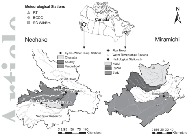
The methodology was applied to two Canadian watersheds: the Nechako River basin (British Columbia) and the Miramichi River basin (New Brunswick). The two watersheds are
spawning grounds for different salmon species and face overheating during the summer. The accurate modelling of their discharge and water temperature is essential for fisheries
management efforts.
3.1. Nechako
The Nechako River is a 45 000 km2 watershed impounded in its upper reaches to create the Nechako reservoir (Figure 1). Its discharge is strongly regulated by the Skins Lake Spillway and flows eastward to the Fraser River. Discharge is recorded at four hydrometric stations on the watershed, namely Skins Lake Spillway, Cheslatta Falls (1 460 km2), the outlet of the Nautley River (6 030 km2) and Vanderhoof (Figure 1; 12 400 km2). Water temperature is recorded at the same location except the Skins Lake Spillway. The spillway is operated by Rio Tinto. During sockeye spawning season, Rio Tinto is required to release sufficient volumes of water to maintain water temperature below 20°C at the confluence of the Nechako and the Stuart rivers (Figure 1). The present paper focuses on the reach of the
station (about 50 km upstream of the confluence with the Stuart River; Figure 1). The model was calibrated to best replicate summer discharge (day 152 to 273) at Vanderhoof but results for all hydrometric stations are shown to allow full appreciation of the model’s capabilities.
Wind speed, atmospheric pressure and relative humidity measurement recorded at Ootsa Lake, Burns Lake and Prince George by Environment and Climate Change Canada (ECCC) were used as model inputs. Precipitation and air temperature measurements from Rio Tinto (RT) and British Columbia Wildfire (BC Wildfire) meteorological stations were also used. Mean annual precipitation of 417 mm (37% as snow) was measured at Ootsa Lake
meteorological station (19812010) with mean daily air temperatures ranging between -11.8°C (January) and 19.8°C (August) and an overall mean value of 3.2°C.
3.2. Miramichi
The Miramichi watershed has a drainage area of 12 000 km2 and has a natural hydrological regime. Water temperature data on the Miramichi watershed were extracted from the RivTemp database (http://rivtemp.ca) for the Southwest Miramichi (SWM; Figure 1) at Wades Lodges, the Little Southwest Miramichi (LSWM; Figure 1) at Oxbow, Northwest Miramichi (NWM; Figure 1) at Call Pool and at Catamaran Brook (CAT; Figure 1).
Discharge data were retrieved from the Water Survey of Canada database on the Southwest branch at Blackville (5 050 km2), on the Little Southwest branch at Lyttleton (1340 km2), on the Northwest branch at Trout Brook (948 km2) and on Catamaran Brook at Repap Road Bridge (28.7 km2). As performed on the Nechako watershed, the model was calibrated to best replicate summer discharge (day 152 to 273) at one site, namely the Southwest Miramichi, but results for all hydrometric stations are presented. Mean annual precipitation of 1072 mm (27% as snow) was measured at the Miramichi A meteorological station with mean daily air
temperatures ranging between -16.6°C (January) and 25.2°C (July) and an overall mean value of 4.6°C.
Benyahya et al. (2010) assessed the difference between observations recorded at a remote meteorological station and observations recorded above the river on the Miramichi watershed (New Brunswick). They found that on the Little Southwest Miramichi River (≈ 80 m width), wind speed measured above the river during the summer was 32.2% of the wind speed recorded at the remote meteorological station, on average. Air temperature, relative humidity and solar radiation were somewhat higher (respectively 103%, 106% and 101%) above the River compared to the meteorological station. Consequently, these corrections were applied to the meteorological observations used in this study.
3.3. Evaporation/Evapotranspiration validation data
Brown et al. (2014) installed two eddy covariance systems in northern British Columbia between 2007 and 2010 at two sites respectively located 100 km (Crooked River) and 160 km (Kennedy Siding) north of Prince George. Average daily evapotranspiration ranged between 1.36 mm (2010) and 1.54 mm (2008) at Crooked River and between 1.12 mm (2007) and 1.21 mm (2009) at Kennedy Siding during the growing season. For the same period, maximum daily evapotranspiration was respectively 3 mm day-1 and 2.5 mm day-1.
In eastern Canada, Malloy & Price (2014) obtained mean daily evapotranspiration of 2.6 mm (2008) and 3.3 mm (2009) in the Bic region (Quebec) during the months of June and July. These values were derived from estimations using Priestley-Taylor (1972) method with an value adjusted using data from five lysimeters. Xing et al. (2008) measured a mean daily evapotranspiration of 1.45 mm and a maximum evapotranspiration of 2.5 mm in the Fredericton region (New Brunswick) from May to October (2004-2007).
Eddy covariance data were also retrieved from the FluxNet database (http://fluxnet.ornl.gov). Latent heat fluxes from the Nashwaak Lake station (2003-2005; Figure 1) were used to calculate evapotranspiration. These evapotranspiration values were used for comparison on the Miramichi watershed.
Brown et al. (2014) calculated coefficients (Equation (10)) of 0.51 and 0.53 using micrometeorological tower data from two sites located close the Nechako watershed (100 km). For the Miramichi watershed, coefficients were calculated based on the
evapotranspiration values derived from the eddy covariance data.
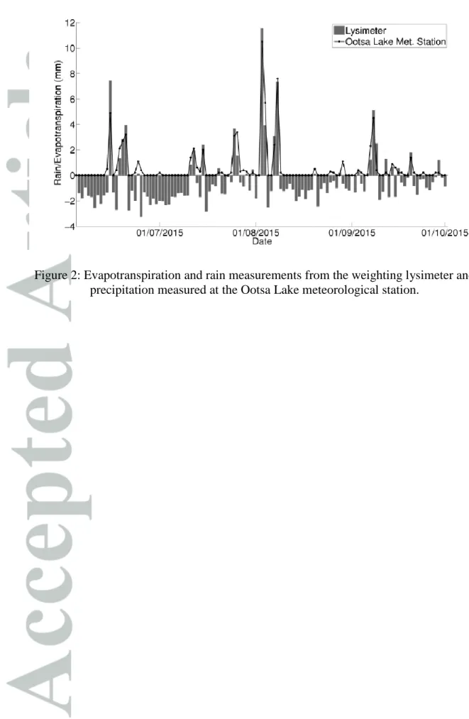
A weighing lysimeter was also installed at about 400 m southeast of the Ootsa Lake/Skins Lake meteorological station (Environment and Climate Change Canada station # 1085836) during summer 2015. The lysimeter was made of a 60 cm soil column constrained in a 12” radius PVC pipe sealed at the bottom. The soil column was placed on a platform scale (PL-100 - UMS) connected to a data logger (CR(PL-1000). The platform scale has a 14 g precision which translates into 0.20 mm of water. Measurements were recorded every 15 minutes between June 4th and October 1rst 2015. Negative differences in weight would indicate evapotranspiration while a positive difference would indicate rainfall. The lysimeter was installed approximately 350 m from the Ootsa Lake meteorological station. Figure 2 presents data recorded using the weighting lysimeter installed on the Nechako watershed between June 4th and October 1st 2015. A maximum evapotranspiration of 3.23 mm was measured with a mean value of 1.33 mm. The total daily precipitation was plotted over the lysimeter data to validate that positive weight variations accurately represent the variation in water content associated with rainfall.
3.4. Model calibration and parameter uncertainty
Both the hydrological and the thermal modules were recalibrated when either the
evapotranspiration or the evaporation method was changed using a split sample method. For the two watersheds, the calibration period is 2001 to 2006 and the validation period is 2007 to 2010. The hydrological component has 28 parameters and the thermal component has 12 parameters. All parameters were optimized using the covariance matrix adaptation evolution strategy (CMA-ES; Hansen & Ostermeier, 1996) with 1500 iterations.
For the hydrological component, the objective function was the maximisation of the Kling-Gupta Efficiency coefficient (KGE) computed for simulated discharge compared to observations. The KGE is a metric proposed by Gupta et al. (2009) that accounts
simultaneously for accurate simulation of the mean discharge, the associated variance and the correlation between simulated and observed discharge. The KGE also puts less emphasis on high discharge values compared to the widely used Nash-Sutcliffe Coefficient (NSE; Nash & Sutcliffe, 1970).
Because of the strong seasonality in water temperature time series, performance metrics such as the KGE or the NSE always tend to be high for modelled water temperature. Hence, they do not have a high discrimination power and are not as informative for this variable as they are deemed to be for discharge. For this reason, the minimisation of the root mean squared error (RMSE) between simulated and observed temperature was used for optimizing the parameters of the thermal module. The Akaike information criterion was also computed, as implemented by Ahmadi-Nedushan et al. (2007), for evapotranspiration on the Miramichi watershed for years with available data. The AIC takes the goodness of fit and the parsimony of the model, through the number of parameters, into account.
The parameters were optimized for each specific evapotranspiration and evaporation methods tested. To compare the impact of the parameters and the impact of the method on the
resulting simulations, a permutation of all 11 sets of parameters and 11 methods was
performed. Performance variation of a given method according to the set of parameters used as well as the performance variation of a given set of parameters according to the method was assessed.
A Kruskal-Wallis test (Kruskal and Wallis, 1952) was performed to verify if the distribution of evapotranspiration values calculated by the different methods have significantly different median. The alternative hypothesis is that at least one of the ET methods yields median values that are significantly different than the others. This test was used instead of the parametric ANOVA because all simulated evapotranspiration series did not meet the assumption of normality. This was verified first, using the Kolmogorov-Smirnov normality test (Massey, 1951). A Tukey-Kramer (Tukey, 1949) test was performed a posteriori to find which methods were not significantly different.
4. Results
4.1. Evapotranspiration
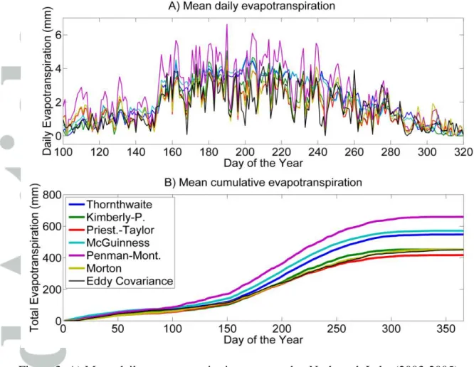
ET measured at Nashwaak Lake using the eddy covariance method were plotted against ET estimated at the same location (selected CEQUEAU grid cell) by the ET methods (Figure 3). Corresponding performance metrics are listed in Table III. In terms of correlation, Kimberly-Penman (r = 70), Priestley-Taylor (r = 72), Kimberly-Penman-Monteith (r = 71) and Morton (r = 73) clearly dominate. All other methods returned r < 0.2. Penman-Monteith returned highly biased ET values (relative bias = 0.46). Priestly-Taylor and Morton returned the lowest biases, with a relative bias of respectively 0.06 and 0.01. According to both metrics, Priestley-Taylor and Morton are the best performing methods to estimate ET. However,
according to AIC values, Priestly-Taylor is considered to be the best method. On average, Morton better replicates total annual ET (Table III; Mean annual bias = 0.89 mm) followed by Kimberly-Penman (Mean annual bias = -7.81 mm). Penman-Monteith has the largest annual bias (Mean annual bias = 207.15 mm).
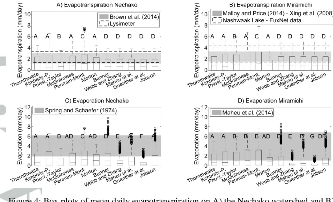
Results of daily ET estimations are presented in Figure 4 (A and B). Grey areas are derived from mean and maximum values found in the literature. The minimum values are not
displayed because they were not mentioned in the cited literature but are expected to be close to zero mm. The middle horizontal line of the boxes represents the annual mean, while the boundaries of the central box represent the 25th and 75th percentiles, the dashed vertical lines are the maximum and minimum values that are not considered as outliers, and the triangles represent outliers.
According to our results, the maximum daily ET ranges between 3.4 mm/day (Priestley-Taylor) and 7.5 mm/day (Penman-Monteith) on the Nechako and between 3.4 mm/day (Morton) and 7.8 mm/day (Penman-Monteith) on the Miramichi. No significant difference is observed when a mass transfer method is used for open water evaporation when computing overall ET on the Miramichi watershed (group A; Figure 4-B) compared to the Thornthwaite equation. Morton’s equation returned values significantly different from all other methods. On the Nechako, all mass transfer methods belong to the same group (group D; Figure 4 - A) but are significantly different from results yielded by the Thornthwaite equation (group A; Figure 4 - A). Kimberly-Penman, McGuinness and Morton methods belong to the same group (group B). When compared to data published by Brown et al., (2014) and our lysimeter data, all methods tested on the Nechako watershed overestimate ET (Figure 4). However, the Priestley-Taylor equation provides results that are less overestimated than all other equations.
On both watersheds, the Kimberly-Penman and the Penman-Monteith equations yielded the highest and the most variable ET values during the summer. It should be noted that those equations are the only ones among our selection that directly include wind speed and air vapour pressure in their formulation. Wind speed, known to be more spatially variable than other variables such as air temperature and relative humidity (Luo et al., 2008), is a potential source of error in the implementation of these methods.
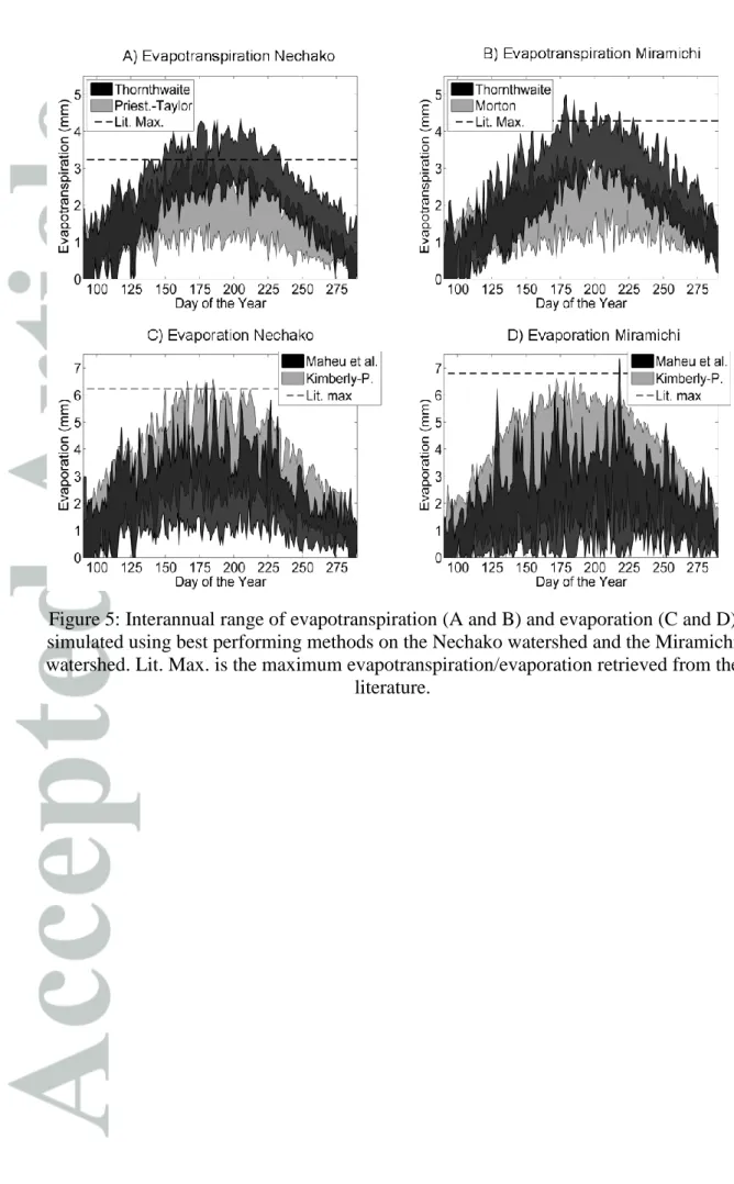
When compared to ET data from the literature and to lysimeter measurements, the most appropriate method on the Nechako watershed is Priestley-Taylor (α = 0.5), followed by Thornthwaite’s equation coupled with a mass transfer equation (regardless of which wind function is used). On the Miramichi, the best performing method is Morton (as shown using the Nashwaak Lake eddy covariance data). When the interannual ranges of estimated values obtained from Morton and Thornthwaite are plotted on the same graph, the lower values simulated by the Morton equation on the Miramichi watershed become obvious (Figure 5 - B). The same pattern is visible on the Nechako for Priestley-Taylor when compared to Thornthwaite’s method Figure 5 – A).
4.2. Evaporation
The maximum daily evaporation ranges between 3.4 mm (Priestley-Taylor; Guenther et al.) and 9.8 mm (Benner) on the Nechako watershed and between 1.96 mm (Guenther et al.) and 8.5 mm (Benner) on the Miramichi watershed. All mass transfer equations returned days with no evaporation on both watersheds. Box plots were also produced for open water evaporation estimations (Figure 4 C and D). The grey area represents the mean and maximum values retrieved from the literature.
More variability among the methods is visible for evaporation (Figure 4 C and D) compared to evapotranspiration (Figure 4 – A and B). On the Nechako watershed, the methods of Thornthwaite, Kimberly-Penman, McGuinness, Morton, Maheu et al. and Jobson belong to the same group (A). McGuinness, Morton and Benner are also not significantly different (D). More diversity among the methods is visible on the Miramichi watershed. Thornthwaite, Kimberly-Penman and Morton are not significantly different (group A). Priestley-Taylor, McGuinness and Penman-Monteith belong to the same group (B), Morton, Benner and Jobson form another group (D) and Maheu et al. and Jobson form the last group (F). The other methods are all significantly different from each other.
Evaporation computed with Penman-Monteith’s and Benner's equations on both watersheds appear overestimated while the Priestley-Taylor, Webb & Zhang and Guenther et al.
equations return large underestimations when compared to data found in the literature (Spring & Schafer, 1974). More overestimation is observed on the Nechako watershed, especially for the Benner wind function, which returned maximum evaporation of 9.8 mm/day. In
comparison, the maximum recorded by Spring & Schafer (1974) was only 6.22 mm/day.
When compared to maximum daily evaporation found in the literature, equations proposed by Maheu et al. and by Kimberly-Penman appear to be the most appropriate. However, when the ranges of values returned by those methods are plotted on the same graph (Figure 5 – B and C), it can be seen that the Kimberly-Penman equation generally estimates higher values than the Maheu et al. equation. On the other hand, the latter is more variable. This leads to large differences in total summer (June to September) evaporation estimations, with mean totals of 391 mm (Kimberly-P.) and 235 mm (Maheu et al.) on the Miramichi watershed and 428 mm (Kimberly-P.) and 260 mm (Maheu et al.) on the Nechako watershed.
4.3. Model calibration
On the Nechako watershed, the KGE ranges between 0.75 and 0.91 in calibration (2001-2006) and between 0.80 and 0.87 in validation (2007-2010; Table IV). For the Thornthwaite, Priestley-Taylor and all mass transfer equations, the relative bias is lower during the
validation period than during the calibration period. On the Miramichi watershed, the KGE ranges between 0.68 and 0.86 in calibration and between 0.64 and 0.80 in validation (Table IV). All relative biases decrease in validation, except for the Penman-Monteith, Maheu et al. and Jobson methods. This decrease can be partly explained by the presence of meteorological stations in the calibration dataset that were not in the validation dataset (Nepisiguit Falls [2001-2006], Doaktown [2001-2009]). This affects the precipitation field and consequently the discharge simulations.
With regards to the water temperature simulations on the Nechako watershed, RMSE values ranging between 0.99°C (Morton) and 1.32°C (Webb & Zhang) are obtained using the calibration dataset and RMSE ranging between 1.31°C (Maheu et al.) and 1.51°C (Webb & Zhang) using the validation dataset (Table V). On the Miramichi, RMSE ranges from 0.98°C (Penman-Monteith) to 1.25°C (McGuinness & Bordne) when the calibration dataset is used and from 1.52°C (Thornthwaite) to 1.82°C (Maheu et al.) in validation.
4.4. Discharge
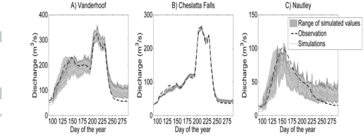
Discharge simulations are shown in Figure 6 (Nechako) and Figure 7 (Miramichi). In Figure 7 – B, it can be seen that the selected ET method has little effect on the simulated discharge at Cheslatta Falls. On average, the difference between the lowest and highest simulated
discharge for the same day is 6.8 m3/s, or 4.9% of the observed discharge at that site. The same value is 28.1 m3/s (55.3 % of observed discharge) at the Nautley station and 51.5 m3/s (25.3% of observed discharge) at Vanderhoof.
KGE values and relative biases calculated for all methods are presented in Table VI. At Cheslatta Falls, all methods used to estimate ET perform similarly well, with a KGE > 0.92. At Vanderhoof, Morton’s method performs best (KGE = 0.95; rel. bias = 0.08), closely followed by the McGuinness & Bordne method (KGE = 0.92; rel. bias = 0.07). On the Nautley watershed, Morton’s equation offers the best results (KGE = 0.75; rel. bias = 0.05) followed by McGuinness & Bordne and Thornthwaite (KGE = 0.74; rel. bias = 0.12).
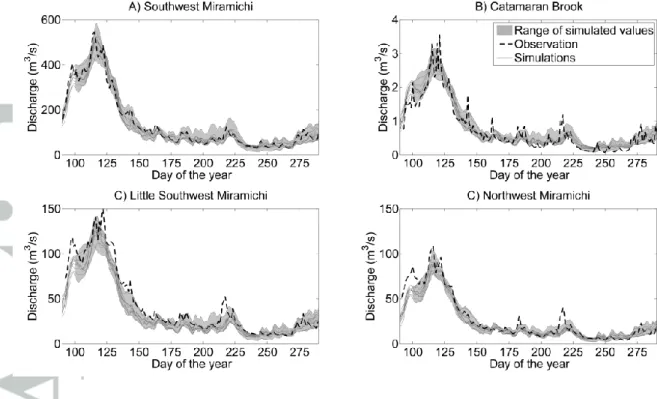
Although the model was calibrated to best replicate discharge on the Southwest branch, it adequately reproduces discharge at all four stations. Underestimation of the spring flood is visible on the Little Southwest Miramichi and some summer peaks are not well reproduced at the three uncalibrated stations. The falling limb of the spring flood simulation is shifted early, toward the winter for all ET estimation methods. According to the KGE, the best performing methods at all four stations are Maheu et al. (KGE = [0.66-0.84]; rel. bias = [0.01-0.11]) and Jobson (KGE = [0.66-0.84]; rel. bias = [0.02-0.11]) closely followed by Penman-Monteith (KGE = [0.65-0.83]; rel. bias = [0.01-0.10]). The poorest results are returned by the McGuinness & Bordne method (KGE = [0.52-0.71]; rel. bias = [0.01-0.23]).
4.5. Water temperature
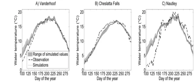
At the Vanderhoof station on the Nechako watershed, all simulated water temperatures stay close to the observations, with some overestimation at the beginning of the summer period (Figure 8). The absolute divergence between the methods ranges from 0.53°C (early August) to 1.34°C (early June). The opposite is visible at the Cheslatta Falls station where water temperature is underestimated between June and September, with absolute differences ranging from 0.12°C (late July) to 1.22°C (mid July). On the Nautley subwatershed, water temperature is strongly overestimated by all methods at the beginning of the summer period
and underestimated at the end of the summer. Better performances are visible from the end of June through the end of August. Differences between daily values of simulated and observed temperatures, ranging between 0.56°C (late September) and 1.41°C (mid July), are induced by the choice of an evaporation estimation method on the Nautley River.
The lowest RMSE (RMSE = 1.28°C; Table VII) at Vanderhoof is obtained when the wind function proposed by Maheu et al. is used. It represents the second best performance at Cheslatta Falls (RMSE = 1.71°C) and the best performance at the Nautley station (RMSE = 2.01°C).
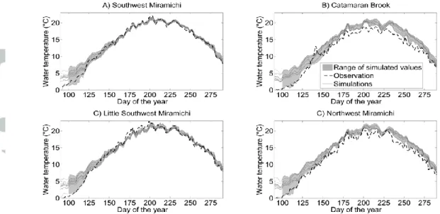
On the Miramichi watershed, a good representation of the seasonal cycle of water temperature is observed on the Southwest Branch during the summer (Figure 9). On
Catamaran Brook and on the Northwest Branch, summer temperature is overestimated (mean bias = 1.14°C) by all evaporation estimation methods while it is underestimated (mean bias = -0.93°C) on the Little Southwest Branch at the beginning of the summer. The differences in water temperatures returned by the different methods go from 0.47°C (early September) to 1.33°C (late June) on the Southwest Branch. This absolute difference goes from 0.48°C (mid-September) to 1.63°C (early August) on the Little Southwest Miramichi. On Catamaran brook, a wider range of values is observed and the differences go from 0.75°C (mid-July) to 3.5°C (early June). Lastly, on the Northwest Branch, the bias on water temperature
simulations ranges from 0.63°C (mid-June) to 2.26°C (late August). The best performances are obtained when using the methods of Kimberly-Penman (Southwest branch;
RMSE = 1.30°C), Benner (Catamaran Brook; RMSE = 2.36°C and Northwest branch; RMSE = 2.11°C) and Priestley-Taylor (Little-Southwest; RMSE = 1.70°C), as shown in Table VII.
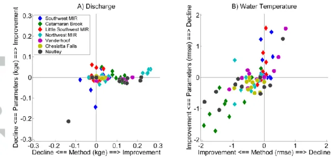
Lastly, Figure 10 presents the performance variations of discharge (A) and water temperature (B) simulations when the different methods are used (x-axis) and when de different sets of parameters are used (y-axis). The difference between the original performance metric when each method is used, with their optimized set of parameters, and their performance when the set of parameters of the best performing method is provided to all methods is plotted of the x-axis. On the y-axis, the difference between the original performance metric and the
performance the best performing method when all sets of parameters to the best performing methods is represented. With regards to the KGE (RMSE), a value located above (below) the horizontal zero line indicates that performances improve when an alternative set of
parameters is used. On the y-axis, a value located on the right (left) side of the zero vertical line indicates an improvement of the KGE (RMSE) when an alternative method is used. Best performing sets of parameters and methods were selected based on results presented in Table VI (discharge) and Table VII (temperature).
Results show that most performance variations in discharge for all Miramichi stations are induced by the selected evapotranspiration method (Figure 10 – A diamonds). The Southwest Miramichi (Figure 10 – A blue diamonds) is more sensible to parameter selection compared to all other stations. On the Nechako, all methods at all three sites are marginally impacted by parameters selection (Figure 10 – A circles), while the selection of ET method influences discharge simulation performances. More scatter can be observed for water temperature, indicating an influence of both the choice of method and the parameters. On the Miramichi watershed, simulation at both the Southwest and the Little Southwest stations are majorly impacted by the parameters (Figure 10 – A, red and blue diamonds). However, simulation performances on Catamaran Brook, and to a lesser extent on the Northwest Miramichi, are influence by both parameter and evaporation method selection (Figure 10 – B, green and
cyan diamonds). On the Nechako, simulation performances at Vanderhoof are mostly impacted by parameter selection (Figure 10 – B purple circles), while method selection dominates for Cheslatta Falls and Nautley stations (Figure 10 – B, grey and yellow circles).
5. Discussion and conclusion
In discharge and water temperature modelling, the choices related to model formulations are key elements to a proper representation of the physical processes, which in turn impact model performance. Evapotranspiration and open water evaporation equations are often
interchanged and used without prior validation. In the absence of field measurements, which is often the case in hydrological studies, it is difficult to validate which method better
represents these variables across a watershed. The results presented in this study offer insights on the consequences associated with modelling choices pertaining to evaporative losses.
5.1. Evapotranspiration and discharge
The estimation of evapotranspiration directly influences discharge simulations. They are discussed together here. In terms of evapotranspiration, the Priestley-Taylor and the Morton methods offer the most realistic estimations on both watersheds when compared to literature and observed data. All the other methods overestimate evapotranspiration on both
watersheds. The methods that overestimate ET the most in this study (Kimberly-Penman and Penman-Monteith) both include wind speed and relative humidity as inputs (Equations (9) and (11)). Data for those two variables can be difficult to acquire, especially if a good spatial resolution is required. The methods of Kimberly-Penman and Penman-Monteith are also the most data intensive formulations, with respectively five and six input variables. Since the methods are used for large watersheds, meteorological inputs are subject to important
uncertainties associated with data interpolation and with the heterogeneity of the area (land use, topography, etc.). On this matter, Droogers and Allens (2002) obtained better
evapotranspiration estimates using a modified Hargreaves method compared to Penman-Monteith. They attribute this result to the inaccuracy of input meteorological data needed for Penman-Monteith.
In terms of discharge, the best performing method at all three validation stations on the Nechako watershed is Morton. However, the method is data intensive as it requires six input variables. On the Miramichi watershed, the Maheu et al. and Jobson equations perform best in terms of simulated discharge (in addition to the Thornthwaite method) at the Southwest and Little Southwest branches stations, while Morton’s equation offers the best performances at the Catamaran Brook and Northwest stations. The Priestley-Taylor and Morton equations better represent evapotranspiration. Nevertheless, no method clearly dominates the others in terms of estimating discharge in this study. A set of methods requiring a small number of input variables (McGuinness & Bordne, Thornthwaite with or without mass transfer, and Priestley-Taylor) returned better discharge simulations compared to more complex methods (e.g. Penman-Monteith) while being easier to implement because of their less extensive data requirements. In previous research, Barr et al. (1997) found good simulation results using Morton’s method. However, no simpler methods were compared. Oudin et al., (2005), showed good hydrological performances using simple methods such as McGuiness and Bordne while concluding that Penman-derived approaches were less advantageous in rainfall-runoff models.
5.2. Evaporation and water temperature
The influence of open water evaporation on water temperature is observed through latent heat loss. To the best of the authors’ knowledge, no such comparative study was previously
performed for both evaporation methods and water temperature modelling. Ouellet et al. (2012), compared the performance of various evaporation methods for subsequent temperature modelling. However, only the best performing method was used for the simulations.
In terms of evaporation, the method of Maheu et al. followed by the method of Penman offer the most realistic estimations on the Nechako watershed, and Kimberly-Penman method, followed by Maheu et al. and McGuinness and Bordne, offer more realistic estimations on the Miramichi watershed. In terms of water temperature simulations for the Nechako watershed, the method of Morton is the best performing method, followed by Maheu et al. For the Miramichi watershed, the method of Kimberly-Penman performs best, followed by the methods of Priestley-Taylor and Thornthwaite. There is thus an apparent adequacy between the ability of these methods to properly estimate evaporation and the performance of the water temperature simulation. This adequacy cannot be extended to evapotranspiration estimation and discharge modelling because the best performing methods were not the same for both processes. These findings support the hypothesis stated in the introduction of this paper, namely that evapotranspiration and evaporation processes should be estimated separately using distinct equations in discharge and water temperature
modelling.
In the present study, the use of a mass transfer equation to estimate open water evaporation does not automatically improve its estimation compared to the use of a method initially
designed to estimate evapotranspiration. An important disparity is observed among the evaporation estimates returned by the mass transfer method with different wind functions. This disparity was observed on the same watershed with different wind functions as well as for the same wind function on different watersheds. For instance, the Webb & Zhang equation, widely used in water temperature modelling (e.g. Leach & Moore, 2010),
underestimates evaporation on both watersheds used in our study. The mass transfer equation is only influenced by two inputs (wind speed and vapour pressure deficit), by the
parameter (free convection) and by the parameter (forced convection). When looking at the distribution of vapour pressure deficit, it can be seen that higher values are estimated on the Miramichi watershed compared to the Nechako watershed. This suggests a greater sensibility of the Miramichi watershed to values, returning low evaporation values if is small. This is coherent with the values obtained with Webb & Zhang equation
( = 0.12 mm/kPa/day) and with Guenther et al. equation ( = 0 mm/kPa/day). In contrast, the Maheu et al. and Jobson equations lead to greater values, respectively 3.09 and 3.01 mm/kPa/day. With regards to wind speed, a larger range of values and a higher frequency of higher wind velocities are observed on the Nechako watershed. Since
multiplies wind speed, it has a greater influence on the Nechako watershed compared to Miramichi. This suggests that the parameters of the wind function of a mass transfer equation should be carefully evaluated in situ before using it to estimate river evaporative fluxes.
5.3. Final selection of method
According to the results obtained in the present study, certain considerations should be well weighed when selecting evapotranspiration and evaporation methods for discharge and water temperature modelling. In this case, the best method to estimate evapotranspiration does not
necessarily results in the best discharge simulation. This inconsistency highlights a dilemma associated with conceptual models in general. Should the adequacy of discharge (or water temperature) simulations take precedence over the good representation of the processes represented by the model? In the context of the implementation of conceptual models, the question is somewhat moot, as the level of conceptualization determines the extent to which processes can be adequately represented. This dilemma can be resolved by increasing model complexity, which is not always possible or desirable because of the operational context and data availability. However, understanding the limits associated with a more conceptual representation of physical processes and quantifying the related uncertainty are of the utmost importance.
The validity of the adjusted parameters should also be considered when evaluating
evapotranspiration estimation methods based on subsequent simulation results. Clark et al. (2015) showed the equivalent and sometimes stronger influence of model parameters compared to processes representation on the modelling uncertainty. In this study, the impact of parameters was found more important in thermal simulations than in hydrological
simulations. In both cases, the influence of the parameters selection was more important at the calibration stations compared to other validation sites on the watershed.
Many hydrological studies go beyond a good reproduction of observed discharge at a specific site and require a realistic representation of the hydrology of a watershed. Climate projection studies over large watersheds (e.g. Morrison et al. 2002) are good examples of such
applications. Thompson et al. (2014) showed that evapotranspiration estimation induces uncertainty in future discharge projections using climate change scenarios. In such a context, an evaporative loss estimation method should be selected for its ability to adequately
represent the evaporative response to changing atmospheric conditions. The question of whether or not the chosen evaporative loss method leads to an ideal simulation of discharge appears secondary in that context. However, results suggest that river evaporation marginally contributes to total water loss though evaporative processes. Efforts should thus first be concentrated on evapotranspiration in studies interested in discharge simulations.
In conclusion, the present study concentrates on various evapotranspiration and open water evaporation estimation methods that were evaluated in a discharge-water temperature modelling cascade. The comparison of five evapotranspiration equations and five mass transfer equations revealed an important uncertainty on both discharge and water temperature carried by the modelling of these processes. Yet, no method clearly outperforms the others for all validation stations. Finally, our results suggest that the method used to estimate evapotranspiration and open water evaporation, especially in a water temperature modelling context, should be established separately and not solely based on the subsequent simulation results. A careful attention should also be given to parameters selection as their uncertainty can dominate over processes uncertainty. Ensemble simulations through multimodule
methods would allow the representation of these uncertainty sources into a modelling process (e.g. Clark et al., 2015).
6. Acknowledgements
This work was funded in part by NSERC and Rio Tinto. The authors wish to thank J. Benckhuysen, B. Larouche and M. Latraverse for their assistance in the realization of this project.
7. References
Ahmadi-Nedushan B, St.-Hilaire A, Ouarda TBMJ, Bilodeau L, Robichaud É, Thiémonge N, Bobée B. 2007. Predicting river water temperatures using stochastic models: Case study of the Moisie River (Québec, Canada). Hydrological Processes 21 (1): 21–34 DOI: 10.1002/hyp.6353
Ahrens CD. 2015. Essentials of meteorology : an invitation to the atmosphere. Stamford, CT Cengage Learning.
Allen RG, Pereira LS, Raes D, Smith M. 1998. Crop evapotranspiration: Guidelines for
computing crop requirements - FAO Irrigation and Drainage Paper No.56. DOI:
10.1016/j.eja.2010.12.001
Allen RG, Walter IA, Elliot RL, Howell TA, Itenfisu D, Jensen ME, Snyder R. 2005. The ASCE standardized reference evapotranspiration equation. Reston, VA.
Andersson L. 1992. Improvements of Runoff Models - What Way to Go? Nordic Hydrology 23 (5): 315–315 DOI: 10.2166/nh.1992.022
Barr AG, Kite GW, Granger R, Smith C. 1997. Evaluating three evapotranspiration methods in the SLURP macroscale hydrological model. Hydrological Processes 11 (13): 1685– 1705 DOI: 10.1002/(SICI)1099-1085(19971030)11:13<1685::AID-HYP599>3.0.CO;2-T
Benner DA. 1999. Evaporative Heat Loss of the Upper Middle Fork of the John Day River, Northeastern Oregon. Oregon State University.
Benyahya L, Caissie D, El-Jabi N, Satish MG. 2010. Comparison of microclimate vs. remote meteorological data and results applied to a water temperature model (Miramichi River, Canada). Journal of Hydrology 380 (3–4): 247–259 DOI: 10.1016/j.jhydrol.2009.10.039 Blaney HF, Criddle WD. 1950. Determining water requirements in irrigated areas from
Agriculture, Soil Conservation Service. Washington, DC.
Brown MG, Black TA, Nesic Z, Foord VN, Spittlehouse DL, Fredeen AL, Bowler R, Grant NJ, Burton PJ, Trofymow J a., et al. 2014. Evapotranspiration and canopy characteristics of two lodgepole pine stands following mountain pine beetle attack. Hydrological
Processes 28 (8): 3326–3340 DOI: 10.1002/hyp.9870
Caissie D, Satish MG, El-Jabi N. 2007. Predicting water temperatures using a deterministic model: Application on Miramichi River catchments (New Brunswick, Canada). Journal
of Hydrology 336: 303–315 DOI: 10.1016/j.jhydrol.2007.01.008
Chikita KA, Kaminaga R, Kudo I, Wada T, Kim Y. 2010. Parameters determining water temperature of a proglacial stream: The Phelan Creek and the Gulkana Glacier, Alaska.
River Research and Applications 26 (8): 995–1004 DOI: 10.1002/rra.1311
Clark MP, Nijssen B, Lundquist JD, Kavetski D, Rupp DE, Woods R a, Freer JE, Gutmann ED, Wood AW, Gochis DJ, et al. 2015. A unified approach for process-based
hydrologic modeling: 2. Model implementation and case studies. Water Resources
Research 51 (4): 1–28 DOI: 10.1002/2015WR017198.A
Cristea NC, Kampf SK, Burges SJ. 2013. Revised Coefficients for Priestley-Taylor and Makkink-Hansen Equations for Estimating Daily Reference Evapotranspiration. Journal
of Hydrologic Engineering 18 (10): 1289–1300 DOI:
10.1061/(ASCE)HE.1943-5584.0000679
Daneshkar Arasteh P, Tajrishy M. 2008. Calibrating Priestley- Taylor model to estimate open water evaporation under regional advection using volume balance method—Case study: Chahnimeh Reservoir, Iran. Journal of Applied Sciences 8: 4097–4104
deBruin HAR, Keijman JQ. 1979. The Priestley-Taylor Evaporation Model Applied to a Large, Shallow Lake in the Netherlands. Journal of Applied Meteorology 18 (7): 898– 903 DOI: 10.1175/1520-0450(1979)018<0898:TPTEMA>2.0.CO;2
Droogers, P, Allen, RG, 2002. Estimating reference evapotranspiration under inaccurate data conditions. Irrigation and Drainage Systems 16: 33–45 doi:10.1023/A:1015508322413 Granger RJ, Gray DM. 1989. Evaporation from natural nonsaturated surfaces. Journal of
Hydrology 111 (1–4): 21–29 DOI: 10.1016/0022-1694(89)90249-7
Guenther SM, Moore RD, Gomi T. 2012. Riparian microclimate and evaporation from a coastal headwater stream, and their response to partial-retention forest harvesting.
Agricultural and Forest Meteorology 164: 1–9 DOI: 10.1016/j.agrformet.2012.05.003
Guitjens JC. 1982. Models of alfalfa yield and evapotranspiration. American Society of Civil
Engineers 108 (IR3): 212–222
Gupta H V., Kling H, Yilmaz KK, Martinez GF. 2009. Decomposition of the mean squared error and NSE performance criteria: Implications for improving hydrological modelling.
Journal of Hydrology 377 (1–2): 80–91 DOI: 10.1016/j.jhydrol.2009.08.003
Hannah DM, Malcolm I a., Soulsby C, Youngson AF. 2004. Heat exchanges and
temperatures within a salmon spawning stream in the Cairngorms, Scotland: Seasonal and sub-seasonal dynamics. River Research and Applications 20 (6): 635–652 DOI: 10.1002/rra.771
Hannah DM, Malcolm IA, Soulsby C, Youngson AF. 2008. A comparison of forest and moorland stream microclimate, heat exchanges and thermal dynamics. Hydrological
Processes 22 (7): 919–940 DOI: 10.1002/hyp.7003
Hansen N, Ostermeier A. 1996. Adapting Arbitrary Normal Mutation Distributions in Evolution Strategies: The Covariance Matrix Adaptation. Evolutionary Computation,
1996., Proceedings of IEEE International Conference on: 312–317 DOI:
10.1109/ICEC.1996.542381
Harbeck GE. 1962. A practical field technique for measuring reservoir evaporation utilizing mass-transfer theory. United States Geological Survey Professional Paper 272–E: 101–
105
Isabelle P-E, Nadeau DF, Rousseau AN, Coursolle C, Margolis H a. 2015. Applicability of the Bulk-Transfer Approach to Estimate Evapotranspiration from Boreal Peatlands.
Journal of Hydrometeorology 16 (4): 1521–1539 DOI: 10.1175/JHM-D-14-0171.1
Jensen ME, Haise HR. 1963. Estimating evapotranspiration from solar radiation. American
Society of Civil Engineers 89 (LR4): 15–41
Jobson HE. 1980. Thermal modeling of flow in the San Diego aqueduct, California, and its relation to evaporation. United States Geological Survey. Professional Paper 1122. US Department of Interior: Washington, DC; 24.
Kruskal WH, Wallis WA. 1952. Use of ranks in one-criterion variance analysis. Journal of
the American Statistical Association 47 (260): 583–621 DOI:
10.1080/01621459.1952.10483441
Kustas WP, Stannard DI, Allwine KJ. 1996. Variability in surface energy flux partitioning during Washita ’92: Resulting effects on Penman-Monteith and Priestley-Taylor parameters. Agricultural and Forest Meteorology 82 (1–4): 171–193 DOI: 10.1016/0168-1923(96)02334-9
Leach JA, Moore RD. 2010. Above-stream microclimate and stream surface energy
exchanges in a wildfire-disturbed riparian zone. Hydrological Processes 24 (17): 2369– 2381 DOI: 10.1002/hyp.7639
Linacre ET. 1977. A simple formula for estimating evaporation rates in various climate, using temperature data alone. Agricultural Meteorology 18: 409–424
Luo W, Taylor MC, Parker SR. 2008. A comparison of spatial interpolation methods to estimate continuous wind speed surfaces using irregularly distributed data from England and Wales. International Journal of Climatology 28 (7): 947–959 DOI: 10.1002/joc Magnusson J, Jonas T, Kirchner JW. 2012. Temperature dynamics of a proglacial stream:
Identifying dominant energy balance components and inferring spatially integrated hydraulic geometry. Water Resources Research 48 (6) DOI: 10.1029/2011WR011378 Maheu A, Caissie D, St-Hilaire A, El-Jabi N. 2014. River evaporation and corresponding heat
fluxes in forested catchments. Hydrological Processes 28 (23): 5725–5738 DOI: 10.1002/hyp.10071
Malloy S, Price JS. 2014. Fen restoration on a bog harvested down to sedge peat: A hydrological assessment. Ecological Engineering 64: 151–160 DOI:
10.1016/j.ecoleng.2013.12.015
McGuinness JL, Bordne EF. 1972. A comparison of lysimeter-derived potential evapotranspiration with computed values. Technical Bulletin 1452, Agricultural Research Service, US Department of Agriculture, Washington, DC.
Monteith JL. 1965. Evaporation and environment. Symposia of the Society for Experimental
Biology 19: 205–234 DOI: 10.1613/jair.301
Morton FI. 1983. Operational estimates of areal evapotranspiration and their significance to the science and practice of hydrology. Journal of Hydrology 66 (1–4): 1–76 DOI: 10.1016/0022-1694(83)90177-4
Nash JE, Sutcliffe J V. 1970. River flow forecasting through conceptual models part I - A discussion of principles. Journal of Hydrology 10 (3): 282–290 DOI: 10.1016/0022-1694(70)90255-6
Oak Ridge National Laboratory Distributed Active Archive Center (ORNL DAAC). 2015. FLUXNET Web Page. Available online [http://fluxnet.ornl.gov] from ORNL DAAC, Oak Ridge, Tennessee, U.S.A. Accessed June 5, 2017.
Ouellet, V, Secretan, Y, St-Hilaire, A, Morin, J, 2014. Water temperature modelling in a controlled environment: Comparative study of heat budget equations. Hydrological Processes 28, 279–292. doi:10.1002/hyp.9571
Oudin L, Michel C, Anctil F. 2005. Which potential evapotranspiration input for a lumped rainfall-runoff model? Journal of Hydrology 303 (1–4): 275–289 DOI:
10.1016/j.jhydrol.2004.08.025
Parmele LH. 1972. Errors in output of hydrologic models due to errors in input potential evapotranspiration. Water Resources Research 8 (2): 348–359 DOI:
10.1029/WR008i002p00348
Penman HL. 1948. Natural Evaporation from Open Water, Bare Soil and Grass. The Royal
Society 193 (1032): 120–145 DOI: 10.1098/rspa.1948.0037
Priestley CHB, Taylor RJ. 1972. On the Assessment of Surface Heat Flux and Evaporation Using Large-Scale Parameters. Monthly Weather Review 100 (2): 81–92 DOI:
10.1175/1520-0493(1972)100<0081:OTAOSH>2.3.CO;2
Rosenberry DO, Winter TC, Buso DC, Likens GE. 2007. Comparison of 15 evaporation methods applied to a small mountain lake in the northeastern USA. Journal of
Hydrology 340 (3–4): 149–166 DOI: 10.1016/j.jhydrol.2007.03.018
Spittlehouse DL. 1989. Estimating evapotranspiration from land surfaces in British Columbia. In Estimation of Areal Evapotranspiration. IAHS Publication; 245–253. Spring K, Schaefer DG. 1974. Mass transfer evaporation estimates for Babine Lake, British
Columbia. Downsview, ON.
St-Hilaire A, Boucher M-A, Chebana F, Ouellet-Proulx S, Zhou Q-X, Larabi S, Dugdale S. 2015. Breathing a new life to an older model: the CEQUEAU tool for flow and water temperature simulations and forecasting. In Canadian Society of Civil Engineering
Conference Paper: L’eau Pour Le Développement Durable : Adaptation Aux Changements Du Climat et de L’environnement. Montreal.
St-Hilaire A, Morin G, El-Jabi N, Caissie D. 2000. Water temperature modelling in a small forested stream: implication of forest canopy and soil temperature. Canadian Journal of
Civil Engineering 27 (6): 1095–1108 DOI: 10.1139/l00-021
Sumner DM, Jacobs JM. 2005. Utility of Penman-Monteith, Priestley-Taylor, reference evapotranspiration, and pan evaporation methods to estimate pasture evapotranspiration.
Journal of Hydrology 308 (1–4): 81–104 DOI: 10.1016/j.jhydrol.2004.10.023
Thompson JR, Green AJ, Kingston DG. 2014. Potential evapotranspiration-related uncertainty in climate change impacts on river flow: An assessment for the Mekong River basin. Journal of Hydrology 510: 259–279 DOI: 10.1016/j.jhydrol.2013.12.010 Thornthwaite CW. 1948. An Approach toward a Rational Classification of Climate.
Geographical Review 38 (1): 55 DOI: 10.2307/210739
Tukey JW. 1949. Comparing individual means in the analysis of variance. Biometrics 5 (2): 99–114 DOI: 10.2307/3001913
Webb BW, Zhang Y. 1997. Spatial and seasonal variability in the components of the river heat budget. Hydrological Processes 11 (1): 79–101 DOI: 10.1002/(SICI)1099-1085(199701)11:1<79::AID-HYP404>3.0.CO;2-N
Winter TC, Rosenberry DO, Sturrock AM. 1995. Evaluation of 11 Equations for Determining Evaporation for a Small Lake in the North Central United States. Water Resources
Research 31 (4): 983–993 DOI: 10.1029/94WR02537
Wright JL. 1982. New Evapotranspiration Crop Coefficients. Proceedings of the American
Society of Civil Engineers, Journal of the Irrigation and Drainage Division 108 (IR2):
57–74
Xing Z, Chow L, Meng FR, Rees HW, Stevens L, Monteith J. 2008. Validating
evapotranspiration equations using bowen ratio in New Brunswick, Maritime, Canada.
Sensors 8 (1): 412–428 DOI: 10.3390/s8010412
Xu C-Y, Singh VP. 2000. Evaluation and generalization of radiation-based methods for calculating evaporation. Hydrological Processes 349 (January 1999): 339–349
Xu CY, Singh VP. 2005. Evaluation of three complementary relationship evapotranspiration models by water balance approach to estimate actual regional evapotranspiration in different climatic regions. Journal of Hydrology 308 (1–4): 105–121 DOI:
Figure 1: Maps of the Nechako and the Miramichi watersheds. On the map for Miramichi, Q stands for discharge, T for water temperature, NWM for Northwest Miramichi, LSWM for
Figure 2: Evapotranspiration and rain measurements from the weighting lysimeter and precipitation measured at the Ootsa Lake meteorological station.
Figure 3: A) Mean daily evapotranspiration measured at Nashwaak Lake (2003-2005) and corresponding estimations and B) Cumulative evaporation and corresponding estimations.
Figure 4: Box plots of mean daily evapotranspiration on A) the Nechako watershed and B) the Miramichi watershed and mean daily river evaporation on C) the Nechako watershed and
D) the Miramichi watershed during the summer (June-September). Methods with matching letters (A-D) do not have significantly different median values according the Kruskal-Wallis
Figure 5: Interannual range of evapotranspiration (A and B) and evaporation (C and D) simulated using best performing methods on the Nechako watershed and the Miramichi watershed. Lit. Max. is the maximum evapotranspiration/evaporation retrieved from the
Figure 6: Discharge simulations on the Nechako watershed at A) Vanderhoof, B) Cheslatta Falls and C) at the outlet of the Nautley River.
Figure 7: Simulated and observed discharge on the A) Southwest Miramichi, B) Catamaran Brook, C) Little Southwest Miramichi and D) Northwest Miramichi.
Figure 8: Water temperature simulations on the Nechako at A) Vanderhoof, B) Cheslatta Falls and C) at the outlet of the Nautley River.
Figure 9: Water temperature simulations on the A) Southwest Miramichi, B) Catamaran Brook, C) Little Southwest Miramichi and D) Northwest Miramichi.
Figure 10: Scatter plots of the differences between the original performance metric and the performance metric when best method is used (x-axis) and the differences between the original performance metric and the performance metric when best set of parameters is used