Empirical Analysis of Imbalance Countering Strategies
in Binary Classification
Mémoire
Jonathan Gingras
Maîtrise en informatique - avec mémoire
Maître ès sciences (M. Sc.)
Empirical Analysis of Imbalance Countering
Strategies in Binary Classification
Mémoire
Jonathan Gingras
Sous la direction de:
Résumé
De nos jours, les algorithmes de classification binaire sont utilisés dans des tâches touchant plusieurs champs d’applications comme les fraudes en-ligne, le dépistage bio-médical ou bien la toxicité en-ligne. Malgré le nombre de données qui est souvent disponible pour ces applications, qui viennent habituellement de source réelles, une particularité y est fréquemment observée: la représentation débalancée des classes. Cette imbalance demeure un problème d’envergure pour les algorithmes de classification, car la vaste majorité d’entre eux ne sont pas conçus avec cette représentation inégale à l’esprit. De plus, dans les paramètres expérimentaux, les données sur lesquelles ils sont appliqués sont souvent bien balancées, à cause de la finalité-même de ces expérimentations.
Dans le présent mémoire, une revue des stratégies et techniques existantes pour contrer l’imbalance binaire est proposée, dans laquelle un point de vue par modification de données ainsi qu’un point de vue par modification algorithmique seront adressés. Le premier sujet des présents travaux consiste en les approches de pré-traitement et leurs effets sur les métriques de classification, dans lequel des expérimentations contrôlées (présentant différents niveaux de débalancement) et des applications d’entreprises sont présentées et analysées. Le second sujet consiste en le paradigme sensible-au-coût appliqué à l’optimisation directe de la métrique de la F-mesure en utilisant un réseau de neurones, dans lequel des expérimentations sur un jeu de données très débalancé sont présentées et discutées, le tout accompagné d’une comparaison avec différents paramètres usuels.
À la lecture du présent document, le lecteur aura une bonne idée des techniques de pré-traitement existantes et ce qu’on peut en retirer d’un point de vue expérimental selon des ensembles de données variés. Également, l’application du paradigme sensible-au-coût par optimisation de la F-mesure donnera un aperçu positif quant au point de vue algorithmique dans un contexte de données très débalancées.
Abstract
Nowadays, binary classification algorithms are used in detection-related tasks touching many fields of application such as online frauds, biomedical screening, or online toxicity. Despite the amount of data that’s usually available for those applications, which habitually comes from real-world data sources, a particularity is frequently observed in it: the imbalanced represen-tation of the classes. This imbalance remains a significant problem for binary classification algorithms, because the vast majority of these algorithms are not designed with this unequal representation in mind. Moreover, in experimental setups, the data on which they are usually applied is more than often well-balanced, because of the very purpose of these experiments. In the current thesis, a review of the existing strategies and techniques to face the binary im-balance problem is proposed in which both a data-modification point of view and a algorithm-modification point of view are addressed. The first subject of this work are data prepocessing approaches and their effects on classification metrics, in which both controlled experimental setups (showing different levels of imbalance), and enterprise data applications are presented and analyzed. The second subject is the cost-sensitive paradigm applied to the direct op-timization of the F-measure metric using a neural network, in which experimentations on a highly imbalanced data set are presented and discussed, as well as comparisons with different common settings.
After reading the current document, the reader will be well aware of the existing preprocessing techniques and what they can be achieve in an experimental context using various data sets. Moreover, the application of the cost-sensitive paradigm by optimization of the F-measure will give positive insight regarding the algorithmic point of view in a context of very imbalanced data.
Contents
Résumé iii
Abstract iv
Contents v
List of Tables vii
List of Figures ix
Thanks xi
Introduction 1
1 Background 3
1.1 Machine Learning Basics . . . 3
1.2 Theoretical Foundations . . . 8
1.3 Learning Methodology . . . 16
1.4 The Class Imbalance Problem . . . 19
2 Data Preprocessing 26 2.1 Undersampling . . . 26
2.2 Undersampling relying on heuristics . . . 28
2.3 Oversampling . . . 29
2.4 Experiments. . . 31
2.5 Industrial Case Study: Two Hat Security. . . 47
3 Cost-Sensitive Learning & Optimization Of The F-measure 54 3.1 Motivation Behind The Cost-Sensitive Paradigm . . . 54
3.2 Theoretical Foundation Of Cost-Sensitive Learning . . . 55
3.3 Optimizing the F-measure . . . 56
3.4 Experiments. . . 59
Conclusion 71
A Resampling Exhaustive Results 73
List of Tables
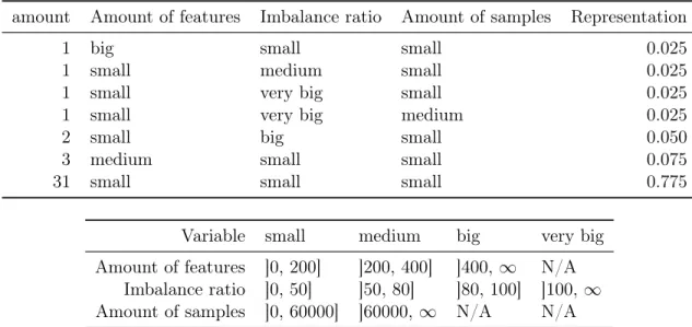
2.1 Representation of variables in group combinations of data sets. . . 34
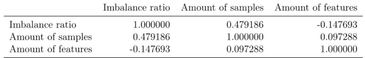
2.2 Correlations between data set variables. . . 35
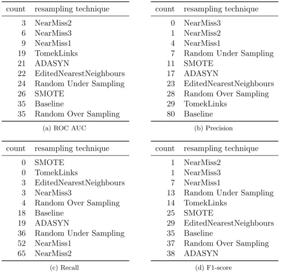
2.3 Count of times each resampling technique was the best considering the 200 combinations learning algorithm - dataset, per metric . . . 37
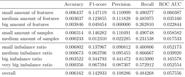
2.4 Maximum improvement per metric (every pair of learning algorithms and resam-pling techniques considered) in terms of groups of data set variables according to table 2.1 . . . 40
2.5 Differences of Accuracy against baseline per algorithm and preprocessing tech-nique. . . 42
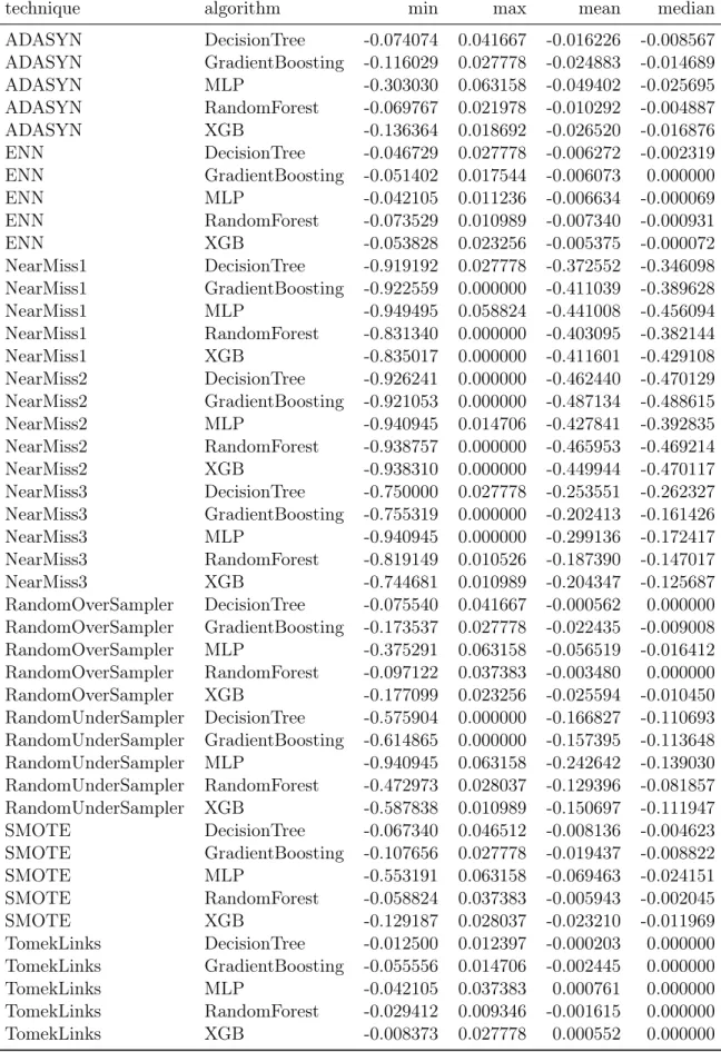
2.6 Differences of F1-score against baseline per algorithm and preprocessing technique 43 2.7 Differences of ROC AUC against baseline per algorithm and preprocessing tech-nique. . . 44
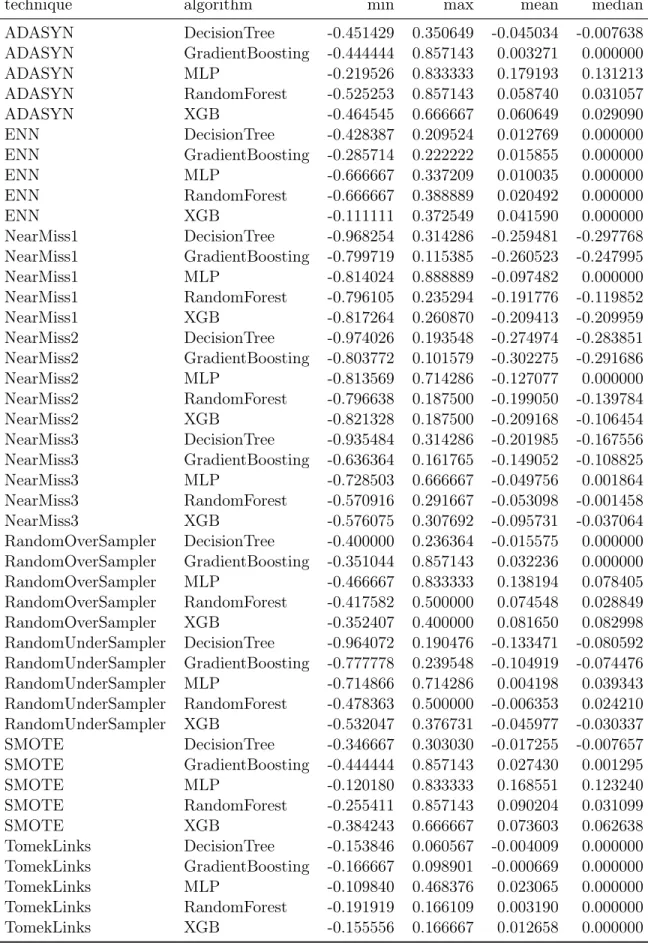
2.8 Differences of Precision against baseline per algorithm and preprocessing technique 45 2.9 Differences of Recall against baseline per algorithm and preprocessing technique 46 2.10 Hyperparameters grid for both vectorizer and classifier . . . 50
2.11 Best parameters for both vectorizer and classifier . . . 50
2.12 Experimental results . . . 52
3.1 Cost Matrix Entries In Binary Classification . . . 55
3.2 Metrics On Test Set Of Different Loss Functions Using Threshold 0.5 . . . 65
3.3 Metrics achieved on the testing set VS the value of β used on the Fβ-Loss . . . 67
A.1 ROC AUC using XGBoost algorithm . . . 74
A.2 ROC AUC using Multi Layer Perceptron algorithm . . . 75
A.3 ROC AUC using Decision Tree algorithm . . . 76
A.4 ROC AUC using Random Forest algorithm . . . 77
A.5 ROC AUC using Gradient Boosting algorithm. . . 78
A.6 Precision using XGBoost algorithm . . . 79
A.7 Precision using Multi Layer Perceptron algorithm . . . 80
A.8 Precision using Decision Tree algorithm . . . 81
A.9 Precision using Random Forest algorithm . . . 82
A.10 Precision using Gradient Boosting algorithm. . . 83
A.11 Recall using XGBoost algorithm . . . 84
A.12 Recall using Multi Layer Perceptron algorithm . . . 85
A.13 Recall using Decision Tree algorithm . . . 86
A.14 Recall using Random Forest algorithm . . . 87
B.1 Improvement of ROC AUC . . . 90
B.2 Improvement of ROC AUC . . . 91
B.3 Improvement of ROC AUC . . . 92
B.4 Improvement of ROC AUC . . . 93
B.5 Improvement of Accuracy . . . 94 B.6 Improvement of Accuracy . . . 95 B.7 Improvement of Accuracy . . . 96 B.8 Improvement of Accuracy . . . 97 B.9 Improvement of Precision . . . 98 B.10 Improvement of Precision . . . 99 B.11 Improvement of Precision . . . 100 B.12 Improvement of Precision . . . 101 B.13 Improvement of Recall . . . 102 B.14 Improvement of Recall . . . 103 B.15 Improvement of Recall . . . 104 B.16 Improvement of Recall . . . 105 B.17 Improvement of F1-Score . . . 106 B.18 Improvement of F1-Score . . . 107 B.19 Improvement of F1-Score . . . 108 B.20 Improvement of F1-Score . . . 109
List of Figures
1.1 Examples of classifiers: Neural Network and AbaBoost, trained against two toy
binary datasets of 2 features each . . . 13
1.2 Example of a convex loss function in a 2-dimensional parameter research space 18 1.3 Example of ROC Curve . . . 24
1.4 Example of Precision-Recall Curve . . . 24
2.1 Distribution of the amount of features per data set . . . 33
2.2 Distribution of the amount of samples per data set . . . 33
2.3 Distribution of the imbalance ratio per data set . . . 34
2.4 Improvements and best values of F1-score, Precision and Recall VS their baselines 41 2.5 Example of Subversion . . . 47
3.1 Architecture Of The Feed-Forward Neural Network . . . 60
3.2 ROC Curves Associated With Different Loss Functions . . . 62
3.3 Precision-Recall Curves Associated With Different Loss Functions. . . 63
3.4 Shapes Of Training Loss (Blue) And Validation Loss (Red) V.S. Epoch Number 64 3.5 Fβ-Loss curves (training in blue and validation in red) corresponding to their value of β . . . 68
3.6 ROC Curves of the Neural Networks corresponding to their value of β in the Fβ-Loss . . . 69
3.7 Precision-Recall Curves of the Neural Networks corresponding to their value of β in the Fβ-Loss . . . 70
Thanks
I want to thank my research director Professor François Laviolette for accepting me as one of his master students. I also want to thank Professor Mario Marchand for giving me advice in terms of reading and having introduced me to the field of Machine Learning. A special thank you must be given to Patrick Dallaire for his support and feedback during the process of writing this very document, and my last year of master in general. Let’s not forget everyone with whom I collaborated over these years, more specifically members of the lab, thank you. On a more personal note, I would like to thank my friends, especially the close ones, for being in my life. Even though it might sound cheesy, this thanks is very real, please take it. Finally, I will never thank Guylaine Gamache enough, but let me try at least: thank you mom for supporting me and loving me since the beginning.
Introduction
In today’s numerical context, data is everywhere and its volume, velocity and variety never stops increasing. We are currently facing a period of time where personal data is acquired by multiple parties to later be used for multiple purposes such as publicity or profiling. As of today’s big data era, it becomes natural for artificial intelligence to play a bigger role, since the three key components to make it possible are now broadly available: efficient algorithms such as deep learning, computational power such as GPUs and cloud computing, and large volumes of data now available from various sources such as digitalization, internet and connected objects. It is common for readily available data not to always be structured and clean. In many situations, the data can be noisy, it may contain missing values or even have duplicates. Data can also present various specificities, even when they are in the same context. For instance, measured characteristics might differ from one source to another, the available amount of data can sometimes be very small or very large, and different types of error can affect the data themselves. A commonly observed phenomenon that regularly results in such problems in data science is the heterogeneity of data (L’Heureux et al.,2017). The data may also have various provenances (geographical, organizational, temporal, etc.), and this information can be very important to consider during training as the data might exhibit different properties depending on the source: some present skewed distributions, some others have a lot of outliers, or some do not exactly represent the same amounts of variables. These specificity of the data, which refers to data quality, is a major challenge in data science.
For predictive tasks, the quality of data can be even more important. In fact, a predictive task’s performance is directly affected by the data itself. For example, the topic of fairness has been increasingly studied in the recent years (Barocas et al. ,2018). This active topic of research attempts to explain and correct potential intrinsic discrimination in prediction tasks, more precisely when the data used for learning contains some forms of hidden biases. This phenomenon is still difficult to measure (Veale & Binns,2017). As a result, it is crucial to keep in mind that relying on data presenting challenging particularities such as the above-mentioned might result in undesirable predictive models.
The present thesis addresses one specific particularity that often affects data quality, which is the class imbalance problem. This problem can be defined as the underrepresentation of
a population with respect to the other populations within a set of data (Japkowicz, 2000). For example, data regarding cancer patients can be very difficult to obtain as opposed to healthy subjects, since the data cannot be actively generated and its collection depends on the healthcare system. The development of a detector for such a task can become very tedious, especially when the total amount of data is limited and no measures are applied to prevent these unwanted biases to impair the learned detector. A broader introduction to the problem will be discussed at the section1.4.
The main goal of the current thesis is to address the binary class imbalance problem. We explore potential solutions, share our findings, and draw conclusions regarding those. The method to achieve this goal will be to realize empirical investigations and practical analysis from both freely available data sets and enterprise case studies. The content is structured as follows:
• Chapter 1 presents a general background on machine learning and on the required
knowledge regarding the class imbalance problem to understand the thesis.
• Chapter 2 presents data preprocessing and resampling techniques used to counter the
imbalance problem, including a case study on the application of resampling techniques to enterprise text data.
• Chapter 3 presents the cost-sensitive learning paradigm, along with works that were
related to its application to neural network loss functions.
• Conclusion presents a summary of what was discussed in this thesis and some future
Chapter 1
Background
1.1
Machine Learning Basics
Machine Learning, which is a subfield of artificial intelligence, is a field of research where the goal is to develop solutions for complex tasks without explicitly programming those. This is done through what we call learning. Actually, learning can be seen as a combination of algorithms and data in order to create knowledge that will later be used to achieve a given task (Mitchell,1997).
To learn, machine learning algorithms require data on which they will train themselves to accomplish their tasks. This data is generally structured in what we call data sets. A data set, as its name suggests, is a collection of data that is organized in a specific way. Usually, this organization of data is to structure it into atomic events or observations. We refer to those individuals in a data set as examples or samples. In particular, we will denote the ith sample of a given data set S as si, which can also be written as follows:
S = {s1, ..., sm},
where m is the cardinality of the data set, or hereafter called the size. It is important to point out that learning algorithms will often rely on statistical assumptions that will ensure their theoretical and statistical validity. The most common assumption is that the examples are drawn from a fixed, common and unknown probability distribution D:
S ∼ D,
where si are iid meaning that they are independent and identically distributed (iid). This
assumption is not always true in reality for many reasons including sampling methodology, temporality and unknown biases in data. However, learning algorithms often succeed to learn regardless of the exactness of the assumptions (Dundar et al.,2007).
One of the most common category of tasks in machine learning consists in making predictions. From this perspective, the development of the predictor is separated into two phases. The first
step of this learning process, most often called the training, consists of making an algorithm learn on the training data. We will usually denote an algorithm A that produces a predictor h using a data set S with:
A(S) → h. (1.1)
The predictor h is usually represented as a function from which its domain and image will vary depending on the type of learning task one is interested in modelling and solving. Once the training phase is completed, we obtain a predictor that can be used for the inference, which consists of predicting pre-specified characteristics on never-seen-before data using the learned predictor.
Indeed, Machine Learning is a very large field of research covering different categories of tasks, which will make s take task-specific forms such as pair of values, vectors, sequences, etc. Depending on the requirements of the task, the learning algorithm is expected to take into account both the task category as well as the provided data structure. In the next sections, we will be briefly introduce the most common categories of tasks encountered in machine learning.
1.1.1 Supervised Learning
Predicting values can be extremely valuable in many applications. For instance, facial recog-nition seeks to predict the identity of a person in an image and this information can be used to make decisions such as granting access to a secure area (Ranjan et al. ,2019). In machine learning, the task that consists in associating a label to an observation is referred to as super-vised learning. From a mathematical standpoint, we are looking to learn a predictor h that is defined on both a domain X and an image Y. The values in the domain X are often called features or inputs, and the values in the image Y are generally called labels or simply outputs. As a result, supervised learning tasks aim to learn a function of the following form:
h : X → Y, (1.2)
where h maps the features in X to labels in Y.
Most of the time, input features are represented using vectors and they will be denoted x. These vectors contain the dimensions of the samples in S that must be used as inputs, which is the very information that will be processed by the predictor to produce the output. Thus, one will usually decompose to each sample si = (xi, yi) as a pair of both features x, and its
associated label y.
Once both inputs and outputs are well defined based on the available dimensions of the data, one can form a training set S of the form:
S = {(x1, y1), ..., (xm, ym)},
containing m samples and use it to learn the predictor (1.2). It is important to point out that h can be modelled in a parametric or non-parametric way, and this will depend on the
type of learning algorithm (1.1) used for training. On one hand, non-parametric predictors rely on the training data itself to make predictions, which means that the main role of the learning algorithm is to determine how the examples are exploited for the inference. In this thesis, however, we will focus on parametric predictors. This has the advantage that we can discard the training examples for the inference, since the knowledge is encoded into a set of parameters θ that will entirely specify the behaviour of h. As we will see in section 1.3, the learning process of those θ can be obtained using optimization techniques such as gradient descent (Bottou,2012).
The spaces X and Y can take various forms, and these forms describe both the nature of the task and the type of learning algorithms to use to fulfill it. For the inputs, it is very common to assume that they belong to some multivariate continuous valued space such as Rdwhere d
is the number of dimensions. This type of input space is typically referred as structured data. Recently, advances in deep learning have made great progress into processing unstructured data such as images and word sequences, and these types of inputs can belong to less common mathematical spaces Henaff et al. (2015), Gheisari et al. (2017). This variety also applies for the outputs. As an example, a label may be as simple as a binary variable (positive or negative) or be as complex as a graph structure, and this depends on the very nature of the problem.
Classification
A problem in which the labels are discrete, but don’t necessarily have an order between each other and describe categories is called a classification problem. A class is described as a possible categorical value for a label y in the domain Y. The simplest variety of classification problems is binary classification. For example, a task where one wants to predict whether someone will purchase a house or not is a binary classification task. As the name suggests, a binary classification problem shows a binary label, such as:
Y = {0, 1}.
The exact labels do not matter as long as they are different to each other and only those two categories exist in the domain Y.
An extension of the binary classification problem to multiple categories is called multiclass classification. Unlike in binary classification, more than two classes exist. For example, in the well known MNIST dataset proposed by Lecun et al. (1998), where one is interested in classifying hand-written digits, the label domain Y is constituted of ten possibilities: Y = {0, 1, 2, 3, 4, 5, 6, 7, 8, 9}. More generally, a multiclass classification problem will put in evidence labels yi such that:
yi∈ {1, ..., K},
It is worth mentioning that one may decide to represent the labels differently than with single values for implementation purposes. For instance, using binary encoding instead of integers is common, both from the practical and mathematical aspects. We will denote the domain Y as follows:
Y = {ek}Kk=1,
such that ek is a K-dimensional unit vector with components ek[j] ∈ {0, 1}and Pjek[j] = 1.
These ek are usually referred as one-hot vectors. For example, the label domain of MNIST
may be represented with the following binary encoding: Y = {e1, ..., e10}.
The one-hot vector representation has the mathematical advantage of orthogonality, i.e. the dot product (or scalar product) between different vectors ek will always be 1 if they are equal
and 0 otherwise. This property is very practical to latter design penalty models (discussed in section 1.2.1). As an example, when the true label is a 5, it would not make sense to give a larger penalty for predicting a 3 and a smaller one for predicting a 4: all mistakes should be equally wrong.
This kind of manipulation of the labels may change the domain Y, but it doesn’t change the problem itself that remains multiclass, because binary encoded vectors still represent single-value labels. This particular encoding is frequently used in classification tasks, because it easily represents categorical data (class labels in this case).
A last kind of classification type is called multilabel classification (Tsoumakas & Katakis,
2009). In this paradigm, an example can belong to any number of classes: all of them, some of them or none of them. That said, using binary encoding of one-hot vectors reveals itself very natural in this context, as an example sees all its classes encoded in a single vector. This kind of classification is a particular case of what we call the structured prediction (or structured output) problem. This field of supervised learning is interested in predicting much more complex labels which are referred here as structures. Other examples of structured prediction problems include sequence prediction (such as part-of-speech tagging (Altun et al.,
2003)), information extraction (such as text parsing (Altun et al. ,2003)) or complex structure prediction (such as protein structure prediction (Liu et al. ,2005)). Even though structured prediction problems are out of scope concerning the present work, they are worth to mention.
Regression
A supervised learning problem where the label domain Y is continuous is generally called a regression problem. That said, Y will usually be a subset of the real numbers R. However, the field of regression can be subdivided into more specific terminology regarding the problem’s domain. First of all, when the labels are real numbers Y ⊆ R, the problem will not have a particular name, one will simply describe it as regression. For example, we could imagine a
regression task where a e-commerce company would be interested in predicting the average of money spent per client based on their individual characteristics or profile.
Another kind of regression is probability regression. As its name suggests, the output domain of the predictor is in the interval [0, 1], because it outputs probability estimations. For this kind of tasks, training and prediction domains are not necessarily the same, because training labels may be binary, for example Y = {0, 1} while the predictions are a probability. It is also possible to re-transform the prediction domain into a binary one using a threshold. A notable example of this kind of task is logistic regression where one uses the logit function (abbreviation for logistic unit or also called sigmoid) to achieve the probability estimation where the finale label will be 1 when the logit function outputs a value above the threshold, and 0 otherwise.
A last kind of regression is ordinal regression (or also ranking learning) (Li & Lin,2006). In this kind of problem, a regression over a given continuous domain is performed to later predict a rank where the predicted value stands in. Ordinal regression can be considered a middle-ground problem between classification and regression, because its effective goal is a classification, however, it performs a regression in order to accomplish it. Moreover, its output class domain does present a natural order (for example {1, 2, 3, 4}) (the word ordinal comes from this fact): the ranks, which correspond to arbitrary ranges that will serve as labels.
1.1.2 Unsupervised Learning
In contrast to supervised learning, the main goal in unsupervised learning is to extract struc-tures in the data. The term unsupervised refers to the particularity that the algorithms will attempt to discover knowledge in data without the need of a supervision, such as the labels used in supervised learning.
Clustering
In unsupervised learning, a frequent task is called clustering. Clustering gets its name from the fact that the algorithms of this family attempt to group examples into what we call clusters, simply a designated name for a collection of samples. These clusters are formed by looking at the features of the examples and the algorithms usually attempt to find patterns in it in order to create boundaries in the data. The algorithm might be based on metrics of similarity (distance) in the feature space (Xing et al. , 2002), (Huang, 2008) and the patterns it finds vary according to the hypothesis it makes based on these metrics. The clusters found during training might later be exploited as estimated labels for further inference.
Density Estimation
A particular form of unsupervised learning is density estimation where one is interested in estimating the density of a given probability distribution by observing examples that have been sampled from this very distribution (Escobar & West, 1995). The ultimate goal of the density estimation is to estimate probabilities p(x) using the estimated density or reproduce the behaviour of the underlying distribution. As the real density of probability of a given distribution cannot be obtained (at least for real world distributions), only approximations can be made and this is the reason the word estimation is used here. This approximation is made by learning to reproduce examples similar to what was previously seen. This notion is introduced here, as it will be tightly related to the notion of data skewness, notion that will be presented later. A possible application of density estimation may be anomaly detection (Laxhammar et al. ,2009).
Dimensionality Reduction
Another common task of unsupervised learning is dimensionality reduction. Some data might present a large amount of dimensions and all of these dimensions may not always be very use-ful for further learning tasks (supervised or not). Moreover, the high amount of dimensions may also decrease performance as it may influence learning into using outliers or anomalies (Verleysen & François,2005). Then, dimensionality reduction tasks usually consist in learning a projection function that will map input data to a more desirable space. Many techniques for dimensionalily reduction exist such as Principal component analysis (PCA) which gets its name from the fact it attempts to find the principal components of the features by using singular value decomposition which projects data to a lower dimensional space (Maćkiewicz & Ratajczak, 1993). For visualization purposes, there exists another non-linear dimensionality reduction technique called T-distributed Stochastic Neighbor Embedding (t-SNE). This tech-nique makes it possible to visualize high-dimensional data in very few dimensions, such as 2 or 3, by building probability distributions over the examples on both high-dimensional and low-dimensional spaces (Van Der Maaten & Hinton,2008).
1.2
Theoretical Foundations
Fundamentally, the very concept of performance is the key goal from which one will choose whether a prediction model is good or not. The definition of the performance of a predictor learned using a supervised machine learning algorithm may vary depending on the finality of the prediction task, however, it can only be quantified through metrics. For example, let’s suppose that one is interested in predicting whether a client is likely to purchase a given product on an online store and learn different binary predictors from historic data. Of course, the learning procedure must be done using a reproducible and valid methodology to obtain an adequate comparison basis. For instance, if a predictor h1 is right 80% of the time on
the testing data while another predictor h2 is right 95% of the time, then most likely h2 will
be a more interesting choice than h1 for predicting the purchasing behaviour. This simple
example is based on a very common metric: the accuracy, which measures the percentage of time a classifier is right on a given testing set. Even though optimizing the accuracy may be the ultimate goal of our experiment in the previous example, machine learning algorithms are not always able to directly optimize a metric using its actual expression; they must use a point-wise (per prediction) equivalent usually called the loss function.
Although many learning algorithms exist and new ones continue to be developed, most of their major components, such as the loss function, are common between each other because they are designed to optimize the performance of resulting predictors. In order to introduce the machine learning field correctly, we must make sure that its common components are well understood. In this section, the loss function will be first discussed to later introduce the concept of risk which represents its global representation. After that, the concept of generalization will be introduced to express the performance at broader level of application. Ultimately, the concepts of hyper parameters and evaluation of metrics will be discussed at a more specific level.
1.2.1 Loss Function
As just mentioned, machine learning algorithms usually make use of what we call a loss function, an important function at the core of the algorithm, calculated per-sample prediction, and used to measure the performance of the learner during the learning process (Rosasco et al. ,2004). Because learning algorithms fundamentally seek to solve a prediction problem
by finding a complex function, the learning process is often modelized mathematically as an optimization problem: the minimization of this very loss function. To summarize, a loss function generally acts as a penalty agent that guides the learning process in the right direction of this optimization process.
Many loss functions exist for different problem and for different contexts. For instance, in a classification context, the most straight-forward example of a loss function is the 0-1 loss defined as such:
L(ˆy, y) = I(ˆy 6= y) where I is the binary indicator function
I(ˆy 6= y) = 0if ˆy = y 1if ˆy 6= y,
L is the loss function, y is the true label, and ˆy a prediction that is produced by a predictor h. For the 0-1 loss, either the prediction is right or not, this means that the penalty effect is applied (if 1) or not (if 0), which is not very powerful, at least not enough for most contexts
of application. In fact, because the loss functions simply represent a penalty, they can be designed very specifically and take various forms.
Let’s take another very frequently used example of loss function, the quadratic loss function, which is defined as:
L(ˆy, y) = (ˆy − y)2.
It is mostly used for regression tasks, but can also be applied to classification in combination with a threshold value. It is commonly called the mean squared error (MSE), especially in the world of neural networks, because it aims to minimize
MSE = 1 m
X
i∈[m]
(yi− ˆyi)2. (1.3)
Unlike the 0-1 loss, which is very strict in terms of penalty, the quadratic loss can express values that are more adaptive to the error of a specific prediction ˆy, and this explains mostly why it is adapted to regression problems.
Another commonly used example of loss function is the log loss which is used to describe a penalty in a probability prediction context (where ˆy is a probability estimation). Its equation looks as follows:
L(ˆy, y) = −(y · log(ˆy) + (1 − y) · log(1 − ˆy)),
for y, ˆy ∈ [0, 1]. Because it takes a probability prediction as input, it is well-fit in a binary classification context where a classifier outputs the probability of the positive label. In case this classifier is a neural network, the log loss is commonly called the Cross-Entropy Loss, because it aims to minimize the measure of cross-entropy:
Cross-Entropy = −1 m
X
i∈[m]
(yi· log(ˆyi) + (1 − yi) · log(1 − ˆyi)), (1.4)
just like the quadratic loss being called the MSE loss.
That said, there exist many loss functions which can be chosen for a given problem. Depending on the nature of the task to achieve, some loss functions will be more adapted than others; for example, 0-1 Loss and Cross-Entropy Loss are more adapted for classification tasks while MSE Loss is more adapted for regression ones. We will also see, in chapter 3, that loss functions can even be constructed specifically for a given task.
1.2.2 Empirical and true risk
The concept of loss function has been described in the previous section, however, the loss function itself is not sufficient to represent the global performance of the model. As loss functions are calculated point-wise, which means for each prediction and not globally (not on a whole given data set), then a larger concept that summarize their values must be introduced: the risk.
Concept of Risk
The risk represents the global error, in other words, it represents the performance that’s miss-ing at a global scale for a given context of application which we represent with our distribution D. To describe it mathematically, let’s take a machine learning setting where we have examples (x, y) that are sampled from a joint probability distribution D over the domains of features X and labels Y:
D : X × Y → R+ (x, y) ∼ D.
Let’s now take a function h that maps features from the domain X to the domain Y: h : X → Y.
Because we want to measure the performance of our predictor h globally for our current setting, we must make the measurement of the loss function described before global. In order to do so, we define the risk R as the expectation of the loss function L which is its integral evaluated on the predictions ˆy of h (h(x) = ˆy) with respect of the joint probability distribution D:
R(h) = E
(x,y)∼D[L(h(x), y)] =
Z
L(h(x), y)dD. (1.5)
That said, we seek to construct an optimal predictor h∗, and this optimal predictor is the one
having the minimal risk. We consider that the predictors h belong to a class of functions H which represents all the possible parametric predictors h ∈ H, whose parameters are denoted θ. This optimal predictor can be written like so:
h∗ = argmin
θ
R(hθ).
This best set of parameters θ must then be obtained through an optimization process. This optimization is usually translated by a minimization of the risk. However, because the real risk itself cannot be measured, the notion of empirical risk will follow.
Why Empirical Risk
As mentioned above, the function h∗ is the optimal predictor we are looking for and this ideal
predictor would describe perfectly the relationship between our domain X and our image Y, because as seen at equation 1.5, minimizing the true risk would permit the closest prediction values according to D. Unfortunately, knowing the exact distribution D over X × Y is not possible in most real-world contexts. However, as seen in the previous subsection, both the mean squared error (1.3) and the cross-entropy (1.4) are examples of risk approximation that can be used as targets.
Because our D is not possible to obtain, neither is our optimal predictor h∗. Despite that, we
approximation is possible because we make the assumption that our data in S is sampled iid from our distribution D. Minimizing the real risk itself still remains impossible, however, a given machine learning algorithm A can minimize an approximation of it:
Remp(h) = 1 m X i∈[m] L(h(xi), yi).
This approximation is called the empirical risk. The empirical risk of a predictor h, Remp(h)
is calculated as the average of the loss function L on the training data S.
The empirical risk minimization (ERM) is the self-explanatory name given to the prin-ciple used to counter the problem of the unknown distribution and true risk, in order to approximate the optimal predictor h∗. The resulting predictor that minimizes the empirical
risk is usually noted ˆh and the ERM, which is used to obtain it, is now probably looking familiar to the reader as two examples of minimization targets were earlier mentioned in the previous subsection: the MSE (1.3) and the Cross-Entropy (1.4).
Generalization
Fundamentally, machine learning algorithms are designed to make use of the data they’re provided in such a way that they will be able to find characteristics from which to discriminate the examples from each other and or discover existing patterns in the data. In real world problems, we are most likely interested in applying inference after the learning phase. Usually, in such a production context, we will have used learning algorithms on real data, not synthetic ones.
In a statistical point of view, we make the hypothesis that the training data S has then been sampled from a real distribution D. However, this data may not represent uniformly this distribution and it is very possible that the resulting regions that are unrepresented in D during learning will as well be unrepresented as prediction candidates during inference. In such cases, we are frequently interested to counter this phenomenon, and it can be expressed in these terms: we want our learning process to be able to generalize well on this given distribution D from the data that was sampled from it.
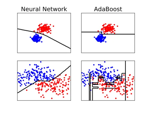
To summarize, if an algorithm generalizes well after using both the training data in the learning phase and the test data at the testing time (when evaluating the model), then it is reasonable to believe its predictions during the inference phase will be mostly following the underlying distribution D and this means that the predictions will also be expected to be close to the reality. An example of two algorithms, one showing better generalization than the other one can be shown in figure 1.1. In this example, the Neural Network algorithm shows better generalization than AdaBoost, because its decision borders (the black lines) present curving lines which fit better the example distributions than the rigid ones of AdaBoost.
Neural Network
AdaBoost
Figure 1.1: Examples of classifiers: Neural Network and AbaBoost, trained against two toy binary datasets of 2 features each
1.2.3 Regularization
Sometimes, training processes may not be able to generalize well in terms of the distribution. Many causes may explain those unsuccessful training processes. One of them is that the provided examples for training might be situated too close to each other in regions of the underlying data distribution. In other words, data provided is too similar and does not represent enough the global distribution.
Overfitting
The previously described phenomenon may lead to what we describe as overfitting, which happens when an algorithm is not able to generalize well and ends up only remembering the examples. This lack of generalization will result in ignoring the true patterns in the data and find entirely random patterns. In other words, a predictor that over-fitted will be able to obtain perfect results if we ask it predictions on the presented training dataset. On the other hand, if we present it new data it has never seen, it will obtain bad performance results. At figure 1.1, we can say that Adaboost has overfitted (at the bottom right), while the neural network seems to have well generalized (at the bottom left).
Unfortunately, this problem of overfitting occurs very easily in most machine learning settings, because the algorithms used to estimate prediction functions usually have a high capacity of
representation. The word capacity, here, refers to the power of a model to represent arbitrary decision functions in a given space. That said, a model being only able to represent an straight line, let’s say the most basic linear separator in a two-dimensional plane, would not be described here as having a high capacity. On the other hand, models such as multilayer feed forward neural networks being able to represent an infinite amount of functions in an arbitrary dimensional space would be. This capacity of representation comes with a cost: the tendency to overfit.
Because overfitting is a common problem that is unavoidable in machine learning problems, techniques have been developed in order to attempt to counter overfitting. We refer to those techniques by using the word regularization.
Many regularization techniques have been proposed and are commonly used depending on which algorithm is being used. For example, in the Ridge Regression algorithm, the Tikhonov regularization (called L2 regularization in machine learning, because it uses the L2-norm)
technique is used. Given a data set S = {(x1, y1), ..., (xm, ym)}, the optimal risk value obtained
by Ridge Regression is shown in the following equation, which uses a weight vector w: min
w
X
i∈[m]
(xi· w − yi)2+ λ||w||22.
We can recognize here that the Means Squared Error (1.3) is the minimization objective of this algorithm, and that the term λ||w||2
2 is the L2 regularization term. This technique essentially
involves adding the euclidean norm of an unknown weight vector to solve from an equation system in attempt to smooth its decision function.
There also exists the L1 regularization, its name also coming from the fact it takes advantage
of the L1-norm. Unlike the L2-norm which is quadratic, the L1-norm is not strictly convex, so
changing only one example in the training set may lead to a completely different solution of w. Hence, the L1-norm is considered less stable than L2. However, because it sums directly
the norms of the weight vectors and not its squares, the regularization effect is weaker, so it is usually more robust to data sets with many outliers. This regularization technique is then more commonly used in conjunction with sparse models.
Another regularization technique commonly used in neural networks is what we call dropout layers. Dropout mechanism involves dropping randomly a certain amount of connecting nodes on a given hidden layer of a neural network during a front propagation iteration. The droppings usually result in a natural regularization effect because of the large percentage of connecting nodes dropped at a given iteration, also considering all dropped nodes are designated on each iteration. Dropout then stimulates resilience in a neural network’s learning process, because of possible strong value changes it generates.
With all the learning components that have been previously discussed, some parameters reg-ulate or control their impact. For example, in the L1 and L2 regularizations that were just
discussed, the λ parameter controls the impact of regularization that is performed on the learned vector. A greater value of λ will increase the effect of smoothness in the learning, so the decision function will be less rigid. At the opposite, a lower value of this parameter will decrease the impact of regularization and result in a sharper, more rigid decision bound-ary. These kind of parameters whose values are not learned during the training process, but rather must be chosen and tuned by the experimenter will be further discussed in the following subsection.
1.2.4 Hyperparameters
Every parameter that controls the behavior of a learning process and than is not learned dur-ing learndur-ing is called an hyperparameter. This name comes from the fact that its value must be chosen a priori, or before the learning. In other words, they are inputs, themselves, to the learning algorithm and they are not limited to numerical values, at a certain point, the choice of an algorithm could be considered as an hyperparameter itself. Common examples of hyper-parameters that are going to be mentioned in this thesis include the λ of regularization, the learning rate of optimizers, the choice of minimization technique (such as Stochastic Gradient Descent in neural networks), the maximum depth allowed to decision-tree-based algorithms, the maximum number of processed features allowed for vectorizing encoders, etc.
The hyperparameters are specific to each algorithm, and some of them are common to many ones, like the regularization λ. Some learning algorithms have many hyperparameters, and as just discussed, the fact of varying their values from one experiment to another may change drastically the results. This is why optimizing their choice is essential to maximize the per-formance. Techniques that permit this optimization will be discussed later, however, because hyperparameters can take many forms, we could simply put them in two main categories: the continuous hyperparameters (the ones consisting of a numerical value, optimizable using ranges, such as λ) and the discrete hyperparameters (the ones chosen directly such as a tree depth or a choice of minimization algorithm).
The discrete hyperparameters are usually more difficult to optimize in terms of computation, because they don’t present a continuous exploration space and all their values usually have to be tried in order to choose the best ones a posteriori. This concept of discrete hyperparameter choice is a key concept here, as the choice of algorithm for data preprocessing is a main goal of the current work, more specifically, the subject of the next chapter (2).
1.2.5 Metrics and Surrogate Losses
Subjectively, one may find it useful to use a model that offers interesting particularities such as training speed, the possibility of training progressively over time, or even the data input capability (the term scaling is commonly used for this purpose). However, in an objective
point of view, any machine learning model must be evaluated in a way that its performance can be measured. In other words, this notion of performance evaluation must be quantified. First of all, many metrics exist in order to measure this performance and evaluating this very performance can be challenging depending on how one considers what this performance is. Choosing the loss that’s equivalent in terms of loss to the main goal metric would be ideal, however this choice is not always possible either because this equivalent function doesn’t exist or because its penalties are too radical. This is why one must choose wisely a loss function that’s adapted to learning and evaluation metrics that are adapted to reflect the performance for the given learning task.
In classification, the mostly known metric is certainly accuracy. As described earlier at the beginning of the current section 1.2, this metric measures the percentage of time a predictor gave the exact right answer, this is where the word accurate comes from. The equation of the accuracy goes as is:
accuracyT(h) = 1 |T | X i∈[T ] I(h(xi) = yi),
where T is a test set s.t. T = {(x1, y1), ..., (xm, ym)}.Of course, sole accuracy is not sufficient
to describe well how a classifier is able to perform on a given test set. Reasons for this will be explained later as the class imbalance problem, which is the subject of this thesis, is a good proof of this claim. Anyhow, metrics are used in the evaluation of models, therefore, we seek to be optimize them to express the performance, which cannot be done directly when the metrics is not differentiable.
The loss functions, presented earlier in this chapter, are used to guide the learning process of a model to optimize in the right direction. That said, sometimes, the objective of learning, the optimization of a given metric or set of metric, cannot be directly expressed in a point-wise optimization fashion, concept that will be later described, or the expression is not powerful enough to update iteratively the learning process in a stable way. In this case, a surrogate loss function is used instead of the direct expression of a metric in its loss form. For instance, the 0-1 Loss is the expression of the accuracy in terms of loss, but this loss function is not used quite often, because it is way too sharp in an update context. As said right before, its penalties are too radical.
1.3
Learning Methodology
Now that learning components common to machine learning problems have been discussed, another important subject rises: common methodology used in machine learning experiments. Even though developing new techniques based on knowledge and reasoning is the basis of algorithmic, including machine learning, using a structured and well defined methodology is essential for reproducibility and comparison. Validity of models and their performances are
usually what is the most important for machine learning algorithms in practice. This is where comparison of models against each other is important. In this section, we will discuss common practices to properly evaluate and compare models.
1.3.1 Model parameters optimization
Because a given parametric model usually presents many parameters, an n-dimensional space, where n corresponds to the amount of parameters, describes ranges from which possible com-binations of values can be picked for these learn-able parameters. From this space, the learning algorithm, must find a combination that will later give the best results according to the loss function. This is why we will generally call this space the search space of the learn-able param-eters. However, the number of dimensions can be very high, hence, it would not be possible to try all the possible combinations. This is why learning algorithms rely on optimization techniques to learn the values of the parameters of their model.
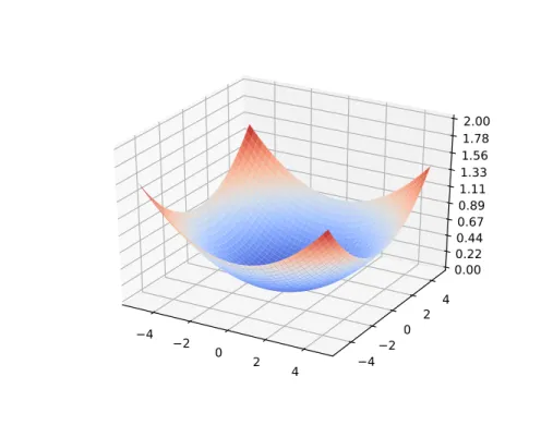
Depending on the model and the loss function, the optimization will differ. For instance, Ridge Regression which was already mentioned makes use of convex optimization, because of its L2-Loss which is convex, ensuring the existence of a global minimum, which once reached,
ensures at its turn that the parameters are optimized. An example of a convex loss function in a 2-dimensional research space is shown at figure1.2. On the other hand, convex optimization is not always possible. For instance neural network algorithms always use non-convex loss functions, instead, they must rely on techniques such as Gradient Descents which essentially consist of following the direction of the gradient in the research space. This is why we generally consider neural networks more difficult to train than convex models.
1.3.2 Model selection & hyperparameters optimization
As discussed in the previous sections, a different choice of hyperparameters versus another one can lead to different results, sometimes very different. That said, it’s natural to expect that one’s goal is to choose the best set of hyperparameters, the set that will lead to the best results possible. As discussed earlier, while the selection of the in-model learned parameters is done using optimization techniques on the loss function, the selection of the model and its hyperparameters are done with the result metrics in mind.
Cross-validation
In order to attain this goal, techniques such as cross-validation exist. This technique involves splitting the training dataset into a series of smaller sets, called folds, and train the given algorithm on the folds but one, which is going to be used to apply a scoring metrics on. This process is repeated in order for each fold to be the scoring one. The hyperparameter set which produced the best score is chosen as the best one and the algorithm is retrained from scratch on the whole training dataset with this very hyperparameter set. This technique is especially
4 2 0 2 4 4 2 0 2 4 0.000.22 0.440.67 0.891.11 1.331.56 1.782.00
Figure 1.2: Example of a convex loss function in a 2-dimensional parameter research space
useful when we don’t have a lot of data, because it permits to validate ourselves without necessarily having a fixed validation data set. Usually, the folds used in cross-validation will be stratified, i.e. they will be grouped in such a way that their amounts of samples per class will be represented in about the same ratio as of the global dataset. Stratification gives usually better results as shown by Kohavi (1995). Cross-validation is often extended in attempt to be more precise, for instance, nested cross-validation is a technique in which each fold is itself cross-validated, but its exhaustive description is out of scope of the current work.
Hold-Out Validation
Another common technique is using a validation dataset. In some contexts, usually where data is abounding, such as when training deep neural networks, performing an exhaustive hyperparameter optimization from a set of ranges like cross-validation is way too heavy in terms of computation. This is the main reason why, most of the time, deep neural networks are not cross-validated. Instead, maintaining a portion of the training data into what we call a validation dataset and using it as an indication of whether the algorithm learns well or not is privileged. This technique is commonly called Hold-Out validation, because a single validation set is literally held out during the whole training phase only for the very purpose of validation. As an example, early stopping is a direct application of Hold-Out validation for neural network algorithms. Early stopping consists of applying a given performance metric on the chosen validation dataset during the learning process and stopping this iterative learning
process when the metric stops improving since the last iteration(s). Usually, the given metric is supposed to improve on each iteration. The premise for this technique is that if the metrics stops improving on the validation dataset, it is explained by the idea that the algorithm’s internal parameters start to overfit on the training data, an unwanted effect.
1.3.3 Model validation
As a last subject but not the least in this section, the validity of the model must be discussed in order to consider whether or not a methodology is right. Training models can be attempted on an arbitrary amount of scenarios, however, in the field of machine learning, some non-written rules that should not be violated exist.
Testing validity
First of all, notcheating is mandatory. The term to cheat, here, refers to looking at the testing set during the training process. Any kind of looking at the testing set from the algorithm’s point of view qualifies to being called cheating, even for a simple purpose of validation, because the model will be considered aware of what it will be tested on. This kind of practice would necessarily compromise the model’s validity because it goes against what machine learning is trying to do: inference on new examples.
Abuse of validation
Another example of non-written rule would be constant prediction functions. That said, imagine a model always predict the same label. This kind of model may be valid in terms of cheating, like previously described, but in terms of learning, certainly not: it has not learned anything. This kind of predictor functions might not be used voluntarily, but rather be ob-tained by an abusive use of a validation data set which can lead consequently to a phenomenon similar to overfitting, but on the hyperparameters, and not the learned parameters. Constant predictions will be reused in the following section as a support to illustrate the imbalance problem, the subject of the current document. Given those concerns, the first thing to do when developing a machine learning model and methodology is to analyze validity of both model and methodology.
1.4
The Class Imbalance Problem
So far, the field of machine learning has been described in a very general way about very technical approaches where experimental context is very well controlled. Nomenclature of machine learning, common learning components and methodology were briefly described in the previous sections and consisted of a basis of knowledge needed to understand the following parts of the document. However, the content of what was described may not apply as is in
an imbalanced context. Even though methodology is a very important aspect of science in general, data is important as well.
1.4.1 Definition of the Class Imbalance Problem
As described earlier, the point of machine learning is actually to learn from some data in order to predict on some more later. In controlled experimental environments, one will generally choose data sets that fit his needs, most likely ones related to the problem he or she is working on. For example, someone working on image classification may use the MNIST dataset, a dataset containing images of hand-written digits (0-9 so 10 classes). He may also use another well known dataset in image classification which is called ImageNet, a dataset containing more than 14 million images divided in about 20 thousand classes. However, those data sets present a common characteristic, they are both fairly balanced. This means that the amounts of samples they contain for each class are relatively close to each other, even though these amounts are not exactly the same. In such experimental contexts, this property of balance is generally present and learning algorithms are therefore developed without worrying about it. However, the property of balance is not always present depending on which data one is using. It is highly possible to have much more examples of one class compared to another one. It is frequently observed. Moreover, this is usually observed for natural distribution reasons. In these contexts, the classes often have an unequal relative importance, meaning that making a prediction mistake on the less abundant class(es) is worst than on the more abundant one(s). Even though this phenomenon seems only like a fact, this is a real problem for machine learning algorithms. Classification algorithms that learn on imbalanced data in terms of class have a tendency to learn much more from the majority class(es) than from the minority one(s). Their discrimination power is then highly affected from it.
An easy solution to this problem may seem to be getting more data. However this solution is not always either possible nor helping, especially in natural-occurrence data. In fact, data is generally assumed to be sampled from an existing distribution, no matter its shape, so it makes sense that most machine learning algorithms usually rely on the iid property of random variables (Independent and identically distributed random variables). Following this principle, getting more data from the same underlying distribution should only increase the amount of examples and reflect more clearly the imbalance, resulting in no help at all, because the very sampling is constrained to iid. For instance, the ratio of patients having cancer in a given hospital will not increase no matter how many times we sample, nor would earth in a given region of land increase its ratio of a particular metal, if we decided to re-sample it indefinitely.
1.4.2 Evaluating performance in an imbalanced context
Another problem related to imbalance is to evaluate a classifier’s performance. To illustrate this problem, giving an example is best. Let’s take a data set S that contains m samples sampled from a joint probability distribution D which its feature space X is arbitrary and its label space Y is binary. Now, let’s suppose we want to learn a binary classifier h(x) : X → Y with S. Moreover, let’s suppose that the number of occurrences of the positive label y = 1 in the data set is about 10%. If we suppose that the sampling was iid, sampling more examples out of it should maintain the current proportion of positive samples of the present joint distribution D. This is also true for another data set T that would be also sampled from D and would be used as a testing set to evaluate metrics on:
1 |S| X i∈[S] I(yi = 1) ≈ 1 |T | X i∈[T ] I(yi = 1).
Then, let’s assume a common methodology where we learn a classifier over the training set S and evaluate the learning process using metrics on the resulting classifier over the training set T. Now let’s imagine a very simple algorithm which builds a constant classifier h according to this rule: h(x) = argmax c ∈ {0,1} X i∈[S] I(yi = c).
Then, in the present example, h results in the constant function h(x) = 0,
because the simple algorithm described just above always builds a constant classifier. It’s certainly no surprise for the reader that the current algorithm could hardly be considered machine learning, it is way too simple and naïve. However, if one looks at the metrics the resulting classifier h could lead to on the testing set, it becomes interesting. For example, let’s consider the accuracy
accuracyT(h) = 1 |T | X i∈[T ] I(h(xi) = yi).
In our case, h(x) = 0, so:
accuracyT(h) = 1 |T | X i∈[T ] I(yi= 0).
Moreover, in our example, we have a T that contains about 90% of samples with a label 0, giving:
accuracyT(h) ≈
1
|T |· 0.9|T | = 0.9.
Recapitulating the example’s context, we have shown that a constant classifier predicting the majority class (that was obtained for instance by a trivial algorithm) can easily perform with
an accuracy close to the proportion of the samples of the majority class in the testing set. This very situation happens frequently in imbalanced context. This is the main reason that only relying on the accuracy or only one metric is not viable, especially in an imbalanced context.
Overview Of Metrics
When facing such an imbalanced scenario, there exist more appropriate metrics than accuracy. Precision and recall (also called sensitivity) are both common examples of those. These two represent respectively a given classifier’s recognition and a retrieval capacity of positive examples. The specificity is the negative-class equivalent of recall. It measures the retrieval power from the negative point of view. These metrics’ expressions are summarized as follows:
precision = T P T P + F P, recall = T P T P + F N, specifity = T N T N + F P, where:
T P =Amount of true positives: examples correctly predicted positive, T N =Amount of true negatives: examples correctly predicted negative, F P =Amount of false positives: examples incorrectly predicted positive, F N =Amount of false negatives: examples incorrectly predicted negative.
The F1-score, described as the harmonic mean of the precision and recall, is another well
known metric. It is useful to obtain a single metric summarizing both precision and recall at the same time. It also has a generalization, the Fβ-score, where the parameter β can be
adjusted in order to give more importance on either the precision or the recall (an higher β putting more weight on recall and a lower on precision). Common expressions of the Fβ-score
are the following:
F1-score = 2precision + recallprecision · recall ,
F1-score = 2 · T P 2 · T P + F N + F P, Fβ-score = (1 + β2) · T P (1 + β2) · T P + β2· F N + F P,
where it is very common to assume a β of 1.
Even though all the metrics already presented help quantifying a classifier’s performance in an imbalance context, they are all thresholded, which means that these metrics are all quantities measured on already made decisions. Fundamentally, many classification algorithms produce a classifier by learning a regressor, which will output a score for each example, and then put
a decision function on top of it in order to decide afterward to which class(es) it belongs. This decision function may be referred to as a threshold in a binary classification context, because it verifies whether a certain score is exceeded to assign an example to the positive class or not (then it belongs to the negative class). As mentioned earlier, the threshold is applied on the output of a regression. This score can also be a probability of belonging to a certain class whenever the score is well calibrated as probability. Even thought there exist metrics that operate on probabilities, this thesis focuses on thresholded metrics.
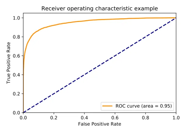
Considering the definitions of the threshold and the score that were just discussed, there exist metrics based on more than one threshold values rather than a single one. A well-known example is the ROC curve, or the Receiver Operating Characteristic curve. This curve maps values of the true positive rate (TPR, another name given to the recall or sensitivity) and the false positive rate (FPR, the opposite of the specificity (1 - specificity)), each of them having an axis (TPR on y-axis and FPR on x-axis). The mapping is obtained by evaluating the given classifier using a large range of different threshold values. Each of these values represent a point on the curve giving both a TPR value and a FPR value. On the ROC curve, a random guessing classifier (such as a coin flip) corresponds to the straight line x = y (or TPR = FPR). Considering this description, a good classifier should present a ROC curve situated above the random guess line. An example of a fairly good ROC curve is shown on the figure
1.3. Moreover, the area under the curve (usually called ROC AUC or simply AUC) is a metric on itself frequently used to summarize a classifier’s ROC curve in a single value.
Another lesser known example of a metric that is not based on one single threshold is the precision-recall curve. An example is shown at figure 1.4. In the same fashion of that of the ROC curve, the precision-recall curve (PR curve) is calculated over a range of thresholds in order to obtain a set of pairs of values associated with threshold values. In this case, the pairs in the PR-curve are values of precision and recall. Even though the PR curve is less popular, it has its advantages. For instance, Saito & Rehmsmeier (2015) propose a study where they conclude that the PR curve is more informative visually than the ROC curve in imbalance contexts. Their claim is supported mainly by the fact that PR curves reflect more easily poor classifier performances than the ROC because the ROC is less sensitive to imbalance compared to the PR. Although its visual information, the PR space, or area under the curve is less useful than the ROC-AUC, mainly because of the curve’s linear interpolation that cannot be easily obtained. This problem was addressed by Flach & Kull (2015) and where they proposes a modification to the PR curve, the PR-Gain curve. Even though interesting, this metric is out of scope of the current work.
1.4.3 Overview Of Current Techniques In An Imbalanced Context
Sometimes, one will use naïve methods in order to tackle imbalance when learning a classi-fier from imbalanced data. Two common examples are randomly duplicating minority-class
0.0
0.2
0.4
0.6
0.8
1.0
False Positive Rate
0.0
0.2
0.4
0.6
0.8
1.0
True Positive Rate
Receiver operating characteristic example
ROC curve (area = 0.95)
Figure 1.3: Example of ROC Curve
0.0
0.2
0.4
0.6
0.8
1.0
Recall
0.0
0.2
0.4
0.6
0.8
1.0
Precision
2-class Precision-Recall curve: AP=0.90
examples or randomly removing majority-class ones. Let’s notice that theses techniques have names, which are respectively random over-sampling and random under-sampling. Even though they may be easily implemented and may suffice for many tasks, they are consid-ered ad hoc techniques and have disadvantages. For instance, removing examples may result in information loss that a learning algorithm could have exploited. On the other hand, dupli-cating examples may result in overfitting because in the lack of diversity in the values of the features in the minority-class.
More sophisticated techniques exist and these approaches may be grouped in three big families:
• Data modification • Algorithm modification • Hybrid approaches
First of all, the data modification approaches are mainly based on the principles of data aug-mentation or data reduction. More explicitly, these approaches either perform over-sampling or under-sampling. These techniques are going to be discussed in the chapter2of this work. Also concerning these approaches, enterprise-related experiments applied to online toxicity de-tection will be presented in the section2.5of the same chapter. After this, approaches based on algorithmic modifications are more diverse. The main approaches regarding this subject that will be discussed in the current work are based on the principle of cost-sensitive learning, a subject that will be more elaborated in chapter 3.
Chapter 2
Data Preprocessing
In machine learning or, more generally, in data science, data preprocessing is a very important subject. A huge amount of the job of a data scientist is in fact to preprocess the data in order to be able to work with it. Data cleaning, structuring, outlier detection, normalization are all parts of preprocessing.
Considering the class imbalance problem, the first family of algorithms that is used to deal with this problem belongs to the subject of data preprocessing. Because the class imbalance problem is a problem coming from the data itself, it’s natural to believe that one may attempt to modify it to solve the problem. This premise is the basis for the algorithms that attempt to “rebalance” data sets before passing them to a machine learning algorithm.
In the current section, the algorithms that will be presented will introduce a notion called resampling. This concept implies that the samples provided to the resampling algorithms will be modified to make it more easily learnable by a later learning algorithm. That being said, as a methodological consideration, the following resampling algorithms are not intended to be used on a whole data set, but on the training data. Hence, these resampling techniques should not be performed on test data, because the test set should be a sample obtained from the distribution for which we want to perform well.
All the resampling algorithms that will be discussed present either a sample generation strat-egy or a sample selection stratstrat-egy (this later for further removal). These strategies, for most algorithms, rely on a concept of distance which is used to calculate examples’ nearest neigh-bours. That said, the KNN algorithm (K Nearest Neighbours) is used by most of the following algorithms in the data feature space.
2.1
Undersampling
The first type of preprocessing algorithms that are going to be discussed are those related to undersampling. This family of algorithms rely on the deletion of examples in order to