Non-destructive data assimilation as a tool to diagnose corrosion rate in reinforced concrete structures
Olivier Anterrieu1, [email protected] (corresponding author)
Bernard Giroux1, [email protected]
Erwan Gloaguen1, [email protected]
Christophe Carde2, [email protected]
1 INRS, Centre Eau Terre Environnement, 490 de la Couronne, Quebec, QC, Canada G1K 9A9 2 LERM SETEC, 23 Rue de la Madeleine, 13631 Arles cedex, France
DECLARATION OF INTERETS: NONE
Abstract: Reinforcement corrosion is a major problem in the long-term management of reinforced
concrete structures. With sustainability in perspective, knowledge of the corrosion rate (Vcor) makes it
possible to estimate the kinetics of the corrosion phenomenon and helps in refining the maintenance strategy of such structures. Although in situ Vcor measurements are possible, data acquisition is
time-consuming because of the protocol intrinsic to its measurement (reinforcement polarization made point by point). Therefore, in the context of site diagnostics, these methods cannot reasonably be used systematically on site and must be combined with high performance non-destructive testing (NDT) surface methods (GPR, capacimetry, half-cell corrosion). In addition, depending on the case, Vcor (point
measurements) and NDT (surface) data are statistically related. However, there is a lack of efficient data assimilation tools permitting accurate translation of NDT data into pseudo Vcor data. In this paper,
we present a numerical tool allowing prediction of Vcor values from NDT measurements. The tool
permits application of different data assimilation techniques, i.e., cokriging, Bayesian sequential simulation, and a decision tree-driven learning depending on statistical behavior and available data. The efficiency of our numerical tool has been tested on a dataset acquired on a structure located in the French Alps. Results show that, for the case study, our data assimilation tool allows prediction of Vcor with accuracy compared to in situ measurements and also permits one to infer the uncertainty of
the prediction. This opens the door for quantitative use of multiple NDT in the management of reinforced concrete structures.
Keywords: Corrosion rate; non-destructive testing; reinforced concrete; data integration; bayesian
sequential simulation; machine learning.
1 Introduction
For reinforced concrete civil engineering structures, corrosion accounts for 80% of observed pathologies and 3-4% of Gross Domestic Product (GDP) in industrialized countries according to the World Corrosion Organization (WCO). When degradations are advanced, repair costs are often very high [1]. Indeed, repair and rehabilitation of structures can sometimes be as expensive as new construction. From a sustainability perspective, it is essential to anticipate the evolution of corrosion phenomenon to optimize the maintenance of structures. The purpose of this optimization is to limit operating losses and to help project owners in infrastructure management and associated costs. It thus appears necessary to promote preventive management at the expense of curative maintenance to wait or lengthen the service life of the structures and to reduce the associated costs [2]. One of the keys for achieving this goal is the assessment of predictable and / or pathological aging phenomena [3]. This assessment must be adapted according to the age of the structure, from preliminary studies to project management, including visual diagnosis, diagnostic measurements and studies.
Because of its basicity (pH ~ 13), healthy concrete is a naturally protective medium. This is due to the presence of a passive film (Fe3O4 - Fe2O3 solid solution) which is formed at the surface of the rebar and which reduces the rate of corrosion to a negligible value. Under certain conditions, such as the carbonation of the coating concrete or a critical chloride content at the reinforcement, this balance can be broken by causing a depassivation of the steel and the initiation of a corrosion phenomenon. In both cases, the destruction of the passive film and the degradation of the metal involve a mechanism of electrochemical cells with anode zones, cathode zones and an electrolytic medium constituted by the interstitial solution of the concrete.
In all cases, corrosion can only develop in the presence of oxygen, which, among other things, explains that the kinetic of corrosion in immersed concrete structures is very low. The two main mechanisms causing the onset of the corrosion phenomenon are the carbonation of the coating concrete in contact with atmospheric CO2 and the penetration of chloride ions from the surrounding environment (marine
environment, use of deicing salts, industrial sites). In the case of carbonation, rebar is depassivated by the decrease of pH to values around 9, caused by the reaction between the hydrates of the cement paste and the atmospheric CO2. The depassivation thus occurs when the carbonation front reaches the
reinforcements. In the case of chlorides, depassivation is initiated when a critical chloride content reaches the reinforcement level. It is accepted that this critical threshold corresponds to a Cl- / OH- concentration ratio of between 0.6 and 1, more conveniently depending on the alkalinity of the concrete, a chloride content of 0.4% in Europe [4] or 0.2% in North America [5], expressed in relation to the mass of cement. It is this value that is retained in the case of reinforced concrete. This threshold is lowered to 0.1% in the case of prestressed concretes. The main impacts of reinforcement corrosion are the development of cracking along the corroded reinforcement, the appearance of abrasions (expulsion of the encasement concrete) and a reduction of the steel section in the mechanically stressed sections.
The two main issues related to the phenomenon of corrosion are to determine the current state (activity, area reached) of the pathology and to evaluate the kinetics of the phenomenon to predict its evolution over time. This is to help the building owners rationalize the resources allocated to repair reinforced structures and minimize the operating loss.
In this perspective of durability of the structures, the measurement of the corrosion rate (Vcor) is
particularly relevant because it makes it possible to quantify the loss of section of the reinforcements as a function of time. The measurement of this property, expressed in μm / year, is based on the analysis of the electrical response of a rebar subjected to a controlled and confined electric field. [6]. The study of the polarization curve makes it possible to estimate the rate of corrosion (Vcor) via Faraday
law, determined from the polarization resistance of the rebar, property representing the capacity of the steel to charge electrically under the influence of electrical impulses.
The main limitation to Vcor measurement is related to implementation constraints in the field (access
to at least one rebar) and acquisition time. Different measuring instruments make it possible to perform point-by-point measurements (a few tens of points / hour) [7]. At the scale of a structure, this extremely time-consuming measure is therefore not economically viable. The measurement of Vcor can
only be piecemeal, so complementary investigation methods (NDT, laboratory analyzes) must be used to complete and make the diagnosis more reliable. The objective of this study is to integrate Vcor point
measurements and measurements from complementary investigation methods to establish maps of the spatial distribution of the corrosion rate. To achieve this goal, four data integration methods are presented and used in this study: NDT fusion, cokriging, Bayesian sequential simulation and decision tree-driven learning.
2 Means of investigation
It is important to distinguish between high-efficiency surface investigation means and point investigation means. These two approaches are however inseparable to establish a diagnosis of the state of corrosion of reinforced concrete.
2.1 High performance surface measurements
To establish a diagnosis of the corrosion state of reinforced concretes, high-efficiency non-destructive testing (NDT) methods allow measuring various indirect parameters that may indicate an environment favorable for the initiation and development of corrosion (weak concrete coating, humidity, electrochemical activity).
For example, GPR method makes it possible to accurately detect and locate the reinforcements within a structure (and thus measure the concrete coating thickness), to reconstruct the reinforcement plane of structural elements (beams, columns, slabs, etc.), to detect voids, and to evaluate, for example, the moisture content of the material [8]. This method is based on the analysis of the travel time and amplitude of high frequency electromagnetic reflected. The travel time and the amplitude of the signals are related to the electrical permittivity and conductivity contrasts of the different materials probed by the wave.
In addition, electrical capacimetry measurements make it possible to locate wet areas within the concrete coating. This method is based on the indirect measurement of the relative dielectric constant of concrete, a property which is difficult to measure but which influences the electrical capacitance (characteristic value of a capacitor in electronics). Knowing that the dielectric constant (ratio of the electrical property of the probed material over the electrical permittivity of empty space) of a common material varies essentially as a function of its water content, it is thus possible to qualitatively determine the spatial and / or temporal variations of humidity within the concrete and to detect an environment favorable to the development of corrosion [8].
Finally, half-cell corrosion measurements are used to qualitatively evaluate the probability of active corrosion of reinforcements in reinforced concrete structures. It is an electrochemical method based on the measurement of the electrical potential difference generated between a reinforcement and an unpolarizable electrode (referred to as the reference electrode - Cu / Cu SO4) displaced on the concrete
surface [9]. By measuring the potential difference according to a predefined mesh, this method allows mapping the active corrosion potential of the reinforcements.
Advances in technology make it possible nowadays to build multi-parameter instruments at reasonable costs, for combined data acquisition on large surfaces offering high-efficiency (> 100 m² / h). Moreover, simultaneous collocated data acquisition eliminates any error in the positioning and implementation of the measurements.
2.2 Additional point measurements
Resistivity is also an indicator of an environment prone to the initiation and development of corrosion. This parameter expresses the transport capacity of the electrical charges and depends mainly on the humidity of the concrete, therefore its porosity, and the possible presence of contaminating salts (especially chlorides). The principle of the method consists of measuring, by means of two electrodes (called potential electrodes), the difference of electric potential (V) generated by the injection of an electric current (I) between two other electrodes (called current electrodes) [10]. Following the Ohm’s law, the resistivity is deduced from the V / I ratio and the geometry of the quadrupole device (Wenner: 4 aligned electrodes, square device, etc.).
Areas of low resistivity (or high conductivity) can contain a high humidity and / or a high salt content (chlorides) and are therefore areas where the risk of active corrosion reinforcements is important [11]. In addition to NDT techniques, point sampling by coring is essential in the realization of a quality diagnosis. These samples by coring allow the realization of physical test (compressive strength, porosity, etc.), chemical (cement, chlorides, alkaline contents) and the assessment of the microstructure.
In addition to providing direct access to the properties of materials through laboratory analysis, this also allows calibrating and correlating measurements from NDT by visually checking the presence and nature of anomalies detected by NDT.
3 Data integration applied to the diagnosis of structures
Conventional characterization of reinforced concrete structures often relies on the separate interpretation of one or several NDT measurements. However, to make the diagnosis more reliable, it is not only necessary to multiply diagnostic variables, but also essential to quantitatively correlate the information collected by the different methods. However, a scientific pitfall exists because the different measured parameters have a large variability in terms of resolution and sampling.
Indeed, point data measurements or primary data (Vcor or laboratory analysis on core samples for
example), are generally expensive to acquire because they are accessible only by tedious measurement (Vcor). However, they are essential to provide direct access to the parameters of the material to be
characterized. So, care must be taken to acquire the minimum amount of primary data without compromising the quality of the diagnostic on spatial distribution of corrosion.
High-efficiency surface data, or secondary data (concrete coating, relative humidity, corrosion potential for example), are accessible through NDT methods and are complementary to the primary data. When compared to the latter, they are much more affordable in terms of cost due to their capacity to investigate much larger surfaces or volumes, but they provide indirect information and need to be interpreted in terms compatible with the primary data.
To jointly exploit these multi-scale and multivariate input data, several probabilistic approaches are described in the literature [12-15]. We propose four different approaches to data integration: NDT fusion, cokriging, Bayesian sequential simulation and decision tree use (supervised learning method).
3.1 NDT fusion / laboratory analyzes
The objective of this integration method is to combine the high-efficiency NDT data and the point corrosion rate data to provide a risk indicator for chloride penetration or carbonation of the concrete mix. Although the penetration fronts of chloride ions and carbonation are complex and happening at different rates depending on location [16], we assume in this approach that these fronts are uniform and parallel to the surface of the auscultated structure.
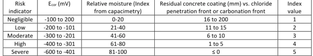
For each parameter obtained by high-efficiency NDT methods, we propose to classify the value according to five different risk indices. The indices range from 1 for a negligible risk, to 5 for a severe, and the corresponding parameter values are presented in Table 1.
Risk
indicator Ecor (mV) Relative moisture (Index from capacimetry) Residual concrete coating (mm) vs. chloride penetration front or carbonation front Index value
Negligible -100 to 200 0-20 16 to 200 1
Low -200 to -101 21-40 11 to 15 2
Moderate -300 to -201 41-60 6 to 10 3
High -400 to -301 61-80 1 to 5 4
Severe -600 to -401 81-100 ≤ 0 5
Concerning corrosion potential data, we first define two thresholds. For the values corresponding to index 1, we choose to combine the potential values recommended by RILEM [17] for dry concrete (0 mV to 200 mV), dry and carbonated concrete (0 mV to 200 mV). mV), wet and carbonated concrete (-400 mV to -100 mV) and wet concrete that does not contain chlorides (-200 mV to 100 mV). Based on the average of these values and our experience acquired in the field, we establish a negligible risk level for the range -100 mV to 200 mV. The corrosion potential data values corresponding to index 5 are also determined by considering the RILEM recommendations for a chloride-contaminated wet concrete (-400 mV to -600 mV). Between these two thresholds, we define a linear gradation of the potential values according to three intermediate risk levels, i.e. a low risk (-200 mV to -101 mV), a moderate risk (-300 mV to -201 mV) and a risk high (-400 mV to -301 mV). Besides, surface relative moisture values obtained by capacimetry can be indexed straightforwardly using ranges proposed in Table 1.
Concerning the concrete coating thickness inferred by high frequency radar (2-3 GHz), the detected surface reinforcement can be associated with an index based on the residual thickness of the reinforcement with respect to the front (carbonation or chloride). To convert GPR data into index values, the depth of the chloride penetration front (or carbonation front) determined by sampling and laboratory analyses is subtracted from the depth of the concrete coating. These residual thickness values are then assigned to index values. For example, if the reinforcement is located at 45 mm depth and samples have shown a chloride front at 20 mm depth, rebar is not affected by chloride front. Then, Table 1 can be used to assign an index value equal to 1 because 45 mm-20 mm=25 mm, which corresponds to a negligible risk.
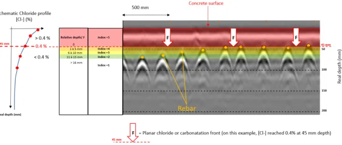
In this case, we assume that the fronts are collinear to the surface even though the fronts are usually irregular. To cope with this uncertainty and to avoid having only two classes corresponding to the affected concrete (index 5) or unassigned (index 1), we introduce three intermediate ranges of 5 mm to the index range (index 2 with index 4) as shown in Figure 1.
Figure 1: Example of reinforcement indexing from a radargram with respect to the chloride infiltration front Each NDT map can thus be converted into an individual risk index matrix, each point of the measurement grid containing values between 1 and 5. It is then possible to weight each index matrix by the Pearson coefficient of the collocated Vcor measurements with those of the NDT. This makes it
possible to consider the influence of Vcor in the integration of NDT data.
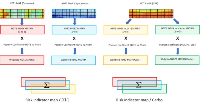
The weighted index matrices can finally be summed up to obtain a global risk index map relating to the influence of chlorides and a risk index map relating to the influence of carbonation. Figure 2 summarizes NDT fusion approach.
Figure 2: NDT fusion approach. Each NDT map (NDT1=corrosion map, NDT2= capacimetry map, NDT3= GPR map) are weighted by the Pearson coefficient of the collocated Vcor measurements with those of the NDT.
3.2 Geostatistical methods
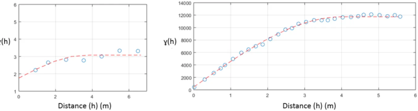
Geostatistical integration methods introduce the notion of regionalized variables. The acquired data is considered to be spatially related. It is possible to determine the importance of the spatial link between two data by evaluating their cross-covariance and modeling it. If a correlation link can be established between collocated primary and secondary data, it becomes possible to estimate the spatial distribution of the primary data based on the spatially evenly distributed secondary data and their cross-covariance and variance. The experimental variogram is commonly used to measure the spatial structure of the correlation of a regionalized variable, i.e., that have a spatial link between them. The blue circles in Figure 3 show the experimental variogram for Vcor and NDT data. The variogram of
stationary regionalized random functions which are the variables that can be processed in geostatistics have experimental variogram that presents a continuously increasing variance (Y-axis) as a function of distance (X-axis) until it reaches a plateau unveiling that the variance of the variable under study is stationary. Once the experimental variogram is computed and has the above mention properties, it needs to be modeled with a variogram function to be used in geostatistical interpolation or simulation algorithms. These functions are characterized by three parameters: 1) the nugget effect which is the variance (Y-axis) at the origin of the distance axis and represent the noise or/and spatial structures that have not been sampled; 2) the plateau or sill that is the variance of the sample data under study; 3) the range, which is the distance (x-axis) at which the variogram reach the plateau. This is particularly interesting for minimizing intrusive and costly primary investigations and reducing associated costs.
Figure 3: Example of experimental variograms (blue dots) and adjusted spherical models (red dashed line) for collocated primary (Vcor - left) and secondary (half-cell potential - right) datasets
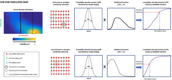
One commonly used method is cokriging, which interpolates the primary variable at any point in the secondary variable's field [18, 19]. This method considers the covariance between all collocated data and has the advantage to strictly reproduce the primary data values at their location when interpolated. The main limitation of this method is the fact that the uncertainty of the data is not considered and that the relation between primary and secondary variables must be linear. To overcome this limitation and thus provide more objective elements of decision support, the Bayesian Sequential Simulation (BSS) method was introduced in the late 1990s [20]. This method has since been applied to solve various problems in the mining and environmental sectors [21-25]. This approach can be summarized as follows.
For a point in the grid of the secondary variable where the primary variable is unknown, the probability density function (P (prim)) can be computed by simple kriging. In the BSS framework, this function is a gaussian defined by its conditional mean (mc) and its conditional variance (Varc). Alternatively, a kernel density estimate can be determined between the primary variable and the secondary variable using collocated measurements [26, 27]. Using the likelihood kernel, a likelihood distribution (P (sec | prim)) can then be determined at the point to be simulated using the values of the secondary variables at that location (the secondary variable is known at this point) between the primary variable and the secondary variable.
Given the law of Bayes:
P (prim)*P (sec|prim) = P ((prim), (sec))
where P ((prim), (sec)) is the joint probability function of the primary and secondary variables. By multiplying the a priori probability density function (P (prim)) by the likelihood function (P (sec | prim)), the posteriori probability function P ((prim), (sec)) of the primary and secondary variables is obtained. By randomly sampling a value from the cumulative density function (CDF) of the posteriori probability function, a value of the primary variable can be simulated. By repeating this process at any point in the secondary data grid following a random path, a mapping of the spatial distribution of the simulated primary variable can be obtained. This approach corresponds to a simulation. Each simulation reproduces the mean and the variance in every way. By reiterating the approach for several simulations (for example 100), we obtain 100 maps of the spatial distribution of the primary variable, whose mean and variance are reproduced in every respect. Figure 4 presents a schematic diagram of BSS.
Figure 4: Schematic diagram of Bayesian sequential simulation
3.3 Decision tree (supervised learning)
This machine learning method aims predicting the values of a parameter (variable response, the rate of corrosion for example) in a study area considering only the data acquired in other areas (predictor data, NDT, chlorides and carbonation depth for example). For this, a database containing the response variable and the associated prediction data must be constructed for different study sites (Study Area SA1 to SAn). Ideally, this database should be the most representative and the widest possible in terms
of geographical location, surveyed structures, pathologies encountered and context (marine environment, cold, temperate, etc.). It is then possible to define one or more decision trees with binary divisions for regression [28, 29]. This tree makes it possible to classify and estimate the values of the response variable in an intelligible manner, considering all the combinations of prediction data available in the database. It thus becomes possible, from new prediction data acquired on a new site SAn+1, to determine the values of the response variable from the decision tree. The database used in
this study includes a dozen of sites on which measurements of NDT, corrosion rate and carbonation have been carried out. These sites are located several regions of France where climatic condition varied (French Alps, South of France, North, etc.) The structures correspond to bridges, cooling towers, etc.
To validate the approach, Vcor values are estimated using regression tree and can be directly compared to the Vcor data acquired on the structure.
4 Application on field example
The four data integration approaches presented in the previous section were tested on measurements acquired on a structure located in the French Alps, allowing access to various types of information useful for decision-making in the context of maintenance. We first describe the study area and the acquired data and then we present the results of the integration methods used.
4.1 Presentation of the study area and acquired data
A NDT measurement campaign was carried out on a reinforced concrete structure located between Geneva (Switzerland) and Chamonix (France) on the Mont Blanc Tunnel motorway (ATMB) in the French Alps. This structure is a lower passage. This structure is 25 m long and about 3 m high. NDT with high-efficiency (radar, capacimetry, corrosion potential) were carried out on the North half span of the structure, in the Geneva to Chamonix traffic direction.
The measurements were conducted on a surface of 12.5 m by 2.5 m in a mesh of 25 x 25 cm. Figure 5 shows photographs of the structure (a) and the location of the study area (b).
(a) (b)
Figure 5: Geometric characteristics of the structure (a) and location of the study area (b) (in green)
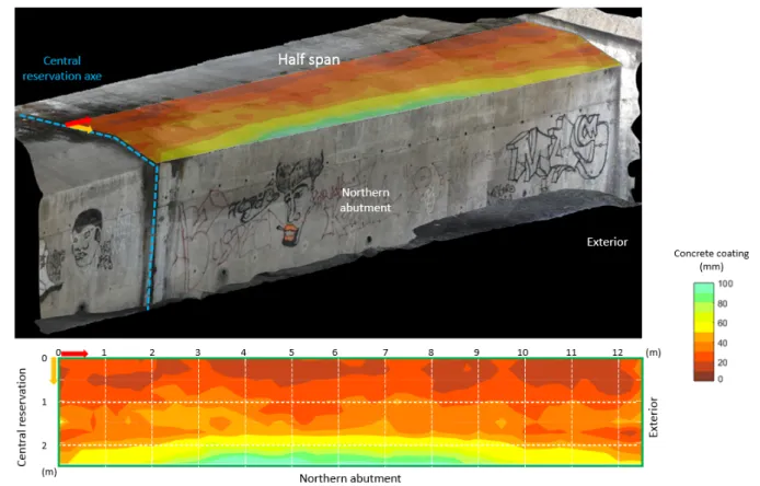
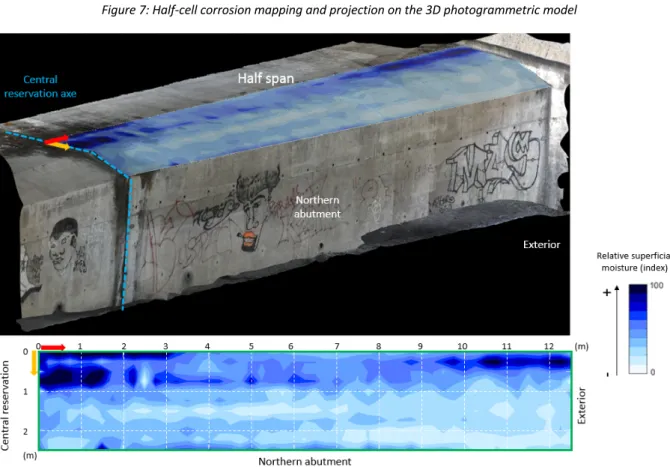
Figure 6, Figure 7 and Figure 8 respectively show the GPR-derived coating mapping, the capacimetric surface moisture mapping and the half-cell corrosion mapping. These are projected on a 3D photogrammetric model of the study area.
Figure 7: Half-cell corrosion mapping and projection on the 3D photogrammetric model
Figure 8: Relative surface moisture mapping and projection on the 3D photogrammetric model
GPR mapping indicates variations in concrete coating thickness. Near the northern abutment, the coating thickness is important (> 50 mm). Moving away from the podium, undercoating areas are observed on the transom. Surface relative humidity mapping indicates wetter areas in the least-coated areas, indicating a favorable environment for the development of corrosion. Half-cell corrosion
mapping confirms this information with significant electronegative potentials highlighted near the central reservation and outward. Note that a zone with electronegative potentials is also highlighted in the right portion of the crossbar.
Thirty point values of the corrosion rate (Vcor) were also measured using a probe developed in the
framework of the DIAMOND project [30] as presented on the 3D photogrammetric model of the study area shown in Figure 9.
Figure 9: Implantation and values of the corrosion velocity measurements (in μm / year) and projection on the 3D photogrammetric model of the auscultated structure
Table 2 presents the correlation coefficients for NDT measurements collocated with Vcor. In addition,
the carbonation depth and the free chloride content were determined in the laboratory. The carbonation depth varies between 5 to 10 mm in the zone. The free chloride content profile is shown in Figure 10. Note that the 0.4% threshold is reached at a depth of about 48 mm. Finally, Table 3 summarizes the main characteristics of measurements made on the structure.
Correlation coefficient Half-cell corrosion/ Vcor -0.8706
Capacimetry/ Vcor 0.3651
Concrete coating/ Vcor -0.1983
Figure 10: Free Chloride Content Profile Measured Near the Central Reservoir Axis
NDT mapping Point NDT Laboratory analysis
Means GPR Capacimetry Corrosion Corrosion rate Chlorides Carbonation Specifications 12.5x2.5 m maps
25x25 cm grid 30 points collocated with some NDT mapping points
7 points
profile Measurement after spraying with phenolphthalein solution Table 3: Summary of the main characteristics of measurements made on the structure
4.2 Results obtained using data integration methods 4.2.1 NDT fusion
Figure 11 and Figure 12 respectively show the results obtained by NDT fusion with respect to the carbonation front and with respect to the infiltration front of the chlorides. From these maps, each class of risk indicator (see section 4.1) can be expressed in m² and as a percentage of the total area investigated as presented in Table 4.
Figure 11 shows a region that can be attributed to moderate to high risk, located near the axis of the central reservation and a region of moderate risk located near the exterior of the structure. The rest of the study area presents a negligible risk. These two regions are also highlighted in Figure 12. The area covered by these regions, however, is larger and a larger portion is classified as high risk. In the center of the study area, another zone corresponding to a moderate risk is highlighted.
Figure 11: Risk indicator obtained by NDT fusion with respect to carbonation and projection on the 3D photogrammetric model (red dot = Vcor data)
Figure 12: Risk indicator obtained by NDT fusion with respect to the chlorides attack and projection on the 3D photogrammetric model (red dot = Vcor data)
Area (m²) / total area Surface (%) Risk/ Vigilance Carbo. [Cl-] Carbo. [Cl-]
Negligible - - - -
Low 25.94 2.17 83 69.5
Moderate 5 6.9 16 22
High 0.31 2.65 1 8.5
Critical - - - -
Table 4: Summary of the NDT fusion results in relation to the size of the area
4.2.2 Cokriging
Figure 13 shows the spatial distribution of the corrosion rate (Vcor) obtained by cokriging with the Vcor
points and half-cell corrosion data (cf. Figure 7) and the projection of the results on the 3D photogrammetric model of the auscultated structure. The regions of moderate to high risk highlighted in the previous figures can be correlated to areas where the rate of corrosion is highest (about 3 to 7 µm / year). Note that at the points of measurement of the corrosion rate (red dots), the cokriged values correspond to the measured values, as expected.
Figure 13: Mapping of Vcor obtained by cokriging and projection on 3D photogrammetric model of the auscultated structure
(red dot = measurement of Vcor)
4.2.3 Bayesian sequential simulation (BSS)
Figure 14 presents the probability maps that the corrosion rate is respectively greater than 1,2,3,4,5 and 6 μm / year, obtained by BSS from the corrosion velocity data and the half-cell corrosion data (see Figure 7). In addition, Figure 15 shows the standard deviation mapping of data simulated by BSS. The spatial distribution of corrosion rates is substantially similar to that obtained by cokriging (see Figure 13). These simulations make it possible to evaluate the results in the form of corrosion rate thresholds and to consider the uncertainty associated with the data.
Figure 14: From top to bottom - probability maps that Vcor is greater than 1,2,3,4,5 and 6 μm / year obtained by BSS (red dot
Figure 15: Standard deviation of data simulated by BSS
As an example, Figure 16 presents the probability map that the corrosion rate is greater than 3 μm /year, projected on the 3D photogrammetric model of the surveyed structure.
Figure 16: Example of probability mapping that the corrosion rate is greater than 3 μm / year obtained by BSS, projected on a 3D photogrammetric model of the structure
4.2.4 Decision tree (supervised learning)
Figure 17 shows the mapping of the corrosion rate obtained by decision tree (supervised learning) and the projection of the results on the 3D photogrammetric model of the structure. The learning database has more than 150 Vcor data points, which are collocated with half-cell corrosion, concrete coating,
capacimetry and carbonation depth data. As previously mentioned, this learning database was built using data acquired on a dozen of different structures, independently of the surveyed structure. In terms of quality, this corrosion rate mapping generally reproduces the anomalies highlighted by cokriging and BSS (see Figure 13 and Figure 14). In quantitative terms, the results estimated by the decision tree are compared with the 30 points of corrosion rate measured on the structure as presented in Figure 18. It is observed that the main trends and orders of magnitude are retained.
Figure 17: Mapping of Vcor obtained by decision tree (supervised learning) and projection on 3D photogrammetric model of
the structure (red dot = Vcor data)
Figure 18: Comparison between onsite Vcor measurements and data estimated using decision tree
4.3 Discussion
The four data integration methods used in the example of this study generally reproduce the same tendencies, which correspond to a localized anomaly near the central reservation axis and a localized anomaly near the exterior of the structure. However, these techniques offer different views to help diagnose civil engineering structures from several angles.
The NDT fusion made it possible to assess globally the state of the surveyed structure by offering a rendering in the form of risk indicator maps. This method made it possible to consider all the NDT data acquired in the study area and the two main mechanisms causing the corrosion phenomenon (chloride attack and carbonation). The risk gradation must be interpreted in terms of vigilance regarding the maintenance of the structure with respect to the corrosion phenomenon. A negligible or low risk will not require vigilance in the short or medium term. A moderate risk will require medium-term vigilance with the possibility of monitoring or additional inspections. High risk will require short-term follow-up with the possible completion of repair work. A critical risk will require the completion of work. This type of integration by NDT fusion can help the structure owners to define a preventive maintenance plan and serve as a guide to prioritize the work areas by quantifying the costs associated with the surfaces to be repaired. The main limitation of the NDT fusion is the classification of the thresholds used to define the risk indices, which can be quite subjective.
Cokriging and BSS were used to characterize the spatial distribution of the corrosion rate (primary variable weakly sampled) considering the spatial with the half-cell corrosion data (densely sampled secondary variable). Cokriging is useful to map the corrosion rate in the field of half-cell corrosion data. The main limitation of cokriging is that it cannot consider the uncertainty of the data. Bayesian sequential simulation made it possible to exploit the results in probabilistic terms by producing several maps of probability of exceeding corrosion rate. This second approach also makes it possible to consider the uncertainty of the data and thus offers the structure owners a decision support tool based on a probabilistic approach. However, the implementation of these two geostatistical methods is dependent on the correlation coefficient between the primary variable and the secondary variable (absolute value of the correlation coefficient must be at least 0.6) and requires enough points of the primary variable to model the spatial link (see section 3.2). Note that in this study, the 30 points of corrosion rate spread over an area of 31 m² allowed to establish a sufficient spatial link to be able to model the variogram. Furthermore, given the correlation coefficients presented in Table 2, only the half-cell corrosion data were used to integrate the corrosion rate data.
The decision tree-driven learning allowed for a mapping of the spatial distribution of corrosion rate considering only a learning database constructed from measurements from other sites (corrosion rate, concrete coating, half-cell corrosion, relative humidity, carbonation depth). Using a learning database of approximately 150 collocated data points acquired on different structures, a decision tree could be modeled by regression. From this decision tree, the corrosion rate has been estimated throughout the study area. The values obtained give orders of magnitude and similar trends to the points where the corrosion rate measurements were acquired. Moreover, the results are broadly similar to those obtained by the other integration methods presented. This highlights the promising nature of artificial intelligence methods in the diagnosis of civil engineering structures. It will be interesting to continue augmenting the learning database from new acquisitions and to model a new decision tree to estimate new corrosion rate values. This is to assess whether the estimated data converges to the measured data as the database is enriched. Table 5 summarizes the advantages, limitations and preferred use of the four data integration methods presented.
Integrated data Benefits Limitations Preferential use NDT fusion
Concrete coating, half-cell corrosion, surface relative moisture, Vcor,
Chloride and carbonation fronts Simplicity of implementation, Consider many parameters
The thresholds defining risk indices are relatively subjective
Mapping a global risk indicator vs. chlorides or vs.
carbonation
Cokriging Vcor + half-cell corrosion Consider the spatial link between the data
Requires enough Vcor data to
model the variogram (cf. 3.2).
Only two variables. Does not account for data
uncertainty
Interpolated Vcor values in
the half-cell corrosion data field
BSS Vcor + half-cell corrosion
Consider the spatial link between the data and
the associated uncertainty
Requires enough Vcor data to
model the variogram (cf. 3.2).
Computationally demanding
Probability maps of Vcor
levels
Decision tree
Concrete coating, half-cell corrosion, surface relative moisture, Vcor,
Chloride and carbonation fronts
Does not require any
measurement of Vcor in
the study area
Requires the widest possible learning database. Stability of the prediction
model (decision tree)
Estimate Vcor values on
structures that do not allow
measurement of Vcor
(difficult access area, survey limited time on site)
Table 5: Summary of the main features of the data integration methods used
5 Conclusions
Four data integration methods were used on a structure located on the Mont Blanc tunnel motorway (France). These methods have made it possible to highlight complementarity of approaches that make the diagnosis of civil engineering structures more reliable.
The NDT fusion is a global integrating tool to provide indicative maps of the damage index to be provided in the maintenance framework. Cokriging may be useful for interpolating spotted corrosion rate measurements in the field of a high efficiency NDT measurement (corrosion potential in this case) provided that a sufficient spatial correlation link can be demonstrated. It also implies a linear relation between primary and secondary variables and it does not to quantitatively estimate the uncertainty. Bayesian sequential simulation can be used under the same conditions as cokriging but offers the advantage of giving access to corrosion rate values in probabilistic terms by establishing thresholds and considering the associated uncertainty. It also permits to handle nonlinear and heteroscedastic statistical relations between secondary and primary variables. It is also convenient to handle multiple secondary variables contrary to cokriging. Finally, the decision tree test made it possible to highlight the value of a superficial learning method to rapidly determine corrosion rates consistent with reality, considering only data acquired from other structures and therefore without even making measurements of this variable in the study area.
Depending on the objectives and the desired rendering (vigilance level map, interpolation of a weakly sampled variable, probability of exceeding thresholds of a variable, estimation of a non-sampled variable from a database) different integration techniques can be relevant and complementary decision support tools for the maintenance of civil engineering structures.
These four integration methods are included in an operating system that is being finalized, allowing not only to integrate multi-scale and multivariate data but also to represent these data on a realistic 3D digital support of the surveyed structure to facilitate their holdings and increase their representativeness.
Acknowledgments
The authors wish to thank the structure owner of the Mont Blanc Tunnel motorway network for the provision of the structure cited as an example in this study, as well as the Laboratory of Study and Research on Materials (LERM, SETEC group) for performing on-site measurements. They also thank the Canadian national research organization MITACS and Setec Canada (SETEC group) for their co-funding of this research.
Bibliography
1. Broomfield, J.P., Corrosion of Steel in Concrete: Understanding, Investigation and Repair, Second Edition. 2006: Taylor & Francis.
2. Ollivier, J.P. and Vichot, A., La durabilité des bétons: bases scientifiques pour la formulation de bétons durables dans leur environnement. 2008: Presses de l'École nationale des ponts et chaussées.
3. Frangopol, D. and Tsompanakis, Y., Maintenance and Safety of Aging Infrastructure: Structures and Infrastructures Book Series. 2014: Taylor & Francis.
4. AFNOR, NF-EN 206-1 - Béton - Spécification, performances, production et conformité. 2014. 5. ACI, ACI 201.2R-16 - Guide to durable concrete. 2016.
6. Andrade, C. and Alonso, C., On-site measurements of corrosion rate of reinforcements. Construction and Building Materials, 2001. 15(2–3): p. 141-145.
7. Alexander, M., Beushausen, H.D., Dehn, F., and Moyo, P., Concrete Repair, Rehabilitation and Retrofitting. 2006: Taylor & Francis.
8. Dérobert, X., Iaquinta, J., Klysz, G., and Balayssac, J.P., Use of capacitive and GPR techniques for the non-destructive evaluation of cover concrete. NDT & E International, 2008. 41(1): p. 44-52.
9. Elsener, B., Andrade, C., Gulikers, J., Polder, R., and Raupach, M., Hall-cell potential measurements—Potential mapping on reinforced concrete structures. Materials and Structures, 2003. 36(7): p. 461-471.
10. Lataste, J.F., Sirieix, C., Breysse, D., and Frappa, M., Electrical resistivity measurement applied to cracking assessment on reinforced concrete structures in civil engineering. NDT & E International, 2003. 36(6): p. 383-394.
11. Balayssac, J.P. and Garnier, V., Évaluation non destructive des ouvrages en génie civil. 2018: ISTE/Hermes Science Publishing.
12. Nguyen, N.t., Nondestructive evaluation of reinforced concrete structures : study of the spatial variability and the combination of techniques. 2014, Université de Bordeaux.
13. Ploix, M.A., Garnier, V., Breysse, D., and Moysan, J., “Possibilistic NDT data fusion for evaluating concrete structures”. DTCE’09, Non-Destructive Testing in Civil Engineering, Nantes, France, 2009. 2009.
14. Sbartaï, Z.M., Laurens, S., Viriyametanont, K., Balayssac, J.P., and Arliguie, G., Non-destructive evaluation of concrete physical condition using radar and artificial neural networks. Construction and Building Materials, 2009. 23(2): p. 837-845.
15. Breysse, D., Klysz, G., Dérobert, X., Sirieix, C., and Lataste, J.F., How to combine several non-destructive techniques for a better assessment of concrete structures. Cement and Concrete Research, 2008. 38(6): p. 783-793.
16. Neville, A.M., Properties of Concrete, Edition : 5, Prentice Hall, Harlow, England; New York. 2011.
17. RILEM-TC-154-EMC, Recommendations of RILEM TC 154-EMC: Electrochemical techniques for measuring metallic corrosion - Half-cell potential measurements - Potential mapping on reinforced concrete structures. Materials and Structures, 2003. 36(261): p. 461-471.
18. Marcotte, D., Cokriging with matlab. Computers & Geosciences, 1991. 17(9): p. 1265-1280. 19. Emery, X., Cokriging random fields with means related by known linear combinations.
Computers & Geosciences, 2012. 38(1): p. 136-144.
20. Doyen, P.M. and Boer, D.L.D., Baysian Sequantial Gaussian Simulation of Lithology with Non-linear Data, W.A.I. Inc., Editor. 1996.
21. Blouin, M., Le Ravalec, M., Gloaguen, E., and Adelinet, M., Porosity estimation in the Fort Worth Basin constrained by 3D seismic attributes integrated in a sequential Bayesian simulation framework. GEOPHYSICS, 2017. 82(4): p. M67-M80.
22. Claprood, M., Gloaguen, E., Giroux, B., Konstantinovskaya, E., Malo, M., and Duchesne, M.J., Workflow using sparse vintage data for building a first geological and reservoir model for CO2 geological storage in deep saline aquifer. A case study in the St. Lawrence Platform, Canada. Greenhouse Gases: Science and Technology, 2012. 2(4): p. 260-278.
23. Dubreuil-Boisclair, C., Gloaguen, E., Bellefleur, G., and Marcotte, D., Non-Gaussian gas hydrate grade simulation at the Mallik site, Mackenzie Delta, Canada. Marine and Petroleum Geology, 2012. 35(1): p. 20-27.
24. Perozzi, L., Gloaguen, E., Rondenay, S., and McDowell, G., Using stochastic crosshole seismic velocity tomography and Bayesian simulation to estimate Ni grades: Case study from Voisey's Bay, Canada. Journal of Applied Geophysics, 2012. 78: p. 85-93.
25. Ruggeri, P., Gloaguen, E., Lefebvre, R., Irving, J., and Holliger, K., Integration of hydrological and geophysical data beyond the local scale: Application of Bayesian sequential simulation to field data from the Saint-Lambert-de-Lauzon site, Québec, Canada. Journal of Hydrology, 2014.
514: p. 271-280.
26. Silverman, B.W., Density estimation for statistics and data analysis / B.W. Silverman. Monographs on statistics and applied probability ; [26]. 1986, London ; New York: Chapman and Hall.
27. Bowman, A. and Foster, P., Density based exploration of bivariate data. Vol. 3. 1993. 171-177. 28. Breiman, L., Friedman, J., Olshen, R., and Stone, C., Classification and Regression Trees. 1984.
FL: CRC Press.
29. Quinlan, J.R., Learning decision tree classifiers. ACM Comput. Surv., 1996. 28(1): p. 71-72. 30. Samson, G., Deby, F., Garciaz, J.-L., and Perrin, J.-L., A new methodology for concrete resistivity
assessment using the instantaneous polarization response of its metal reinforcement framework. Construction and Building Materials, 2018. 187: p. 531-544.