Algorithm for scalar near-field calculations of computer generated holograms

Algorithm for scalar near-field calculations of computer generated hologramss

Stéphane ROOSE

Centre Spatial de Liège, Université de Liège Parc Scientifique du Sart-Tilman, Avenue du Pré-Aily

B-4031 Angleur-Liège, Belgium ABSTRACT

Optical interconnects systems often require the use of computer generated holograms calcukated in the non-paraxial diffraction regime. This paper present the use of the chirp-Z transform algorithm in the calculation of the non-paraxial scalar diffraction problem. The use of this algorithm is memory saving in comparison with convolution with zero-padding. The numerical performances of the approach presented in this paper are comparable with methods using sub-sampled convolution.

Algorithm for scalar near-field calculations of computer generated hologramss

Stéphane ROOSE

Centre Spatial de Liège, Université de Liège Parc Scientifique du Sart-Tilman, Avenue du Pré-Aily

B-4031 Angleur-Liège, Belgium

CGHs with high numerical apertures (F/10<F#<F/2.5 and higher) and high spatial frequencies are required for reasons of compactness in optical interconnects systems. This raises the question about the possible existence of reconstruction errors due to the non-paraxiality that can be superposed on the encoding errors in the the design of CGHs for interconnection purposes. In order to cope with non-paraxiality errors, which are aberrations with respect to the paraxial model (F#<F/10), a more accurate propagation model has to be used. Paraxial complex wavefront synthesis has very often been studied by scientists and it has been shown that it gives relatively good results, as long as one works in paraxial approximations. The Fresnel-Kirchhoff diffraction integral, also called near-field diffraction integral or non-paraxial diffraction integral, is not so widely used due to its numerical complexity.

Nowadays researchers turn their attention to rigorous vectorial diffraction theory applied to the synthesis of CGHs. A rigorous vectorial diffraction theory solves also the problems of non-paraxiality. However the rigorous vectorial diffraction theory is presently only adapted to the analysis and synthesis periodic diffractive structures [1]. Holograms working in the resonance domain, with feature sizes comparable to the wavelength, will have efficiencies that differ from point to point, since this efficiency is dependent on the local spatial frequency, but also on the polarisation. The scalar diffraction theory authorises by no way to make such conclusions on the local diffraction efficiencies and polarisation dependency in the hologram plane. A rigorous vectorial diffraction theory is thus required to describe the light propagation in a small region called the hologram aperture. Once that the vectorial complex wavefront has left the hologram aperture, the polarisation modes remain decoupled and they propagate independently from each other in the free space. Consequently, a scalar theory is sufficient to describe the propagation in free space of these vector components.

The scalar non-paraxial diffraction theory is thus well suited and even required for two kinds of problems: a. design of a CGH in the paraxial regime, calculation of the free space propagation of non-paraxial complex wavefronts from the hologram aperture to image aperture and vice versa.

b. non-paraxial analysis of the diffraction pattern of a CGH designed with a paraxial propagation model.

The free space propagation between a hologram plane and a reconstruction plane can formally be described by:

U(X,Y) = F

exp (i2 d( - f - f ) ) F(u(x, y))

2 y

2 1/2

U

π λ

‰

u(x,y) is the complex signal in the exit plane of the hologram, and U(X,Y) is the complex signal in the reconstruction plane and F() represents a Fourier transform.

A classical numerical method to calculate this is expressed in the following way:

U(o H, p H) = IDFT exp (i2 d( - ( m

H

- ( n

H

) ) DFT(u(o H, p H))

-2 2 2 1/2

∆

∆

U

π λ

)

)

∆

∆

‰

DFT: discrete Fourier transform IDFT: inverse discrete Fourier transform ∆H: sampling rate in hologram plane Η: hologram extent = N∆H

The reconstruction space is sampled at a rate ∆H. If the complete diffraction pattern (I=λd/∆H) has to be evaluated one has to increase the hologram space with zero samples. The fraction between the extent of the reconstructed signal and hologram (I/H) determines the new amount of samples for the calculations. Thus the non-paraxial problem requires a supplementary amount of samples to describe the spatial spread due to diffraction. This supplementary amount of samples requires much more computer memory. The large amount of samples is already one of the major problems in the calculations of computer-generated holograms [2].

One can also put the formal solution into the following form. U(o I, p I) = IDFT exp (i2 d( - ( r

H+ mI) - ( sH+ nI) ) ) CZT(u(o H, p H))

-2 2 2 1/2

r,s

∆ ∆

∑

z

‰

CZT: chirp-z transform IDFT: inverse discrete Fourier transform ∆I: arbitrary sampling rate in reconstruction plane ∆H: sampling rate in hologram plane

In reference [3] one explains the algorithmic details of the chirp-z transform (CZT) algorithm, which was already presented as a solution for scalar paraxial diffraction problems requiring a clever interpolation algorithm. The CZT interpolates the hologram spectrum in subspectra of width (1/∆H) with N samples atv a rate (1/I). Then a sum of Fourier transforms over shifted subspectra is performed and it results in an image of width I. This procedure can be considered as an alternative to sub sampled convolution [4] in non-paraxial diffraction problems. The new algorithm allows to calculate the diffracted field in N by N samples with an arbitrary resolution ∆I.

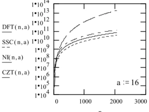
Consider the value a=I/H, as the interpolation ratio. One can make a rough estimate of the number of complex multiplications for the computation of a two-dimensional signal in the non-paraxial regime with diffrent algorithms. 1 104 1 105 1 106 1 107 1 108 1 109 1 1010 1 1011 1 1012 1 1013 1 1014 0 1000 2000 3000 DFT(n a, ) SSC (n a, ) NI(n a, ) CZT(n a, ) n a 16

Fig. 1 Numerical complexity vs. number of samples Fig. 2 RMS-error of an intensity signal reconstructed for 4 types of algorithms, for an interpolation ratio a=16. from a kinoform in the near-field calculated with an

iterative phase retrieval algorithm.

It has been shown that the convolution using a CZT-algorithm is superior based on memory considerations and it allows to implement both forward and inverse diffraction [5]. The speed of the algorithm is of the same order as sub sampled convolution (SSC) and classical convolutions (DFT) with zero padding (See Fig.1). Numerical integration (NI) is generally slower than previous algorithms. (Remark erroneous conclusions where drawn in [5] on the a2 _{dependency in the speed considerations). Due to the accurate} numerical performances it seems that this algorithm might be integrated in encoding procedures such as iterative phase retrieval and error diffusion [5] (Fig. 2).

[1]. E. Noponen, J. Turunen, "Eigenmode method for electromagnetic synthesis of diffractive elements with three dimensional profiles", J. Opt. Soc. Am. A11, 2494 (1994).

[2]. H. Farhoosh, Y. Fainman, S. H. Lee, "Algorithm for computation of large size fast Fourier transforms in computer generated holograms by interlaced sampling", Opt. Eng. 28, 622 (1989). [3]. S. Roose, B. Brichau, E. Stijns, "An efficient interpolation algorithm for Fourier and diffractive

optics", Optics Comm. 97, 312 (1993).

[4]. D.O. Harris, "Efficient computation of near-field diffraction patterns by means of subsampled convolution", Opt. Eng. 33, 175 (1994).

[5]. S. Roose, "Non-paraxial signal synthesis with a CGH", Chapter 5 of "Synthetic holography:

paraxial and non-paraxial signal synthesis with binary diffractive structures", Doctoral dissertation,