Sorting, Incentives and Risk Preferences: Evidence from a Field Experiment

CIRPÉE

Centre interuniversitaire sur le risque, les politiques économiques et l’emploi

Cahier de recherche/Working Paper 06-31

Sorting, Incentives and Risk Preferences: Evidence from a Field

Experiment

Charles Bellemare

Bruce S. Shearer

Septembre/September 2006

_______________________

Bellemare: Département d’économique, Université Laval, CIRPÉE cbellemare@ecn.ulaval.ca

Shearer: Corresponding author. Département d’économique, Université Laval, CIRPÉE bshe@ecn.ulaval.ca

Abstract:

The, often observed, positive correlation between incentive intensity and risk has

been explained in two ways : the presence of transaction costs as determinants of

contracts and the sorting of risk-tolerant individuals into firms using high-intensity

incentive contracts. The empirical importance of sorting is perhaps best evaluated by

directly measuring the risk tolerance of workers who have selected into incentive

contracts under risky environments. We use experiments, conducted within a real

firm, to measure the risk preferences of a sample of workers who are paid incentive

contracts and face substantial daily income risk. Our experimental results indicate the

presence of sorting ; Workers in our sample are risk-tolerant. Moreover, their level of

tolerance is considerably higher than levels observed for samples of individuals

representing broader populations. Interestingly, the high level of risk tolerance

suggests that both sorting and transaction costs are important determinants of

contract choices when workers have heterogeneous preferences.

Keywords: Risk aversion, sorting, incentive contracts, field experiments

JEL Classification: J33, M52, C93

1 Introduction

Contracts play a fundamental role in the economic theory of the firm. Economic theorists have highlighted the ability of contracts to solve moral hazard problems (see, for example, Stiglitz (1975) Hart and Holmstr¨om (1987), Holmstr¨om and Milgrom (1987)) and to reduce transac-tions costs (Barzel, 1989). Recent empirical work has focussed attention on determining the relevance of these contracting models (Prendergast, 2000). Central to this debate is the role of risk and the risk preferences of workers in determining observed contracts. Moral hazard models are based on two premises: individuals react to incentives, and optimal contracts must balance incentives with risk sharing. If risk is important within the contracting environment then observed contracts will vary with risk in predictable ways, giving empirical content to the agency model. However, many studies of actual contracts have failed to detect a role for risk

that is consistent with theoretical predictions; see, for example, Allen and Lueck, 1992.1 These

studies conclude that transaction costs prevent the implementation of optimal contracts, and thus are important determinants of contract choices.

A major difficulty facing empirical work on contracts is that many of the forcing variables are unobservable. Risk aversion, the cost of effort, and, even perhaps, risk itself have no direct observable counterparts. Unobservability greatly complicates testing the theory. Even if risk levels were observable, comparative static results are conditional on unobservable preferences. If workers sort themselves across contracts on the basis of specific preferences, then regression methods seeking to measure the effects of risk on contracts will confound changes in risk with changes in unobserved preferences. This can potentially bias the coefficient estimates and, in turn, downplay the importance of sorting as an explanation of contract choice determination

relative to transaction costs (Ackerberg and Botticini, 2002).2

Perhaps the most direct way to evaluate the sorting hypothesis is to conduct preference-revealing experiments. Such experiments have been used in agricultural economics to

charac-1_{In contrast, empirical studies have produced strong evidence that worker react to the incentives embodied} within contracts; see, Paarsch and Shearer (1999, 2005), Lazear (2000) for evidence based on personnel records and Shearer (2004) for evidence from a field experiment.

2_{An alternative explanation is that firms choose their compensation systems optimally. Prendergast (2000, 2002)} has argued that high-variance environments reduce the efficiency of monitoring inputs, leading firms to use output-based payment systems in these environments.

terize the risk attitudes of farmers (Binswanger, 1980). More recently, Holt and Laury (2002) have developed experimental methods that allow a more precise characterization of risk pref-erences. Their work, conducted within experimental laboratories, suggests that approximately 25 percent of participants are risk-neutral or risk-loving. If sorting arguments can explain the seemingly aberrant estimates of the effect of risk on incentives, then workers who work un-der risky incentive contracts should exhibit behaviour which is consistent with risk-neutral or risk-loving preferences.

In this paper we present direct evidence on the applicability of the sorting hypothesis in the labour market. We exploit data from a field experiment to characterize the risk preferences of a sample of workers who are paid incentive contracts. The experiment, inspired by the work of Holt and Laury (2002), was conducted within a tree-planting firm operating in British Columbia, Canada. The workers of this firm are paid piece rates and face substantial daily earnings risk due to random planting conditions.

Our results suggest that a significant proportion of the workers in this firm (between 39% and 46%) were risk loving or risk neutral. These figures are considerably higher than existing results from experiments performed on broader populations; see, for example, Holt and Laury (2002) and Elston, Harrisson, and Rutstr¨om (2005). We find no evidence to suggest that mea-sured risk preferences are related to past accumulated earnings (productivity), age, or gender. We also show that our results are not sensitive to the payoff scales used in the experiment. We argue that these results provide support for the sorting argument: contracts that expose workers to risk, attract workers who are risk-tolerant. Consequently, empirical work aiming to uncover the relationship between risk and contracts by considering different classes of risk-bearing contracts, must account for sorting.

The rest of the paper is organized as follows. The next section provides institutional details of the tree-planting industry in British Columbia. In section 3, we present the experimental design. In section 4, we present and analyse the data. In section 5, we discuss the implications of our results and conclude.

2 Tree Planting in British Columbia

While timber is a renewable resource, active reforestation can increase the speed at which forests regenerate and also allows the control of species composition. In British Columbia, extensive reforestation is undertaken by both the Ministry of Forests and the major timber-harvesting firms.

Tracts of land that have recently been logged are allocated to tree-planting firms through a process of competitive bidding. These auctions typically take place in the autumn of the year preceding the planting season, which generally runs from early spring through to late summer. Tree-planting firms submit bids over the price per tree (or bid price) that they will receive to complete a given contract. These bids are calculated after having observed the planting con-ditions (eg. the slope and rockiness of the terrain) on the land to be planted. These concon-ditions affect the number of trees that can be planted in a given day and therefore affect labour costs. The lowest-bidding firm wins the contract, returning to the site the following year with hired workers to plant trees.

Tree planting is a simple, yet physically exhausting, task. It involves digging a hole with a special shovel, placing a seedling in this hole, and then covering its roots with soil, ensuring that the tree is upright and that the roots are fully covered. The amount of effort required to perform the task depends on the terrain on which the planting is done and weather conditions. Flat plateaux are much easier to plant than steep mountain sides and hard, rocky soil is more difficult to plant than soft terrain. British Columbia is a very mountainous region of Canada; the terrain can vary a great deal from site to site.

Planters are predominantly paid using piece-rate contracts, although fixed wages are used

on occasion.3 _{Under piece-rate contracts, planters are paid in proportion to their output.}

Gen-erally, no explicit base wage or production standard exists, although firms are governed by minimum-wage laws. Output is measured as the number of trees planted per day.

3_{See Paarsch and Shearer (2000) for a discussion of when firms use fixed wage contracts and the effects of these} contracts on worker productivity.

2.2 The Tree-Planting Firm

Our experiment was conducted within a medium sized tree-planting firm that employed a total of 78 planters in the 2005 planting season. The planters represent a very broad group of individuals, including returning seasonal workers and students working on their summer holidays. They range in age from 19 to 56.

This firm pays its planters piece rates, exclusively; daily earnings for a planter are deter-mined by the product of the piece rate and the number of trees the planter planted on that day. Blocks to be planted typically contain between 20 and 30 planter-days of work, with some lasting over 100 planter-days. For each block, the firm decides on a piece rate that applies to all planting done on that block. Planting conditions vary across and within blocks. For exam-ple, while a given block may be appear uniform on the surface, some parts of the block can be characterized by rocky soil under the surface, making planting more difficult. Given the firm cannot completely know the undersoil conditions for the whole block, some planters will in-variably end up working in more difficult conditions, under the same contract. These random elements expose planters to daily income risk.

Contracts, comprising a number of blocks in the same geographic area, are planted by crews of workers under a supervisor. Each crew typically has from 10 to 15 planters. All workers planting on the same block receive the same piece rate; no matching of workers to planting conditions occurs. Typically, planters are assigned to plots within a block as they disembark from the ground transportation taking them to the planting site. Thus, to a first approximation, planters were randomly assigned to plots.

2.3 Earnings Risk

Table 6 presents descriptive statistics for the 2005 planting season for planters who participated in our experiment. The average daily number of trees planted is 833.94, with a large standard deviation (426.08). The average daily earnings is $196.12 with a standard deviation of $66.43. Planters have, on average, worked 21.36 days before taking part in the experiment, again with a sizeable standard deviation. It is possible to decompose the total variation in productivity in one part due to differences in productivity across planters and another part reflecting

differ-ences in daily planting conditions.4 We find that 57.1% of total variation in daily productivity can be explained by variations in day-to-day planting conditions, while 42.9% of the total vari-ation is accounted for by productivity differences across planters. Similar results apply when we look at daily earnings. We find that only 39.2% of the total variation in daily earnings re-flects variation in productivity across planters. This implies that 60.2% of the daily variation in earnings (a standard deviation of approximately 51$) can be attributed to daily variation in planting conditions and piece rates, indicating considerable earnings variability beyond the planters’ control.

3 Experimental design

The field experiment took place on five consecutive mornings during the first week of May, 2005. Each morning, we met with a different crew of planters for approximately twenty minutes before the crew set out to their planting site. The size of the crews varied from day to day, rang-ing between 5 and 25 planters.

To begin, we introduced ourselves as economists conducting a study on the behavior of workers in the presence of risk. The planters were informed that they would receive a 10$ fee for their participation in this study, plus an additional sum which would depend on the choices they made and chance. Participation was voluntary. Each planter who agreed to participate

was given paper instructions, a decision sheet, a clipboard, and an ink pen.5 _{We then read}

aloud the instructions on the experiment and on how to fill in the decision sheet. We used an oversized copy of the decision sheet to assist us in describing the experiment.

To complete the experiment, each planter had to make 10 decisions. Each decision consisted

4_{The decomposition is based on the following model of daily productivity y} it

yit=α+µi+εit

where α is an intercept, µirepresents fixed planter-specific, time-invariant productivity effects, and εitrepresents other unsystematic differences in planting conditions. Under the assumption that µiis independent of εit, the total variance in y_itis given by

V(yit) =V(µi) +V(εit)

The share of the total variance due to day-to-day variation in planting conditions is simply V(εit)/V(yit). 5_{There were no cases of planters refusing to participate.}

of choosing one of two binary lotteries. A summary of the decisions can be found in Table 2. The actual decision screen is presented in appendix A. The lotteries used were inspired by the experimental design developed by Holt and Laury (2002) to determine the risk aversion of an individual. For each decision there is a ”safe” lottery, denoted A, which pays either a low payoff of $16.00 or a high payoff of $20.00, and a ”risky” lottery, denoted B, which pays either a low payoff of $1.00 or a high payoff of $38.50. Which of the high or low payoffs materialized, was determined by chance.

For the first decision, the probability of the high payoff for both lotteries is 10%, so only an extreme risk seeker would choose lottery B. As can be seen in the far right column of Table 2, the expected payoff difference between lotteries A and B, for the first decision, is $11.70. The prob-ability of winning the high payoff increases gradually as we move down the Table, increasing the relative payoff of the risky lottery B. Consequently, an individual should eventually cross over and start choosing lottery B as he/she moves down the decision sheet. In fact, for the last decision, the high payoff of each lottery is paid with probability 1 ($20 for lottery A, and $38.50 for lottery B). This means that even very risk averse individuals should choose lottery B in the last decision.

The pattern of decisions for a given planter can be related to existing utility functions rep-resenting preferences over risk. With constant relative risk aversion for money x, for example,

the utility function is u(x) = x1−r_{for x >0 and where r denotes the coefficient of relative risk}

aversion. This specification implies risk loving behavior for r<0, risk neutrality for r=0, and

risk aversion for r > 0. The payoffs for the lottery choices in the experiment are such that the

crossover point from lottery A to lottery B provides an interval estimate of a subject’s coeffi-cient of relative risk aversion. The payoff numbers for the lotteries are such that a risk neutral decision pattern (four safe choices followed by six risky choices) is consistent with a constant relative risk aversion coefficient r in the interval (-0.15, 0.15). Similar intervals can be obtained for other functional forms of utility, namely constant absolute risk aversion.

After we described the decisions they would be making, planters were informed that, once their decisions were made, one of their ten decisions would be randomly chosen and played out to determine their earnings. To select which of the ten lotteries would be played, each planter would first draw a poker chip from an opaque, black bag, containing identical chips numbered from 1 to 10. The number drawn would select the lottery to be played. We would then replace

the chip in the bag, shuffled the bag, and ask the planter to draw a chip for a second time, this

time to determine the outcome of the selected lottery, and thus the planter’s lottery earnings.6

Planters were informed that their lottery earnings and participation fee would be added to their next pay check. After having read the instructions, participants were allowed to ask clarifying questions. We then asked each planter to make their decisions individually and in silence. Planters who completed their decision sheets were asked to come forward to draw their poker chips.

Each daily session took on average 15 minutes. In total, all 51 planters of the firm who worked during that week participated in the field experiment. The average earnings during the experiment (which took approximately 20 minutes of the planter’s time) was $30 (including the participation fee). Since average daily earnings was approximately $200 for an eight-hour day, the average experimental earnings is just under four times what a planter could expect to earn in a twenty-minute spell of planting. Moreover, the difference between the high and low payoffs in the risky lottery B (37.50$) is just under a one standard deviation in observed daily earnings risk (51$, see Section 2.3). Consequently, the experiment represents considerable payoffs to the planters, and the risky lottery offers a realistic variation in earnings.

4 Results

Table 3 presents the results of the experiment. The first column indicates the number of safe choices made in the experiment. The second column presents the interval around the coefficient of relative risk aversion r which is consistent with a given number of safe choices. The third column presents the typology used by Holt and Laury (2002) to classify risk preferences. As can be seen from the Table, risk neutral individuals should choose 4 times the safe lottery before crossing over and choosing the risky lottery. Risk loving individuals make less than 4 safe choices, while risk averse planters make more than 4 safe choices. The fourth column presents the cumulative distributions of the number of safe choices made in the baseline experiment for

6_{For example, a planter who selected the number 4 on his first draw would play lottery A.4 if he had selected} lottery A for decision 4 and B.4 if he had selected lottery B. If his second draw was in the interval 1-4, he would win $20 if he had selected lottery A and $38.50 if he had selected lottery B. If his second draw was in the interval 5-10, he would win $16 if he had selected lottery A and $1 if he had selected lottery B.

all 51 planters. The fifth column presents the cumulative distribution of the number of safe

choices only for planters who gave consistent answers.7

We find that 39.2% of tree planters have risk aversion profiles between extreme risk loving and risk neutral, and 72.6% have risk profiles between risk loving and weak risk aversion. These probabilities tend to increase when we exclude planters who gave inconsistent answers. These results show a significant level of risk tolerance among these workers.

The proportion of workers exhibiting risk tolerant behaviour is much higher than in studies sampling individuals from broader-based populations. Holt and Laury (2002) performed sim-ilar experiments on university students. They found that approximately 25% of their sample displayed risk preferences between risk loving and risk neutral. Harrison, Lau and Rutstr¨om (2005) found that approximately 23% of subjects randomly drawn from the Danish population have risk preferences between risk loving and risk neutral. The higher proportion of incentive-pay workers displaying risk-tolerant preferences is consistent with the sorting hypothesis –

high-powered incentive contracts attract workers who are tolerant to risk.8

4.1 Income Effects

One possible confounding effect for the relatively low incidence of risk aversion in our sample is that planters vary in their level of seasonal earnings, with some planters having begun work early in the season, thus having accumulated substantially higher earnings. Greater earnings has long been believed to foster risk-seeking behavior. If this was the case, then we should observe a negative and significant relationship between accumulated seasonal earnings (up

until the day of the experiment) and the number of safe choices made in the experiment.9

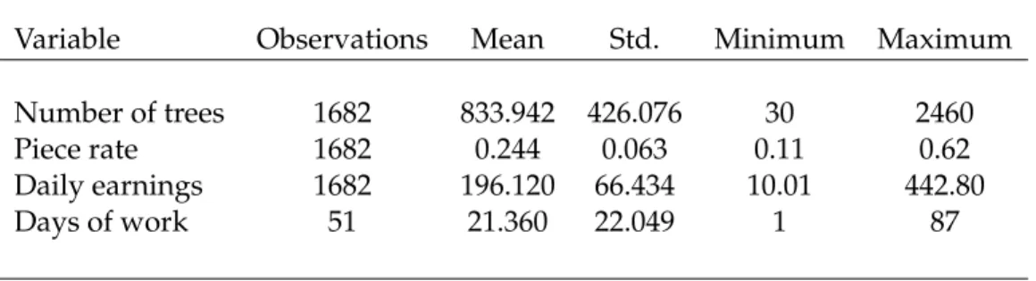
Using payroll data from the firm, we were able to test the null hypothesis that accumu-lated seasonal earnings does not significantly explain risk taking behaviour in our experiment. Figure 1 presents the past accumulated earnings of planters who took part in the experiment as a function of the number of safe choices made in the experiment. We do not find a clear

7_{Inconsistent answers consisted of planters crossing more than once between lotteries. The percentage of} planters giving inconsistent answers was 31.2%. Holt and Laury (2002) report that approximately 15% of students made inconsistent decisions when first playing such an experiment.

8_{We discuss this point further in Section 5, below.}

9_{Evidence of income effects when measuring risk aversion has not been observed in laboratory experiments with} student samples (see Holt and Laury (2002)).

relationship between earnings and the number of safe choices made.

To investigate whether the dispersion in past seasonal earnings of planters is systematically related to other factors, we use regression techniques developed for count data. In particular,

let N be the number of planters, and s_i ∈ {0, 1, ..., 10} denote the number of safe decisions

(choices of lottery A) of planter i, where i = 1, 2, ..., N. We model si as a Poisson process with

conditional mean

(1) λ_i(x_i) =exp¡x_i0β¢

where β denotes a vector of population parameters, and xi denotes a vector of characteristics

including accumulated earnings, a quadratic in accumulated earnings, the number of days of planting in the current season up until the experiment, a binary variable indicating whether the planter made consistent decisions in the experiment, and personal characteristics: age and

gender. The likelihood of observing a number of safe decisions S equal to si, conditional on xi,

is given by

Pr(S=s_i|x_i) = e

−λi(xi)λ

i(xi)si s_i!

Estimates of β are obtained by maximizing the sample log-likelihood function

(2) 1 N N

∑

Table 4 presents the regression results with standard errors in parentheses10

These results suggest that our measure of risk aversion is unrelated to income effects. In particular, we find no evidence of a linear or non-linear relationship between measured risk aversion and past cumulative earnings. These results hold whether or not we condition on the number of days worked until the day of the experiment, on whether or not planters made consistent decisions in the experiment, and on whether or not we condition on age and gender. One of the possible reasons for the lack of statistical significance in Poisson regressions is due

10_{A well known restriction of the Poisson regression model is that the conditional variance of s}

ishould equal the conditional mean given in (1). Gourieroux, Monfort and Trognon (1984) have shown that consistent estimates of β can be obtained by maximizing (2) even if the conditional variance differs from λi(xi)as long as the conditional mean is well specified. Consistent estimates of the covariance matrix of parameter estimates can than be obtained using the robust sandwich estimator (see Gourieroux, Monfort and Trognon (1984) for details).

to under dispersion, which occurs when the conditional variance is lower than the conditional mean. We tested the null hypothesis of no under dispersion for all for regressions presented

in Table 4.11 The results are presented in the last row of Table 4; we do not reject the null

hypothesis in any of the four specifications.

4.2 Scale effects

Recent research suggests that the distribution of measured risk aversion is not independent of the scale of lottery payoffs. In particular, measured risk aversion tends to increase when

payoffs are increased (Holt and Laury (2002, 2005)).12

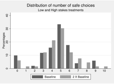
To investigate whether our results are affected by payoff scales, we conducted a follow-up experiment, involving 66 planters, with higher payoffs. This follow-follow-up experiment was conducted in the spring of 2006, a year after the initial experiment was completed. 18 of the 51 planters who participated in the baseline experiment participated in the follow up experiment. The payoffs in the follow-up experiment were double the payoffs from the initial experiment. Hence, the safe lottery, A, now paid either 40$ or 32$, while the risky lottery, B, now paid 77$ or 2$. As in the baseline experiment, each planter received a 10$ participation fee in addition

to their earnings. Once again, all planters participated.13

Figure 3 presents the distribution of the number of safe choices under both payoff scales. Somewhat surprisingly, we find both distributions are very similar. There are, perhaps, two noticeable differences. First, increasing the payoff scale seems to cause a slight shift from weak risk aversion (5 or 6 safe choices) to risk neutral and weak risk loving (3 and 4 safe choices). Second, the proportion of planters making no safe choices slightly decreases when the payoff

11_{The test statistic is based on the auxiliary regression} ³ si−bλi(xi) ´₂ −si b λ_i(x_i) =αbλi(xi) +εi

where s_iis the number of safe decisions of planter i, bλ_i(x_i)denotes the predicted conditional mean, ε_iis an error term, and α is a slope parameter. The t statistic for α is asymptotically normal N(0, 1)under the null hypothesis of no under dispersion. See Cameron and Trivedi (1998) for details.

12_{One implication of this is that a large class of preferences (e.g. CRRA), which are insensitive to payoff scales,} are inappropriate approximations of risk preferences.

13_{There were more planters in the firm in 2006 than in 2005, explaining the difference in the number of} partici-pants.

scale is increased. Table 5 compares the cumulative distribution of the number of safe choices in the baseline and follow up experiments. We see that the proportion of planters who are either risk neutral or risk loving slightly increases relative to the baseline treatment (42.4%). As in the baseline treatment, risk aversion appears to decrease when restricting the analysis only to planters which gave consistent answers.

To further investigate differences in behaviour between the two payoff scales, we conducted chi square tests on the distributions of measured risk preferences under the low and high payoff

scales.14 _{The null hypothesis states that the two distributions of measured risk preferences are}

from the same population. The chi square tests do not reject the null hypothesis – this, whether we compare all planters in both treatments (p-value = 0.428), or whether we compare only planters who gave consistent answers in both treatments (p-value = 0.454).

It is possible that by expanding the firm (to 66 employees), the firm hired a group of risk-lovers and this counteracts the change in risk-preferences of those who participated in both experiments. While this possibility would provide additional evidence in favor of sorting, it also potentially complicates testing for scale effects. One way to control for this effect is to compare the distributions of the number of safe choices for those 18 planters who took part in both experiments. This way, the sample of planters used to perform the comparison remains fixed. Again, a chi square test (p-value = 0.352) is unable to reject the null hypotheses that the distributions in the baseline and follow up experiments are the same for these planters. Consequently, we conclude there is no significant evidence that our results are affected by

these changes in payoff scales.15

5 Discussion

To better appreciate the levels of risk tolerance exhibited among these piece-rate workers, we compare our results to those found for other populations. We focus on studies which have

mea-14_{The test statistic is given by(pb}

l−bph)0Vb−1(bpl−pbh)where bpland bphdenote 10 by 1 vectors of estimated pro-portions of planters making 0,1, ..., and 9 safe choices in the low l and high h payoff experiments and bV−1_{is the} estimated variance of(bp_l−pb_h). The asymptotic distribution of the statistic is chi square with 10 degrees of freedom under the null hypothesis that both distributions are the same.

15_{We also performed all our tests using the nonparametric Mann-Whitney rank sum test of the null hypothesis of} equal medians. The estimated p-values were consistently above 0.80% in all cases.

sured risk preferences using the Holt and Laury instrument with similar payoffs. Using similar payoffs avoids the problem that subjects from other studies appear more risk averse when the lotteries involve high payoffs (see Holt and Laury, 2002). First, we compare our results with those obtained by Holt and Laury (2002) on a student population. We use parameter estimates reported in their paper to predict the proportion of safe decisions their students would make

under our baseline lottery payoffs.16 _{Second, we compare our results to those in the study by}

Elston, Harrisson, and Rutstr¨om (2005) who measured the risk preferences of entrepreneurs and salaried non-entrepreneurs using the Holt and Laury instrument. Their payoff scale per-fectly matches the one in our baseline experiment (see Table 2), so we can directly compare results. They find that salaried non-entrepreneurs are significantly more risk averse than full-time entrepreneurs. We focus here on the decisions made by the full-full-time entrepreneurs, since this reduces the odds that tree planters appear relatively more tolerant to risk.

Figure 2 graphs the proportion of subjects choosing the safe lottery (vertical axis) versus the decision number corresponding to the rows in Table 2. Higher decision numbers correspond to increases in the attractiveness of the risky lottery relative to the safe lottery; i.e., as we move down Table 2. A risk-neutral subject would choose the safe lottery for the first four decision numbers, before switching to the risky lottery for the remaining decision numbers. Only risk loving individuals would not chose the safe lottery in any of the first three decisions. The predicted proportions for students choosing the safe lottery for the first three decisions is very close to the risk neutral prediction. In the population of full time entrepreneurs, approximately 90% percent of subjects opted for the safe lottery in the first three decisions, an indication that that full time entrepreneurs have a stronger tolerance for risk than do students. Only between 76% and 80% of the tree planters who took part in our field experiment opted for the safe lottery in one of the first three decisions, numbers which are significantly lower than for entrepreneurs and students. As expected, the proportion of subjects choosing the safe lottery diminishes in the three samples as the decision number increases. More importantly, the proportions playing

16_{They fit a power-exponential utility function which can account for the effect of changes in payoff scales present} in their design. The power-exponential function over stakes x is given by U(x) = (1−exp(−αx1−r))/α. It can be shown that constant relative risk aversion is a special case, when α tends to zero. The probability of choosing the safe option is computed as Pr(sa f e) =EU_{sa f e}1/µ/(EU_{sa f e}1/µ+EU_risky1/µ)where EUsa f eand EUriskyare the expected utilities over the safe and risky lotteries, and µ is a noise parameter. We use the estimated values of Holt and Laury (2002, p.1653)(r=0.269, α=0.029, µ=0.134).

the safe lottery converge across the three samples, indicating similar risk taking behavior when the level of risk decreases. These results suggest that the tree planters are significantly more tolerant of risk than either the students or the entrepreneurs – planters are more likely to prefer a risky lottery when risk is high.

6 Conclusion

This study adds to the growing body of research measuring the importance of sorting and se-lection when evaluating the empirical efficiency of observed contracts. The use of experimental methods allows us to measure each individual’s willingness to bear risk within a controlled en-vironment, permitting the characterization of risk tolerance. We find that approximately 40% of the workers who have self-selected into a particular incentive-paying job are either risk neutral or risk loving. This percentage is significantly higher than seen in samples from other broader-based populations, suggesting that sorting over risk preferences is an important characteristic of labour-market contracts. This has important implications for empirical work on contract theory. Perhaps most importantly, one cannot reject agency models based on the observed cor-relation between the incentive intensity of contracts and risk levels. The statistical analyses of the effect of risk on contracts, based on a comparison of contracts exhibiting different risk levels, must account for the sorting of workers across contracts.

This study also demonstrates the potential value of field experiments, conducted within the labour market, to evaluate worker preferences. The presence of random productivity shocks in tree planting, renders this setting a close approximation to that underlying the standard principal-agent model. That model assumes that agents know their intrinsic productivity (i.e. their cost of effort), but their actual productivity also depends on randomness beyond their control, inducing earnings risk. Conducting field experiments within this setting allows us to characterize the risk tolerance of workers within an empirically-relevant risky environment, and evaluate the sorting hypothesis. In contrast, laboratory experiments studying productivity may have difficulty replicating the risky environment implied by the standard principal-agent model. These experiments often involve tasks with little or no productivity risk: stuffing en-velopes (Falk and Ichino, 2006), typing paragraphs (Dickinson, 1999). This hinders their ability

to evaluate questions relating to risk and contracts.17 While it may be possible to introduce risk into these tasks, perhaps by adding a random number to the actual number of tasks per-formed, this may reduce the realism of the experiment and affect the generalization of results to real labour markets; see, for example List (2006).

Finally, our results have implications for optimal contracts and the theory of the firm. Tra-ditional agency models analyze contracts between risk-averse workers and a risk-neutral firm. Yet, even within the relatively simple organizational environment of a tree-planting firm, con-tracts can be shaped by many different forces. Importantly, our results suggest that risk-sharing cannot be the only factor explaining contracts, pointing to the additional importance of worker heterogeneity and transaction costs. A firm that was capable of tailoring contracts to individ-uals would simply sell (at least part of) the firm to the risk-tolerant workers; no insurance is needed. In the absence of individually tailored contracts, the firm balances the forces of risk sharing, incentives, and heterogeneity to attract and motivate its workforce. Estimating the rel-ative importance of risk-sharing and transaction costs within this environment is an important topic of future work.

17_{In laboratory experiments, risk is often induced by having subjects perform tasks over which their intrinsic} productivity may be uncertain. As a result, subjects who know, or quickly learn, their own productivity face little or no earnings risk, even when paid piece rates. Consequently, sorting may depend more on ability than risk preferences; see, for example, Dohmen and Falk (2006).

Variable Observations Mean Std. Minimum Maximum

Number of trees 1682 833.942 426.076 30 2460

Piece rate 1682 0.244 0.063 0.11 0.62

Daily earnings 1682 196.120 66.434 10.01 442.80

Days of work 51 21.360 22.049 1 87

Table 1: Summary Statistics in baseline experiment. Number of trees, piece-rate and daily earnings are measured at the planter-day level. Total numbers of days worked before the ex-periment is measured at the planter level.

Decision Lottery A Lottery B Expected payoff difference

1 1/10 of $20.00, 9/10 of $16.00 1/10 of $38.50, 9/10 of $1.00 $11.70 2 2/10 of $20.00, 8/10 of $16.00 2/10 of $38.50, 8/10 of $1.00 $8.30 3 3/10 of $20.00, 7/10 of $16.00 3/10 of $38.50, 7/10 of $1.00 $5.00 4 4/10 of $20.00, 6/10 of $16.00 4/10 of $38.50, 6/10 of $1.00 $1.60 5 5/10 of $20.00, 5/10 of $16.00 5/10 of $38.50, 5/10 of $1.00 -$1.80 6 6/10 of $20.00, 4/10 of $16.00 6/10 of $38.50, 4/10 of $1.00 -$5.10 7 7/10 of $20.00, 3/10 of $16.00 7/10 of $38.50, 3/10 of $1.00 -$8.50 8 8/10 of $20.00, 2/10 of $16.00 8/10 of $38.50, 2/10 of $1.00 -$11.80 9 9/10 of $20.00, 1/10 of $16.00 9/10 of $38.50, 1/10 of $1.00 -$15.20 10 10/10 of $20.00 10/10 of $38.50 -$18.50

Cumulative distribution Nbr . safe choices s U = x 1 − r Type All planters Consistent only 0-1 r < − 0.95 extr eme risk loving 0.098 0.142 2 − 0.95 < r < − 0.49 moderate risk loving 0.117 0.171 3 − 0.49 < r < − 0.15 moderate risk loving 0.235 0.257 4 − 0.15 < r < 0.15 risk neutral 0.392 0.457 5 0.15 < r < 0.41 weak risk aversion 0.726 0.800 6 0.41 < r < 0.68 moderate risk aversion 0.902 0.886 7 0.68 < r < 0.97 high risk aversion 0.941 0.914 8 0.97 < r < 1.37 extr eme risk aversion 0.941 0.914 9-10 1.37 < r stay in bed 1 1 Sample size 51 35 Table 3: The first column pr esents the number of safe choices made in the experiment. The second column pr esents the interval ar ound the coef ficient of relative risk aversion r which is consistent with a given number of safe choices. The thir d column pr esents the typology used by Holt and Laury (2002) to classify risk pr efer ences. The fourth column pr esents the cumulative distributions of the number of safe choices made in the baseline experiment for all 51 planters. The fifth column pr esents the cumulative distribution of the number of safe choices only for planters who gave consistent answers.

Constant 1.611 1.593 1.578 1.659 1.370

(0.087) (0.149) (0.151) (0.141) (0.313)

Past earnings/1000 -0.027 -0.012 -0.067 -0.069 -0.072

(0.020) (0.092) (0.092) (0.092) (0.124)

Past earnings2_{/1E06 -0.002 -0.003 -0.003 -0.002}

(0.009) (0.009) (0.009) (0.009)

Past days of planting 0.009 0.009 0.008

(0.010) (0.102) (-0.010) Consistent answers -0.123 -0.092 (0.107) (0.143) Age 0.008 (0.008) Female 0.089 (0.174) Log-likelihood -108.27 -108.25 -107.79 -107.41 -106.79 Equidispersion test (N(0,1)) 0.40 [0.689] 0.49 [0.627] 0.96 [0.343] -0.03 [0.974] 0.212 [0.833]

Table 4: Poisson regression results for the baseline experiment. Dependent variable is the num-ber of safe choices (choices of lottery A) made. Robust standard errors in parenthesis. Sample size of 51 for all regressions. Under the null hypothesis of that the conditional mean is equal to

the conditional variance, the equidispersion test statistic is asymptotically distributed N(0, 1).

Baseline Follow up Nbr . safe choices s All planters Consistent only All planters Consistent only 0-1 0.098 0.142 0.076 0.102 2 0.117 0.171 0.091 0.124 3 0.235 0.257 0.212 0.245 4 0.392 0.457 0.424 0.449 5 0.726 0.800 0.727 0.714 6 0.902 0.886 0.849 0.857 7 0.941 0.914 0.924 0.918 8 0.941 0.914 0.969 0.959 9-10 1 1 1 1 Sample size 51 35 66 49 Table 5: Cumulative distributions of the number of safe choices in the baseline and follow up experiments. The second and thir d columns respectively pr esent the cumulative distributions for the baseline experiment for all planters, and for only those planters who made consistent answers. The fourth and fifth columns respectively pr esent the cumulative distributions for the follow up experiment for all planters, and for only those planters who made consistent answers.

0 2000 4000 6000 8000 10000

Average earnings (in dollars)

0 1 2 3 4 5 6 7 8 9 10

Number of safe choices by number of safe choices

Average cumulative earnings before the experiment

Figure 1: Scatterplot of earnings accumulated before the experiment and the number of safe decisions taken in the baseline experiment. All 51 tree planters.

0 .2 .4 .6 .8 1

Proportion of safe choices

0 2 4 6 8 10

Decision number

Tree planters Risk neutral prediction Holt and Laury FT Entrepeneurs

Proportions of safe choices

Figure 2: The Holt and Laury proportions are computed using the estimates of the power-expo utility function reported in Holt and Laury (2002) combined with our payoff scale (see footnote 12). The proportions for full time entrepreneurs are the authors calculations based on Figure 3 of Elston, Harrisson, and Rutstr¨om (2005).

0 10 20 30 40 Percentages 0 1 2 3 4 5 6 7 8 9 10

Low and High stakes treatments

Distribution of number of safe choices

Baseline 2 X Baseline

Figure 3: Distributions of the number of safe choices made in the experiments. Dark bars rep-resent the distribution under the baseline payoff scale given in Table 2. The light bars reprep-resent the distribution under a scale of payoffs twice that of the baseline.

References

ACKERBERG, D.,ANDM. BOTTICINI(2002): “Endogeneous Matching and the Empirical Deter-minants of Contract Form,” Journal of Political Economy, 110, 564–591.

ALLEN, D.,ANDD. LUECK(1992): “Contract Choice in Modern agriculture: Cash Rent versus

Cropshare,” Journal of Law and Economics, 35.

BARZEL, Y. (1989): Economic Analysis of Property Rights. Cambridge University Press,

Cam-bridge, U.S.A.

BINSWANGER, H. (1980): “Attitudes Towards Risk: Experimental Measurement in Rural

In-dia,” American Journal of Agricultural Economics, 62, 395–407.

CAMERON, A. C.,ANDP. TRIVEDI(1998): Regression analysis of count data. Econometric Society

Monographs, Cambridge University Press.

DICKINSON, D. L. (1999): “An Experimental Examination of Labor Supply and Work

Intensi-ties,” Journal of Labor Economics, 17, 638–670.

ELSTON, J. A., G. HARRISON, AND E. RUTSTROM¨ (2005): “Characterizing the Entrepreneurs

using Field Experiments,” UCF Working Paper.

FALK, A.,ANDA. ICHINO(2006): “Clean Evidence on Peer Effects,” Journal of Labor Economics,

GOURIEROUX, C., A. MONFORT, AND A. TROGNON (1984): “Pseudo Maximum Likelihood Methods: Theory,” Econometrica, 52, 681–700.

HARRISON, G., M. LAU,AND E. RUTSTROM¨ (2005): “Risk Attitudes, Randomization to Treat-ment, and Self-Selection into Experiments,” USF Working paper 05-01.

HART, O., ANDB. HOLMSTROM(1987): The Theory of Contracts. in Advances in Economic

The-ory, Cambridge University Press.

HOLMSTROM, B., AND P. MILGROM (1987): “Aggregation and Linearity in the Provision of

Intertemporal Incentives,” Econometrica, 55, 303–328.

HOLT, C., AND S. LAURY (2002): “Risk Aversion and Incentive Effects,” American Economic

Review, 92.

(2005): “Risk Aversion and Incentive Effects: New Data without Order Effects,” Ameri-can Economic Review, 95.

LAZEAR, E. (2000): “Performance Pay and Productivity,” American Economic Review, 90, 1346–

1361.

LIST, J. (2006): “The Behavioralist Meets the Market: Measuring Social Preferences and

Repu-tation Effects in Actual Transactions,” Forthcoming Journal of Political Economy.

PAARSCH, H., AND B. SHEARER(1999): “The Response of Worker Effort to Piece Rates:

Ev-idence from the British Columbia Tree-Planting Industry,” Journal of Human Resources, 34, 643–667.

(2000): “Piece Rates, Fixed Wages and Incentive Effects: Evidence from Payroll Data,” International Economic Review, 41, 59–92.

(2005): “The Response to Incentives and Contractual Efficiency: Evidence from a Field Experiment,” Mimeo, Laval University.

PRENDERGAST, C. (2000): “What Trade-Off of Risk and Incentives ?,” American Economic Review

Papers and Proceedings, 90, 421–425.

(2002): “The Tenuous Trade-off between Risk and Incentives,” Journal of Political Econ-omy, 110.

SHEARER, B. (2004): “Piece Rates, Fixed Wages and Incentives: Evidence from a Field

Experi-ment,” Review of Economic Studies, 71, 513–534.

STIGLITZ, J. (1975): “Incentives, Risk, and Information: Notes Towards a Theory of Hierarchy,”