Unfolding RNA 3D structures for secondary structure prediction benchmarking

Universit´e de Montr´eal

Unfolding RNA 3D Structures For Secondary Structure Prediction Benchmarking

par Gabriel C-Parent

D´epartement d’informatique et de recherche op´erationnelle Facult´e des arts et des sciences

M´emoire pr´esent´e `a la Facult´e des ´etudes sup´erieures en vue de l’obtention du grade de Maˆıtre `es sciences (M.Sc.)

en Informatique

January, 2017

c

R ´ESUM ´E

Les acides ribonucl´eiques (ARN) forment des structures tri-dimensionnelles complexes stabilis´ees par la formation de la structure secondaire (2D), elle-mˆeme form´ee de paires de bases. Plusieurs m´ethodes computationnelles ont ´et´e cr´e´ees dans les derni`eres ann´ees afin de pr´edire la structure 2D d’ARNs, en partant de la s´equence. Afin de simplifier le calcul, ces m´ethodes appliquent g´en´eralement des restrictions sur le type de paire de bases et la topologie des structures 2D pr´edites. Ces restrictions font en sorte qu’il est parfois difficile de savoir `a quel point la totalit´e des paires de bases peut ˆetre repr´esent´ee par ces structures 2D restreintes.

MC-Unfold fut cr´e´e afin de trouver les structures 2D restreintes qui pourraient ˆetre as-soci´ees `a une structure secondaire compl`ete, en fonction des restrictions commun´ement utilis´ees par les m´ethodes de pr´ediction de structure secondaire.

Un ensemble de 321 monom`eres d’ARN totalisant plus de 4223 structures fut assembl´e afin d’´evaluer les m´ethodes de pr´ediction de structure 2D. La majorit´e de ces structures ont ´et´e d´etermin´ees par r´esonance magn´etique nucl´eaire et crystallographie aux rayons X. Ces structures ont ´et´e d´epli´es par MC-Unfold et les structures r´esultantes ont ´et´e com-par´ees `a celles pr´edites par les m´ethodes de pr´ediction.

La performance de MC-Unfold sur un ensemble de structures exp´erimentales est encou-rageante. En moins de 5 minutes, 96% des 227 structures ont ´et´e compl`etement d´epli´ees, le reste des structures ´etant trop complexes pour ˆetre d´epli´e rapidement. Pour ce qui est des m´ethodes de pr´ediction de structure 2D, les r´esultats indiquent qu’elles sont capable de pr´edire avec un certain succ`es les structures exp´erimentales, particuli`erement les pe-tites mol´ecules. Toutefois, si on consid`ere les structures larges ou contenant des pseudo-noeuds, les r´esultats sont g´en´eralement d´efavorables. Les r´esultats obtenus indiquent que les m´ethodes de pr´ediction de structure 2D devraient ˆetre utilis´ees avec prudence, parti-culi`erement pour de larges mol´ecules.

ABSTRACT

Ribonucleic acids (RNA) adopt complex three dimensional structures which are stabi-lized by the formation of base pairs, also known as the secondary (2D) structure. Predict-ing where and how many of these interactions occur has been the focus of many com-putational methods called 2D structure prediction algorithms. These methods disregard some interactions, which makes it difficult to know how well a 2D structure represents an RNA structure, especially when large amounts of base pairs are ignored.

MC-Unfold was created to remove interactions violating the assumptions used by pre-diction methods. This process, named unfolding, extends previous planarization and pseudoknot removal methods. To evaluate how well computational methods can predict experimental structures, a set of 321 RNA monomers corresponding to more than 4223 experimental structures was acquired. These structures were mostly determined using nuclear magnetic resonance and X-ray crystallography. MC-Unfold was used to remove interactions the prediction algorithms were not expected to predict. These structures were then compared with the structured predicted.

MC-Unfold performed very well on the test set it was given. In less than five minutes, 96% of the 227 structure could be exhaustively unfolded. The few remaining structures are very large and could not be unfolded in reasonable time. MC-Unfold is therefore a practical alternative to the current methods.

As for the evaluation of prediction methods, MC-Unfold demonstrated that the computa-tional methods do find experimental structures, especially for small molecules. However, when considering large or pseudoknotted molecules, the results are not so encouraging. As a consequence, 2D structure prediction methods should be used with caution, espe-cially for large structures.

CONTENTS R ´ESUM ´E . . . ii ABSTRACT . . . iii CONTENTS . . . iv LIST OF FIGURES . . . vi LIST OF APPENDICES . . . x LIST OF ABBREVIATIONS . . . xi ACKNOWLEDGMENTS . . . xii CHAPTER 1: INTRODUCTION . . . 1

1.1 RNA Structure Models . . . 2

1.1.1 Ribonucleotides And Primary Structure . . . 3

1.1.2 Base Pairs And Secondary Structures . . . 4

1.1.3 Tertiary Structure . . . 5

1.2 Experimental Techniques For RNA Structure Determination . . . 7

1.2.1 X-ray Crystallography . . . 7

1.2.2 Nuclear Magnetic Resonance Spectroscopy . . . 8

1.3 RNA Secondary Structure Prediction Algorithms . . . 8

1.3.1 Comparative Approaches . . . 9

1.3.2 Single-Sequence Approaches . . . 9

1.4 Master’s Project . . . 10

1.4.1 Structure Of The Thesis . . . 12

CHAPTER 2: UNFOLDING RNA 3D STRUCTURE . . . 13

2.2 Methods . . . 15

2.2.1 Overview Of The Current Unfolding Algorithms . . . 16

2.2.2 Constraints For 2D Structure . . . 19

2.2.3 MC-Unfold: Unfolding As A Constraint Satisfaction Problem . 20 2.3 Results . . . 22

2.3.1 MC-Unfold Unfolds 3D Structures Efficiently . . . 23

2.3.2 2D Structures Cannot Represent All Base Pairs . . . 25

2.4 Summary And Conclusion . . . 27

CHAPTER 3: COMPUTATIONAL VS EXPERIMENTAL STRUCTURES 28 3.1 Overview . . . 28

3.2 Methods . . . 29

3.2.1 Meta-Annotate Creates Consensus Annotations . . . 29

3.2.2 Preparing Experimental Structures . . . 31

3.2.3 Preparing Computational Structures . . . 34

3.2.4 Comparing Experimental And Computational Structures . . . . 35

3.3 Results . . . 40

3.3.1 A New High Quality Set Of Reference Structures . . . 40

3.3.2 Computational vs 2Dunfolded Structures . . . 44

3.4 Summary and Conclusion . . . 47

CHAPTER 4: CONCLUSION . . . 49

BIBLIOGRAPHY . . . 50

I.1 Experimental Structure Data Set . . . xiii

I.1.1 Identical Sequences In Different PDB Files . . . xiii

I.1.2 Distribution: Base Pairs . . . xiv

I.1.3 Distribution: Structural Differences Between 3D Models . . . . xv

I.2 Supplementary Benchmark Results . . . xv

I.2.1 Computational vs 3DcanonicalStructures . . . xv

LIST OF FIGURES

1.1 Hierarchy of structural models for RNA (pdb id:2LC8, chain A). The nucleotides are colored to match between the models. . . 2 1.2 RNA forms a linear polymer ribonucleotides. . . 3 1.3 Secondary structure (2D) of 2LC8 chain A (PDB) depicted using

VARNA. The colors correspond to those in the 3D structure of figure 1.1. . . 5 1.4 Tertiary structure (3D) depiction of 2LC8 chain A (PDB). . . 6 1.5 MC-Unfold uses a divide and conquer approach to unfold RNA

structures. . . 11 2.1 Most of the 3D structures of the CompaRNA data set contain at

least one multiplet. log1p(x)=ln(x+1) . . . 17

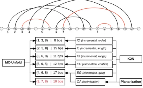
2.2 MC-Unfold is compared with the planarization and pseudoknot removal algorithms. One solution is missed (in red) by the current methods. The number of base pairs in the leftmost node of an arc indicates how many base pairs are involved. . . 18 2.3 MC-Unfold uses a divide and conquer approach to solve the

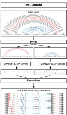
prob-lem. The subproblems are divided (red and blue). They are solved independently by a CSP solver and the full solutions are assembled back by cartesian product. . . 21 2.4 The Minizinc model used to solve the constraints is very simple

and concise. A matrix of booleans is passed to it, indicating if base pair at index i can coexist with base pair at index j. . . 22 2.5 The length and number of base pairs of the 320 tertiary structures

used to test unfolding is illustrated. The nine structures too large to unfold in reasonable time are mostly ribosomal RNAs and are identified on the right. . . 23

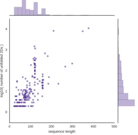
2.6 For each 3D structure which were not already planar and multiplet-free (227/320), the log10of the number of saturated 2D structure is

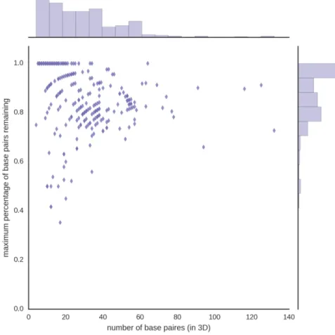
displayed against the length of the corresponding sequence, sorted by increasing length. . . 24 2.7 Some of the 218 structures completely unfolded contain large amounts

of base pairs not representable by planar multiplet-free 2D structures. 25 2.8 Some 3D structures contain significant amount of base pairs

vio-lating common constraints of 2D structure prediction algorithms (planar, multiplet-free). In general, this implies large pseudoknots (left, 2LC8) and/or multiplets (right, 4PLX). The number of base pairs is displayed next to the 2D structures. . . 26 3.1 Meta-Annotate calls on MC-Annotate, 3DNA and RNAview and

compares their results to create a high quality annotation. . . 30 3.2 The annotations of Meta-Annotate can be viewed using Chimera

along with VARNA. The canonical (blue) and non-canonical (red) base pairs of the lysine riboswitch (4ERJ) are depicted. . . 31 3.3 The PDB is filtered to keep single model and single chain RNA

monomers. . . 32 3.4 The experimental structures are compared on three levels. The

first contains all base pairs (3Dfull ), the second contains only

canonical base pairs (3Dcanonical ) and the last is all the planar

secondary structures obtained from the second one by using MC-Unfold (2Dunfolded ). . . 33

3.5 The base pair distance is the cardinality of the symmetric differ-ence between the two sets of base pairs compared. For example, given bpset1 = {(0, 6), (3, 5)} and bpset2= {(0, 6), (1, 5)}, their

symmetric difference would be {(1, 5), (3, 5)} which means a base pair set distance of two. . . 36

3.6 The distances between computational (C1-C3) and experimental (E1-E3) structures are used to find, for every computational struc-ture, the most similar experimental structure. These couples of structures are used to calculate the gap between computational and experimental structures. . . 37 3.7 The linear correlation between the minimum base pair set distance

(error) and the sequence length is shown on the set of planar (left) and non-planar (right, in grey) experimental structures. A distance of zero indicates that a computational structure matched perfectly an experimental structure. The vertical line is set at 0 or at the largest sequence with a distance of zero. ∆ is the slope, S is the standard error and R2the r squared value. . . 38 3.8 On each row, the linear correlation between the median base pair

set distance (error) and the sequence length are displayed. The 3D structure without multiplets or pseudoknots (on the left) are separated from those containing them (on the right). ∆ is the slope, S is the standard error and R2the r squared value. . . 39 3.9 The experimental structures were mostly determined by solution

NMR structures and x-ray diffraction. NMR files generally con-tain many conformers. . . 41 3.10 For each sequence length, the number of unique sequences (above)

and the total number models associated with them (below) are shown. The sequences are mostly short. . . 42 3.11 The size of clusters produced by CD-HIT-EST are counted. A

cluster size of 1 means that there was a single sequence in a cluster. 43 3.12 On the 2Dunfolded , most of the algorithms can find at least one

ex-perimental structure, some even for relatively large exex-perimental structures. . . 45 3.13 On the 2Dunfolded , the median error remains quite good. . . 46

I.1 The same sequence can be found in many different deposited PDB files. . . xiii I.2 The structures contain mostly canonical interactions. . . xiv I.3 The conformers of NMR ensembles can contain very different

base pairs. . . xv I.4 On the 3Dcanonical , non-planar structures can sometimes be

pre-dicted by methods allowing for pseudoknots. . . xvi I.5 The median error on the 3Dcanonicalis slightly higher for the

non-planar structures compared to the 2Dunfolded. . . xvii

I.6 On the 3Dfull , few of the non-planar structures can be predicted.

The minimum error is also the largest of all representations. . . . xix I.7 On the 3Dfull , the median error is the largest compared to both of

LIST OF APPENDICES

LIST OF ABBREVIATIONS

MFE Minimum Free Energy mRNA Messenger RNA

NMR Nuclear Magnetic Resonance RNA Ribonucleic Acid

2D RNA Secondary Structure 3D RNA Tertiary Structure H-bond Hydrogen Bond

MCC Matthews Correlation Coefficient CSP Constraint Satisfaction Problem PDB Protein Data Bank

CHAPTER 1

INTRODUCTION

Our knowledge of RNA started with messenger RNAs, carriers of genetic information used in protein synthesis [1]. As the years went by, RNA was found to be implicated in much more varied group of functions than was initially supposed. Currently, we know that it play essential roles in biological functions such as transcription, replication, gene silencing and even direct enzymatic activities [2, 3].

RNA molecules form highly intricate three-dimensional structures by folding back on themselves, sometimes while interacting with other molecules. A single RNA molecule has the capacity to co-exist in different structural states as well as the capacity to change structure [4–6]. These properties are crucial to its functions, for example when acting as molecular sensors and effectors [3].

Characterizing RNA structure and understanding its behavior is an important subject in biology and bio-informatics. Being able to create molecular structures can open the door to radical advances in biological engineering, medicine and industry [7].

The purpose of this chapter is to define concepts used throughout this work. We start by presenting the many models used for representing RNA and its structure. The models are organized into primary, secondary and tertiary structure, by increasing amount of infor-mation. These models are frequently used to represent experimentally determined RNA structures. Using one of the many techniques available today, constraints can be found and used to create low and high-resolution structural models. In the case of RNA, the most relevant are nuclear magnetic resonance (NMR) and X-ray crystallography. The last concept presented is the prediction of RNA structures using computational meth-ods. We are particularly interested in single-sequence secondary structure prediction, but comparative methods are also presented.

1.1 RNA Structure Models

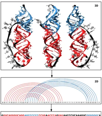
The study of RNA structure is divided into a hierarchical organization of models called structures shown in figure 1.1.

Figure 1.1: Hierarchy of structural models for RNA (pdb id:2LC8, chain A). The nu-cleotides are colored to match between the models.

The models are organized by increasing amount of information from primary to tertiary structure. The primary structure is the sequence, the string of ribonucleotides obtained by traversal of the phosphate backbone from 5’ to 3’ of the ribose. The secondary struc-ture is formed by base pairs, edge-to-edge hydrogen bonds between nucleobases. The tertiary structure is formed from interactions of secondary structure features. This work is mainly concerned with the relationship between secondary and tertiary structures, these are therefore the ones that should be well formalized before proceeding further.

1.1.1 Ribonucleotides And Primary Structure

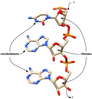
Ribonucleotides are the building blocks of RNA molecules. They can be decomposed into a nucleobase and a sugar (ribose). The nucleobases (adenine (A), cytosine (C) and guanine (G)) are shared with DNA while thymine (T) is replaced by uracil (U) in ribonucleotides. The ribose is very similar to the desoxy-ribose which forms DNA. It contains an added hydroxil group which increases its reactivity.

Figure 1.2: RNA forms a linear polymer ribonucleotides.

The primary structure S of an RNA is the sequence of ribonucleotides s1..sn, following

the phosphate backbone and ordered by the nucleotides chemical 5’ to 3’. The four most common symbols used to represent nucleotides are {A,C, G,U }, referring to the bases adenine (A), cytosine (C), guanine (G) and uracil (U) [8]. The actual number of valid nucleotide symbols is above 100 when enzymatically modified nucleotides are accounted for. They are present in some of the most well-known experimentally resolved structures such as transfer RNAs [9] and 5S ribosomal RNA [10]. Their distribution varies greatly depending on the organism and underlying function of the RNA.

1.1.2 Base Pairs And Secondary Structures

Base pairs are edge-to-edge hydrogen bonding interactions between nucleobases [11]. The canonical base pairs are the Watson-Crick base pairs A·U and C·G and the wob-ble pair G·U. They are thought of as the most stable and important ones in an RNA structure because they allow for the most amount of hydrogen bonding. Other base pairs are referred to as non-canonical. Those interactions are common in experimen-tally resolved structures, especially when accounting for modified base pairs. Base pairs are usually described by a nomenclature. Currently, the most pervasive is the Leontis-Westhof nomenclature [11]. The other notable ones are Saenger group’s [12], Guttell group’s [13] and Major group’s [14].

A secondary structure S on RNA sequence s1, ..., sn is a set of interactions between

nucleotides in the sequence s1..sn. A pair (i, j) such that i < j is used to represent an

interaction between nucleotides at index i and j in the sequence. Because of the poten-tial complexity of base-pairing patterns, many restricted and convenient definitions of secondary structure have been designed. These definitions are discussed in great details in section 2.2.2.

Illustrating secondary structure is an important task. Throughout this work, secondary structures are represented using strings in dot-bracket notation and arc-annotated draw-ings. In the dot-bracket notation [15], the dots represent unpaired positions. Opening and closing brackets are matched to indicate the first and second base in a base pair. A simple example could be the following string ”(.).” on the sequence ACUG. This would be interpreted as A pairing (opening bracket) with U (closing bracket). Dot-bracket no-tation requires the secondary structure to be planar. Non-planar features such as crossing arcs shown in red in figure 1.3 cannot be represented unambiguously with the basic no-tation [16]. The use of an extended nono-tation allowing symbols such as { } or [ ] can be used to represent non-nested base pairs unambiguously.

Figure 1.3: Secondary structure (2D) of 2LC8 chain A (PDB) depicted using VARNA. The colors correspond to those in the 3D structure of figure 1.1.

In an arc-annotated drawing, interactions between nucleotides are represented by an arc going from one to the other on the linear sequence. The advantage is that it can rep-resent tertiary structure features such as multiplets, which is not the case for dot-bracket notation, even with extended notation. An example is shown in figure 1.3, realized using VARNA [17].

There are many other useful representations for RNA secondary structure. The curious reader can consult the excellent reviews by Ponty [18] and Schirmer [19].

1.1.3 Tertiary Structure

The tertiary structure is the most detailed structural model of RNA. It represents the bi-ologically active/relevant features by their position in a three-dimensional space ((x, y, z) coordinate system). The models vary from all-atom representations to coarse descriptors An example 3D model is illustrated in cartoon-like representation in figure 1.4.

There is a myriad of tertiary motifs that have been observed in experimentally deter-mined 3D models [20]. Since the goal of this thesis is to create a correspondence be-tween base pairs in tertiary and secondary structure, the main interactions we care about are the pseudoknots and the base pairs multiplets.

Figure 1.4: Tertiary structure (3D) depiction of 2LC8 chain A (PDB).

Pseudoknots are non-nested base pairs often classified as elements of tertiary structure. They are part of tertiary structure mainly because common algorithms for secondary structures have issues dealing with the added complexity they bring [8]. They are evolu-tionarily conserved and critical to the activity of many biological molecules such as the self-splicing group I introns, E. coli’s 16S ribosomal RNA [21].

Multiplets are base pairs forming between more than two nucleobases (triplets, quadru-plets, etc...). They are mostly described as tertiary structure, but like pseudoknots, there have been attempts at representing and predicting them such as RNAWolf [22].

Although pseudoknots and multiplets are the main focus of this work, there are many other interesting features of tertiary structure worth noting such as coaxial stacking, loop-loop interactions and many others [20].

1.2 Experimental Techniques For RNA Structure Determination

This section is aimed at clarifying how experimental information is generated. Most of the 3D structural models used later were created using high-resolution methods such as crystallography and nuclear magnetic resonance spectroscopy. Acquiring structural information and building models of RNA structure is a hard task. It involves costly experiments and tricky interpretation.

Many valid techniques are left out. For a more thorough review of experimental deter-mination of RNA structure, I recommend Felden’s 2007 review [23].

1.2.1 X-ray Crystallography

X-ray crystallography is the current gold standard in high-resolution RNA structure de-termination. The process of crystallography can be separated into four steps. First, the molecules are crystallized. X-rays are then projected on them and the pattern of inter-action is captured. This pattern is used to build an electron density map, identifying regions where atoms are located. Using computer algorithms and knowledge about ge-ometry and bond lengths, models are built that fit the density map.

The crystallography of RNA is hard. The main challenge is to obtain high quality crys-tals that can diffract to atomic resolution. Crystallographers try different variations of experimental conditions (solution, temperature, additives) in order to obtain sufficient amounts of high-quality crystals [24]. In the event that there isn’t any condition that works, the sequence can be changed to improve crystallization.

A very important challenge for crystallography happens at the modeling step. The issue is that at medium and lower resolutions (more than 2.5 to 3.5 angstroms, 0.25 to 0.35 nanometer), the constraints derived from the density map are not restrictive enough. Building a model becomes error prone because the density map could accommodate many different 3D models (the system is underdetermined). There are a few tools avail-able to verify and quantify potential problems with RNA 3D models such as MolProbity

[25]. However, there are still instances of entirely incorrect structures [25, 26]. There-fore, the interpretation of crystallographic data should be done with great care.

1.2.2 Nuclear Magnetic Resonance Spectroscopy

Nuclear Magnetic Resonance spectroscopy (NMR) of RNA is another high-resolution method. It exploits the nuclear magnetic resonance effect to detect hydrogen bonding between nucleobases. With this information and auxiliary experiments, it can produce high-resolution models of 3D RNA structures [27, 28]

NMR has some advantages over other high-resolution methods. The most obvious is that it can be used to directly infer base pairing patterns. It can also be used to observe RNA dynamics and structural interchanges [29]. Being able to investigate dynamics is a significant advantage over crystallography.

NMR spectroscopy of RNA is technically challenging. RNA is made of only four nu-cleotides, which makes the resonance assignment much harder than it is for proteins. Because of this, high-resolution NMR experiments are only done on relatively small structures, compared to x-ray crystallography [28]. For more details, there is a nice review of the current approaches and their limitations [28].

1.3 RNA Secondary Structure Prediction Algorithms

Predicting the biologically relevant structure of an RNA is an extremely challenging problem. Most of the work done in structure prediction was motivated by the cost and time needed to determine structures using experimental methods. Secondary structure prediction algorithms can be separated into the comparative and statistical categories.

1.3.1 Comparative Approaches

The comparative approaches are based on the idea that functional constraints restrict the tertiary structure of a molecule. For example, a transfer RNA must adopt a cloverleaf-like structure for it to work properly. By observing patterns of homology and covariation, hypothesis can be made to drastically restrict the conformational space that needs to be explored [30, 31].

Currently, there are three approaches to comparative analysis [32]. The first is to cre-ate a sequence alignment and give it to an alignment folding algorithm such as PFold [33] or RNAAliFold[34]. The second approach is to simultaneously fold and align [35– 37]. The third is to obtain structures and assign a common structure [38].

There are many limitations to the comparative approach. Perhaps the most important is that it aims at finding a single consensus structure. Any molecule with more than a single functional structure, such as riboswitches, will elude these methods. Moreover, pseudoknots and interactions with other molecules are not modeled in most of the cur-rent approaches [32].

1.3.2 Single-Sequence Approaches

Single-sequence prediction methods are usually based on the idea that RNA secondary structure adopts the most likely structure(s) according to some statistical distribution. The main approach relies on the thermodynamic hypothesis which considers the struc-ture of minimal free energy to be biologically relevant [39].

Dynamic programming stands out as the most prominent optimization technique in single-sequence prediction algorithms. The optimization goal can be to maximizing the number of complementary base pairs [40] or minimize the free-energy in the nearest-neighbor model with experimentally-derived values [41, 42] as in MFold [43]. For more

details about how these algorithms are designed, there are excellent primers [44] and detailed accounts [8] written by dynamic programming adepts.

The limitations of current single-sequence approaches are somewhat severe. As with comparative approaches, there are many biological features which are not accounted for in common models. Most methods are restricted to canonical base pairs only and forbid pseudoknots and multiplets. Non-canonical base pairs were included into RNA secondary structure prediction in MC-Fold [45]. Pseudoknots included into rigorous free-energy minimization algorithms in a few forays such as [46]. Finally, multiple pair-ings were included in the MC-Fold-DP algorithm [22], although pseudoknots were not. The only thing that has not yet been modeled in statistical approaches is interactions with other macromolecules. An overlooked limitation of prediction algorithms based on dynamic programming is the limited precision of the parameters used to drive the optimization. Even if all assumptions of the models were satisfied, energy models such as the nearest-neighbor [42] will still suffer from experimental measurement errors. This was investigated by adding normally distributed noise well within the range of measure-ment error to free energy values of MFold. The result was that around 30 percent had different structure of minimal free energy [47].

1.4 Master’s Project

The first problem I wanted to tackle is the unfolding problem. Most 2D structure predic-tion algorithms restrict the type of base pairs and the topology of the structures predicted. For example, non-canonical base pairs, pseudoknots and multiplets are generally not al-lowed. Removing those base pairs from RNA structures is used in many applications to model, index, analyze RNA structures [48].

Currently, there are two algorithmic approaches that can remove those features from experimentally-derived structures. These are the planarization [49] and pseudoknot re-moval algorithms [48]. The main issues with those methods is that they generate one or few secondary structures while there are many possible alternatives. Moreover, they

do not handle the removal of multiplets. Since I intended to use those methods to ana-lyze experimental-derived 3D structures, I needed to extend those methods to be more exhaustive in their output and deal with multiplets. MC-Unfold was created to solve this (figure 1.5.

The other problem I was interested in is to understand how structures obtained using 2D structure prediction methods compare with those obtained using experimental methods such as NMR and X-ray crystallography. Currently, there are no evaluation that takes into account that most prediction methods predict restricted forms of secondary struc-ture. For example, if an algorithm predicts pseudoknot-free structures and the reference contains pseudoknots, we must know that the model failed, not the prediction. MC-Unfold was ideal to investigate this.

To do so, a large set of experimentally-determined 3D models of RNA was acquired from the PDB. They were verified, annotated, unfolded and associated to their respec-tive sequence to create a set of annotated 3D structures of RNA monomers. A variety of single-sequence 2D structure prediction methods were then applied on those sequences. The two sets of structures were then compared to find out if any experimental structures were contained in the predicted structures and how far on average the predictions are.

1.4.1 Structure Of The Thesis

In chapter 2, the unfolding problem is defined. The current algorithmic approaches are reviewed and analyzed to illustrate common pitfalls. A constraint programming algo-rithm named MC-Unfold is implemented along with the most common constraints of secondary structure prediction models. The code is tested and executed on a set of struc-tures previously used to evaluate RNA secondary structure prediction algorithms [50].

In chapter 3, secondary structure prediction algorithms are evaluated against a new, high-quality data set of reference structures. The construction of the data set, from PDB filtration to cleaning and base pair annotations are detailed.

CHAPTER 2

2.1 Overview

RNA secondary structure (2D) models are widely used to model, index, analyze and predict base pairing interactions in three-dimensional RNA structures (3D). In practice, 2D models are constrained so that a single 2D structure often cannot represent all base pairs present in a 3D structure.

I define the unfolding problem as the task of removing tertiary interactions (base pairs) from a 3D structure such that the resulting set(s) of base pairs respect the constraints of an RNA 2D structure. This problem is already encountered in many important applica-tions [48]. It is an essential step in predicting [51], comparing [52, 53], classifying [54] and building repositories of 2D structure such as RNAStrand [55].

Unfolding tertiary structures used to be done manually. It was relatively unreliable and non-reproducible [48]. More recently, planarization and pseudoknot removal algorithms capable of solving parts of the unfolding problem were developed [48, 49]. These al-gorithms remove base pairs with respect to some arbitrary optimization goal. The goal can be to keep the maximal amount of base pairs [49] or to find the structure of minimal free energy of a thermodynamic model [49, 56]. All the secondary structures generated are saturated, in the sense that none of the base pairs removed (e.g. part of a multiplet) could be added back without violating the constraints of 2D structure [48, 57]. These algorithmic approaches solve the previous issues of transparency and reproducibility. However, there is still place for some improvement.

The planarization and pseudoknot removal algorithms do not remove multiplets and cannot generate all saturated structures. Multiplets are not currently handled and have to be removed manually. This is problematic since it creates the same problems of non-reproducibility that motivates the existence of the methods. Moreover, interesting 2D structures can be missed because the algorithms are aimed at finding one or very few saturated structures. Since none of these structures can represent all the base pairs present in the original feature, an exhaustive method is preferred.

MC-Unfold was designed to address those issues. It is the first algorithm that can un-fold 3D structures exhaustively and handle removing pseudoknots and multiplets. MC-Unfold is based on a divide and conquer strategy and relies on a constraint satisfaction problem (CSP) solver. Despite its higher time complexity, it is capable of efficiently unfolding all but very large 3D structures (more than 400 nucleotides).

In this chapter, the previous unfolding methods [48, 49] and the tertiary interactions they can remove are detailed. MC-Unfold is then described along some implementation de-tails, including its divide and conquer strategy and its interface with the CSP solver. The applicability of MC-Unfold is then demonstrated on a large data set of annotated 3D structures from the Protein Data Bank (PDB, [58]) who were previously used to evaluate RNA 2D structure [50].

2.2 Methods

To understand well the need for MC-Unfold, section 2.2.1 describes in details the pre-vious approaches to solving similar problems (planarization, pseudoknot removal). A review of the common 2D structure constraints and the strategies used to address them is presented in section 2.2.2. MC-Unfold’s divide and conquer strategy is detailed in section 2.2.3 along with some implementation details.

2.2.1 Overview Of The Current Unfolding Algorithms

The planarization problem was proposed by Yann Ponty as part of his PhD thesis in 2008 [49]. The goal was to create a planar 2D structure with an optimality goal in mind. The first goal was to maximize the number of canonical base pairs and the second was to miminize the free energy following the Turner model (as used in Mfold [43]). A modi-fied version of the Nussinov algorithm [59] was used to solve the problem.

The pseudoknot removal problem and heuristics to solve it were proposed as part of the Knotted To Nested (K2N) package [48]. Of the six approaches, five are heuristic methods (EC, EG, IL, IO, IR) and the sixth is a generic optimization procedure which can be used to create more complex scoring schemes. The K2N framework is the one mostly in use today in applications such as the RNA Strand database [55], RNAPdbee [60], RNAStructure [61] and many others.

Saturated 2D structures are the goal of all current unfolding algorithms [48] as well as MC-Unfold. This saturation constraint states that no base pair can be added back to the unfolded structures without violating the definition of 2D structure [62]. This is crucial to avoid removing more base pairs than is absolutely necessary.

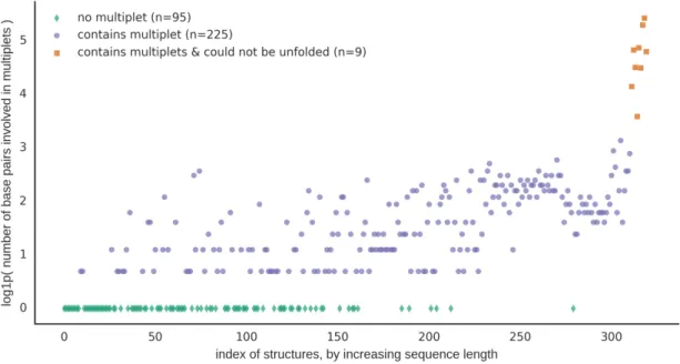
Current algorithms do not remove multiplets. Triplets and larger multiplets are not allowed in the input. Rather, they have to be dealt with manually, which creates the same problem the methods were designed to solve. Unfortunately, multiplets are common in 3D structures and that severely limits the applicability of the algorithms. Of the 320 annotated 3D structures used to test the performance of MC-Unfold (section 2.3.1, show in figure 2.1), slightly more than 70 percent (225/320) contained at least one multiplet. This is a reasonable data set that was previously used to evaluate 2D structure prediction algorithm [50]. This demonstrates that removing multiplets is a relevant issue to address.

Figure 2.1: Most of the 3D structures of the CompaRNA data set contain at least one multiplet. log1p(x)=ln(x+1)

Current methods can miss important 2D structures. Many structures can be ignored by current methods because they are not optimal according to the criteria considered. An example previously used to show the diversity of the six pseudoknot removal meth-ods illustrates this well (figure 1 of [48]). Although the six methmeth-ods are different, they sometimes return the same solution and can miss some (see figure 2.2).

Figure 2.2: MC-Unfold is compared with the planarization and pseudoknot removal algorithms. One solution is missed (in red) by the current methods. The number of base pairs in the leftmost node of an arc indicates how many base pairs are involved.

In practice, finding the saturated 2D structure with the largest amount of base pairs could lead us to ignore other relevant solutions. For example, a given 3D structure could contain two large stems forming a pseudoknot. The largest of the two stems would be the best solution and the user wouldn’t know about the other stem, which might be significant. MC-Unfold can identify 3D structures which would cause such problems to current methods (see figure 2.8). Depending on why we want to unfold a 3D structure, we might not be able to tell relevant structures from other saturated structures. In those cases, an exhaustive approach is advantageous.

2.2.2 Constraints For 2D Structure

The constraints of RNA 2D structure models are intended to allow for more efficient algorithms. For example, dynamic programming algorithms for free-energy minimiza-tion of pseudoknot-free 2D structures can find optimal soluminimiza-tion(s) in polynomial time. When pseudoknots are included, the task can be NP-complete [63], depending on the restrictions used. These constraints are therefore very useful.

The distinction is made between simple and complex constraints. Complex constraints must be dealt with by constraint solving. They implicate choices between many base pairs and multiple alternatives must be considered. Simple constraints are defined as having only one unambiguous solution. For example, given a list of base pairs, the non-canonical base pairs can be removed by filtering them out.

Complex constraints are that there should not be any pseudoknots nor multiplets in the 2D structures, to make them planar. A planar 2D structure Splanaris a 2D structure

that can be drawn on a plane without any crossing edges. Given a list of base pairs, a 2D structure is planar if there are no two base pairs (i, j), (x, y) ∈ Splanar such that

i< x < j < y. This implies that pseudoknots are forbidden. Most of the free-energy minimization algorithms restrict themselves to planar 2D structures. This is not because planar structures are most often observed in nature [64]. Rather, this constraint reduces greatly the search space and complexity of prediction algorithms [8, 46]. Multiplets are also forbidden. Although they are very common in experimentally resolved structures, they are usually considered tertiary structure features [8]. Some prediction algorithm include them, such as RNAWolf [22], but restrict themselves to triplets. To deal with a triplet involving base pairs (i, j), (i, k), we remove one of the two. This is as in K2N, where the base pairs were removed manually by visual inspection in PyMol [48]. The main difference is that we don’t choose either, but instead let the CSP solver find all possible solutions.

Simple constraints group together restrictions on the type of base pairs considered and a minimal distance in the sequence between bases involved in a base pair. Non-canonical base pairs are often ignored. Most common methods such as MFold consider only the canonical base pairs. That is the Watson-Crick base pairs (A-U, C-G and sometimes the wobble G-U). Non-canonical base pairs have been included to an extent into ContraFold [65] and MC-Fold [45]. A minimal distance between bases of a base pair is often spec-ified. This is intended to avoid sharp backbone turns in the predicted structures. It also defines the minimal size of hairpin loops. It is described by a positive integer d (e.g. d= 3) specifying that there should not be any base pair (i, j) such that | j − i| < d [66].

2.2.3 MC-Unfold: Unfolding As A Constraint Satisfaction Problem

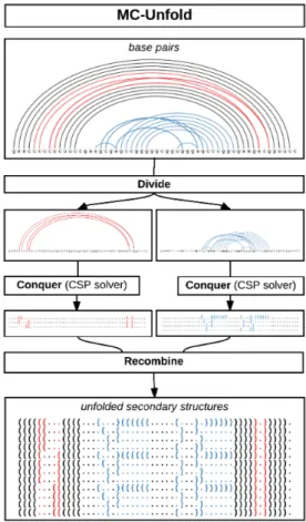
MC-Unfold uses a divide and conquer strategy (see figure 2.3). The constraints be-tween base pairs are encoded into a constraint matrix M. The value at position M[i, j] indicates that the base pairs i and j can or cannot co-exist in a 2D structure. The subprob-lems correspond to the disconnected subgraphs of the graph built from M as adjacency matrix, where an edge connects two nodes if the corresponding base pairs are conflicting.

The conquer part of the divide and conquer is solved using a CSP solver. The un-folding problem is described by a model written in Minizinc [67, 68]. This model is compiled into a set of lower-level constraints and given to a CSP solver, in this case Gecode 4.4. The CSP solvers rely on backtracking and more advanced techniques to efficiently go through the search space and find solutions satisfying the specified con-straints. The main advantages to this approach are conciseness and simplicity. The full code of the model is listed in figure 2.4.

Figure 2.3: MC-Unfold uses a divide and conquer approach to solve the problem. The subproblems are divided (red and blue). They are solved independently by a CSP solver and the full solutions are assembled back by cartesian product.

The problem solved here is hard and involves trade-offs. Given a set of base pairs S, a naive algorithms could try all possible subsets sn⊆ S and verify if snobeys all constraints

(no conflicts and saturated). This would requireO(2|S|) assuming the verification takes constant time (which is not. This is much worse than the complexity of the current unfolding methods, but as mentioned in section 2.2.1, these methods cannot yield all saturated structures. Moreover, we can apply it to almost all structures of interest as shown in sections 2.3.1 and 3.2.2.

int: n;

set of int: bp indices = 1..n;

array[1..n, 1..n] of bool: constraints; var set of bp indices: structures;

% no conflicts

constraint forall(i in structures)( forall(j in structures)(

constraints[i,j])); % saturated

constraint forall(i in (bp indices diff structures))( not ( forall(j in structures)

(constraints[i,j]) ) ); solve satisfy;

output [show(structures)];

Figure 2.4: The Minizinc model used to solve the constraints is very simple and concise. A matrix of booleans is passed to it, indicating if base pair at index i can coexist with base pair at index j.

2.3 Results

To evaluate the applicability of MC-Unfold, it was tested on a large set of 3D structures with complex base pairing topologies. MC-Unfold turns out to be very efficient and capable of completely unfolding 218 out of 227 of the 3D structures in less than five minutes on a desktop computer. The remaining nine are mostly large ribosomal RNAs.

The saturated 2D structures determined by MC-Unfold can be used to identify interesting 3D structure which do not conform well to the model of multiplet-free planar structures.

2.3.1 MC-Unfold Unfolds 3D Structures Efficiently

A data set of RNA 3D structures from the PDB was used to demonstrate the per-formance of MC-Unfold. The Protein Data Bank [58] is a repository of 3D models at atomic resolution. The models are built from high-resolution methods such as crys-tallography and NMR. This data is an interesting source of information for structural prediction, because of the resolution and the quality.

As part of the CompaRNA project, RNA 3D structures from the PDB were cleaned using modeRNA [69] and annotated using RNAVIEW [70]. The resulting data set contains a high-quality and non-redundant subset of the PDB. Problematic structures, such as the ones containing backbone breaks, less than 20 nucleotides and redundant ones were fil-tered out [50]. Modified nucleotides were replaced by unmodified nucleotide according to the mapping established in Modomics [9]. Summary statistics about the length and number of base pairs identified are displayed in figure 2.5.

Figure 2.5: The length and number of base pairs of the 320 tertiary structures used to test unfolding is illustrated. The nine structures too large to unfold in reasonable time are mostly ribosomal RNAs and are identified on the right.

MC-Unfold unfolds 3D structures efficiently. The goal of this experiment was to test MC-Unfold under realistic conditions. To do so, the full annotation (canonical and non-canonical base pairs) and all of the complex constraints detailed in section ?? were used. To summarize, MC-Unfold was used to find planar, multiplet-free saturated 2D structures without any base pair excluded.

Figure 2.6: For each 3D structure which were not already planar and multiplet-free (227/320), the log10 of the number of saturated 2D structure is displayed against the

length of the corresponding sequence, sorted by increasing length.

Out of 227 structures that were not already planar and multiplet-free, 96.9 percent (218/227) were unfolded completely while the remaining 9 could be unfolded partially, perhaps fully with better computing power. It took 207 seconds (3 mins 27) on an Intel i5-4590 CPU (3.30GHz) to completely unfold the 218 3D structures. MC-Unfold is therefore sufficiently efficient to unfold small to medium RNA 3D models.

2.3.2 2D Structures Cannot Represent All Base Pairs

Given RNA 3D structure it is interesting to know how much of the base pairs can be represented in a 2D structure model. It allows us to identify the structures which do not fit well a model of 2D structure.

Figure 2.7: Some of the 218 structures completely unfolded contain large amounts of base pairs not representable by planar multiplet-free 2D structures.

The 3D structures with highest percentage of base pairs removed tend to contain large amount of multiplets or pseudoknots, as illustrated in figure 2.8. In this case, this is caused by the particular constraints used to test MC-Unfold.

Figure 2.8: Some 3D structures contain significant amount of base pairs violating com-mon constraints of 2D structure prediction algorithms (planar, multiplet-free). In gen-eral, this implies large pseudoknots (left, 2LC8) and/or multiplets (right, 4PLX). The number of base pairs is displayed next to the 2D structures.

Structures such as those shown in figure 2.8 would be hard to predict for most 2D struc-ture prediction algorithms because they are far from planar or multiplet-free. Identifying those 3D structures comes in handy in chapter 3 to evaluate RNA 2D structure prediction algorithms. The idea is that if a 3D structure contains significant amounts of base pairs that cannot be represented in 2D structure, it should be taken into account.

2.4 Summary And Conclusion

MC-Unfold was designed to address the lack of methods capable of unfolding exhaus-tively 3D structures, including those with multiplets. A divide and conquer strategy is used to separate base pairs into independent subproblems which are solved using a CSP solver. The solutions are combined back using the cartesian product of the sets of base pairs. The implementation of the algorithm was tested on a set of annotated 3D struc-tures used to evaluate 2D structure prediction algorithm [50]. Of the 227 3D strucstruc-tures it was tested with, 218 can be fully unfolded into all their possible saturated 2D structures within less than five minutes on desktop computer. The remaining nine structures could be unfolded given more time and computing power, but the result might be too large for practical applications. Structures resulting from the unfolding process can be used to determine how well a 3D structure fit constraints of 2D structures. This is done by counting the amount of base pairs removed in the unfolded 2D structures. Identifying these structures comes in handy later when evaluating 2D structures in chapter 3.

Overall, MC-Unfold is a practical and exhaustive approach to unfolding which extends the previous planarization and pseudoknot removal algorithms with the capability of removing multiplets. Furthermore, since it finds all saturated 2D structures, it is guaran-teed to find all solutions which would have been returned by the previous algorithms. Its performance is satisfying and it is ready for practical applications.

Further works remains to be done on the unfolding problem. New constraints could enable us to extract information about more complex structures, albeit at a coarser level. One very interesting constraint which could reduce the complexity large molecules is to remove base pairs not forming helices [71]. Another interesting improvement would be to sample the space of saturated structures instead of enumerating it.

CHAPTER 3

COMPUTATIONAL VS EXPERIMENTAL STRUCTURES

3.1 Overview

RNA secondary structure prediction algorithms aim at predicting the organization of base pairs from sequence information. The idea is that RNA folding occurs in a hier-archical manner. First the sequence forms base pairs and adopts a secondary structure. Then tertiary interactions form and define the active tertiary structure [20, 72, 73]. These algorithms were developed because experimental methods are generally too costly for large scale application.

There currently exists more than 30 computational methods to predict different versions of secondary structure. Most are focused on predicting the canonical base pairs of planar secondary structures but some also pseudoknotted secondary structures [46, 74, 75] and even multiplets [22]. Obtaining the optimal pseudoknotted secondary structures accord-ing to free energie strategies is much more complex [63], but fits the observed models of secondary structures with more fidelity.

Evaluating prediction algorithms relies on correlation between different structure deter-mination methods. Previous benchmark have examined the correlation of comparative prediction algorithms against comparative structure models [32] and single-sequence predictions against NMR/Crystallography models [50].

The previous benchmarks left some interesting questions unanswered. First and fore-most, can methods predicting multiple structures find an exact experimental struc-ture? In the same line of thought, how far are most of those predicted structures from experimental structures?

To address these issues, a new benchmark was designed. First, a data set of RNA monomer 3D structures was constructed from a subset of the PDB [58]. A new method dubbed Meta-Annotate was built upon the three most popular annotation algorithms (3DNA [76], MC-Annotate [77] and RNAview [70]). It compares the annotations pro-vided by those three methods to infer a consensus annotation. These annotations were used to identify base pairs in 3D structures and build the set of experimental structures, by mapping each sequence to all of its corresponding 3D models. The set of compu-tational structures was obtained under various strategies such as suboptimal structures, stochastic samples of the suboptimal structures as well as other methods. The compu-tational and experimental structures were compared by finding for each compucompu-tational structures the closest matching ones in the experimental set. The minimum and median values for each sequence were reported and their value correlated with the length of the sequence.

3.2 Methods

The goal of this chapter is to investigate how much correlation there is between sec-ondary structure prediction algorithms and experimentally-determined 3D structures. This involves examining available experimental structures to identify their base pairs. These are then used to generate the set of experimental structures. The computational structures are then obtained by feeding the sequence of experimental structures to the secondary structure prediction methods. Finally, these computational and experimen-tal structures are compared to assess how close the computational structures are to the experimental ones.

3.2.1 Meta-Annotate Creates Consensus Annotations

Identifying base pairs in 3D models involves finding chemical group in a geometry sus-ceptible of forming hydrogen bonds between nucleobases. The general approach is to find nucleobases in close proximity and examine geometric properties to detect probable hydrogen bonding sites. MC-Annotate [14, 77] relies on Gaussian mixture models to

compute the likelihood of H-bonds between donor and acceptor chemical groups. These H-bonds probabilities define a graph on which the maximum flow algorithm is applied to model competition between donors and acceptors. H-bonds above a certain threshold are kept and base pairing types assigned depending on local geometry of the bases and hydrogen-bonds. RNAview [70] and 3DNA-DSSR [76, 78–80] use purely geometrical rules to annotate base-pairs in 3D structures. Base pairs are deduced by verifying if they satisfy certain conditions, which are mostly geometrical.

Meta-Annotate creates a consensus annotation by combining the result of other an-notation software. It compares and searches for agreement on anan-notations performed by RNAview [70], MC-Annotate (version 1.5, using mccore 1.6.2) [14, 77] and 3DNA-DSSR (version 1.6.2-2016sept19)[76, 78–80]. A base pair is considered only if a ma-jority of the annotators identifies a base pair between Watson, Hoogsteen or sugar edge of a nucleobase (see figure 3.1). It is currently limited to PDB files that contain a single chain of an RNA monomer.

Figure 3.1: Meta-Annotate calls on MC-Annotate, 3DNA and RNAview and compares their results to create a high quality annotation.

The consensus annotations can be examined visually. A small python script relying on the the Chimera molecular viewer [81] was created. It changes the default visual style and attributes color to the nucleobases depending on the type of interactions, as can be seen in figure 3.2.

Figure 3.2: The annotations of Meta-Annotate can be viewed using Chimera along with VARNA. The canonical (blue) and non-canonical (red) base pairs of the lysine riboswitch (4ERJ) are depicted.

3.2.2 Preparing Experimental Structures

The first step is to build a data set of experimental structures. Experimental struc-tures are strucstruc-tures determined by biochemical or biophysical methods (e.g. NMR, crys-tallography). The number of experimentally determined RNA structures has increase a lot in recent years. In 1995, years after most of the development of RNA secondary structure prediction strategies (e.g. mfold, etc.) were done, the PDB [58] contained only 31 available 3D structures of RNA or RNA-protein mixes. This number eventually grew to 155 in 2005 and then 462 in 2015 [82].

A new data set of annotated experimental structures was prepared from the PDB database. The data set used in CompaRNA was an interesting candidate, but contained large amounts of non-monomers and the annotation was based solely on RNAview. To

improved upon this, we used a subset of RNA models from the PDB and annotated them using Meta-Annotate. A large amount of 3D models were filtered out. Only 3D mod-els of RNA monomers are considered. These modmod-els must not be in association with proteins or DNA molecules or contain modified nucleotides. The filtration process is il-lustrated in figure 3.3. Of the 4857 unique 3D models obtained from the PDB, 4223 (87 percent) were successfully cleaned and annotated. Models filtered out contained mod-ified nucleotides and abnormalities which the annotation software could not deal with. Moreover, molecules of more than 1000 nucleotides (pdb ids 3J28, 3J2A, 3J2B, 3J2D, 3J2E, 3J2F, 3J2G, 3J2H) were removed to avoid performance issues with MC-Unfold as well as the structure prediction algorithms.

Figure 3.3: The PDB is filtered to keep single model and single chain RNA monomers.

There are often many 3D models representing the same sequence. For example, NMR structures often contain many conformers [27] while crystallographic structures may contain the same RNA interacting with a different ligand. Since all these structures have been observed, the sequence is mapped to all potential structures and they all are valid experimental structures.

Three versions of the consensus annotations are considered, that is 3Dfull, 3Dcanonical

and 2Dunfolded (see figure 3.4). The 3Dfull contain all the base pairs present in the

con-sensus annotation. including non-canonical base pairs. This is intended to give an honest appraisal of how well the computational structures match all the known base pairs. The 3Dcanonicalis the set of canonical base pairs in the 3D models. This is intended to give an

con-tribute most to the stabilization of 3D structures. The 2Dunfolded is the set of all unfolded

secondary structures created by MC-Unfold on the 3Dcanonical. The constraints used are

that there is no multiplet nor non-planar base pairs. This should be the most reasonable version of 3D structures, since it conforms many of the underlying assumptions used in computational methods.

Figure 3.4: The experimental structures are compared on three levels. The first contains all base pairs (3Dfull ), the second contains only canonical base pairs (3Dcanonical) and

the last is all the planar secondary structures obtained from the second one by using MC-Unfold (2Dunfolded ).

Experimental structures are separated into planar and non-planar structures. This is done on the basis of them containing non-planar base pairs and/or multiplets, as was done in CompaRNA [50]. The planar structures should be the easiest to predict since they fit the models used in planar secondary prediction algorithms (CentroidFold, RNA-subopt, RNAstructure, SFold). The non-planar structures can still be predicted by the methods allowing for pseudoknots (HotKnots, IPknot), as long as there are no multiplets or non-conical base pairs involved.

3.2.3 Preparing Computational Structures

The second step is to acquire computational structures. Computational structures are structures predicted by a folding algorithm. Computational methods used range from statistical sampling (SFold, RNAstructure’s stochastic, RNAsubopt) to the prediction of suboptimal structures at an energy range above the MFE (RNAsubopt, RNAstructure’s AllSub) and others (CentroidFold, IPknot and Hotknots). The prediction methods tested can be separated into three groups. The first type is the generation of suboptimal sec-ondary structures. The second is the generation of a sample of secsec-ondary structures from the Boltzmann ensemble. The last group contains methods based on generalized centroid estimators and heuristic approaches to predict pseudoknotted structures.

The first group of methods general of suboptimal structures within an energy range above the MFE. This technique that was devised to address issues with the prediction of secondary structure by minimal free energy [83, 84]. Inconsistencies with the nearest-neighbor model, the possibility of structures at non-equilibrium and the existence of molecules existing in many states such as riboswitches motivated researchers to inves-tigate more structures of high probability. For each sequence, a set of at most 100 sub-optimal structures was considered. In many instances, the sequences were small enough that there was much less than 100 considered. The two methods for suboptimal structure prediction are RNAStructure (AllSub version 5.8.1), from the RNAstructure package [61] and RNAsubopt (version 2.2.10) from the Vienna package [85].

The second group of methods perform the proportional sampling of suboptimal structures according to their probability of existence in the thermodynamic ensemble (following a Boltzmann distribution) [84]. The resulting ensemble is often clustered to reveal representative structures. The full set of secondary structures, not the repre-sentative structures is used to compare them to experimental structures. By default, a

especially for small sequences. The three methods that use stochastic ensemble are RNAstructure-stoch (stochastic, version 5.8.1) from the RNAstructure package [61], RNAsubopt-stoch (RNAsubopt using –stochBT option, version 2.2.10) from the Vi-enna package and SFold-stoch (SFold, version 2.2-20110126) [86, 87].

The third group of approaches rely on γ-centroid estimators, integer programming and other heuristics. CentroidFold (version 0.0.15) predicts secondary structures us-ing γ-centroid estimators [88]. This corresponds to optimizus-ing an objective function which is the weighted sum of the expected number of true positives and true negatives base pairs. The γ parameter adjusts the sensitivity and positive predictive value of the proposed secondary structures. Values of gamma in the range of 2−5 to 210 were used by setting the gamma option to -1. This allows us to observe the effects of gamma on structures generated. IPknot (version 0.0.4) is an extension of CentroidFold that can predict pseudoknotted structures [74] using integer programming. The default settings were used. HotKnots (version 2.0) is an heuristic method for the prediction of secondary structures with pseudoknots. Stems of high stability are iteratively formed and added to substructures until none are left to be added. Hotknots was used with default parameters.

3.2.4 Comparing Experimental And Computational Structures

The last step of the evaluation is to create a method to measure how similar compu-tational and experimental structures are. To do so, we need to represent what we care about when we compare two RNA structures. A distance function d is a function that maps a pair of objects to a non-negative real numbers (d : X × X → [0, ∞)) and satisfies the following three conditions.

1. d(x, y) = d(y, x) (symmetry)

2. d(x, y) = 0 ↔ x = y (identity of indiscernibles) 3. d(x, z) ≤ d(x, y) + d(y, z) (triangle inequality)

The base pair set distance is a simple distance function which is used on sets of base pairs. It is applicable on sets of base pairs without restrictions which means we can use it to compare structures containing non-planar and multiplets. Its value is the cardinality of the symmetric difference of the two set of base pairs representing the structures com-pared. A distance of N means that there are N base pairs that are not in the intersection of the two base pair sets [19]. Its minimum value is zero and its maximum can go up to the size of the union of the two sets (|bpset1| + |bpset2|) if the intersection is empty.

Although the base pair set distance is not applicable to all situations, it applies well here because we compare structures belonging to the same sequence. This means that they have the same length and each nucleotide corresponds one-to-one between the structures [19].

def base pair set distance(bpset1: set, bpset2: set) −> int: sym diff = bpset1.symmetric difference(bpset2)

return len(sym diff)

Figure 3.5: The base pair distance is the cardinality of the symmetric difference be-tween the two sets of base pairs compared. For example, given bpset1 = {(0, 6), (3, 5)}

and bpset2= {(0, 6), (1, 5)}, their symmetric difference would be {(1, 5), (3, 5)} which

means a base pair set distance of two.

Since many sequences have more than one experimental structure, each computational structure is paired with its most similar experimental structure. This is the structure which minimizes the base pair set distance. This process is illustrated in figure 3.6. Once the computational structures are paired with their most similar experimental structure, we can evaluate how close the predictions are. The sequence length is correlated with the minimum or median base pair distances of those pairs of structures using linear regression. The minimum and median errors are correlated with the sequence length be-cause it is available to the user and can be linked to the number of possible structures [16]. This analysis is not intended to generalize outside of the structures tested but in-stead is a way of summarizing the results. Goodness of fit tests are performed on the

Figure 3.6: The distances between computational (C1-C3) and experimental (E1-E3) structures are used to find, for every computational structure, the most similar exper-imental structure. These couples of structures are used to calculate the gap between computational and experimental structures.

linear regressions. Two measures used are the coefficient of determination and the stan-dard error of the estimate. The coefficient of determination, or R squared, adopts values are between 0 and 1, where a larger value indicates a better match between regression performance. The standard error of the estimate is the square root of the average squared deviation. Values near zero indicate better fit.

How Close Are The Best Predictions? The minimum error test was designed to find out if it is possible to find any of the experimental structure in the set of computational structures. For each sequence, we select the computational structure which had the least difference with an experimental structure (closest to zero). We call this the prediction of minimum error. A distance of zero implies that one of the computational structures is contained within the corresponding experimental structures. Although it happens some-times, it is common that the computational methods will not predict exactly any of the experimental structures. This might be attributed to the presence of features that could not have been represented in the secondary structure model (pseudoknots, multiplets) or prediction errors.

Figure 3.7: The linear correlation between the minimum base pair set distance (error) and the sequence length is shown on the set of planar (left) and non-planar (right, in grey) experimental structures. A distance of zero indicates that a computational structure matched perfectly an experimental structure. The vertical line is set at 0 or at the largest sequence with a distance of zero. ∆ is the slope, S is the standard error and R2 the r squared value.

The minimum error values must not be used to compare computational methods be-tween themselves, but instead to compare them with the experimental structures. For example, methods based on stochastic samples of the suboptimals will usually performs best in this test because the set of predicted is larger and more varied than for other methods. The median error calculated in the next test is a better indicator of relative performance.

Another important aspect of this analysis is that even though the distances shown in fig-ure 3.7 may appear relatively benign, small sequences usually contain only a few base pairs. Therefore, a large percentage of base pairs predicted can be wrong while the over-all distance remains smover-all.

How Close Are The Overall Predictions? The median test measures the central ten-dency of the distance between computational and experimental structures. A large me-dian value indicates that the computational and experimental structures are dissimilar. The median is preferred to the mean for its robustness to outliers, meaning it wouldn’t be affected by a few extremely large or small distance values.

Figure 3.8: On each row, the linear correlation between the median base pair set distance (error) and the sequence length are displayed. The 3D structure without multiplets or pseudoknots (on the left) are separated from those containing them (on the right). ∆ is the slope, S is the standard error and R2the r squared value.

The median test can be used to model how well a predicted structure would fit if it was picked at random amongst the set of predicted structures. It is less affected by different amounts of predicted structures than the minimum error test. As such, it can be used to compare computational methods between themselves.

3.3 Results

Th set of experimental structures is first described. To our knowledge, this is the first and largest data set of annotated single-chain RNA structures, without any modified base pairs, solely from experimental sources. The comparison of computational and experi-mental structures is presented in section 3.3.2. Computational structures are compared with the 2Dunfolded set of experimental structures described in section 3.2.2. The

re-sults are encouraging and useful to understand the extent and limitations of the current single-sequence secondary structure algorithms.

3.3.1 A New High Quality Set Of Reference Structures

With over 4223 models accounting for 321 sequences, the collection of annotated struc-tures done here is the largest collection of single chain RNA strucstruc-tures containing no modified nucleotides.

Overall, the experimental structures are mostly small (below 50 nucleotides) determined by NMR and X-Ray crystallography. Although the 3D models contain no modified nu-cleotides nor intermolecular interactions with proteins, a few structures contain ligands.

There is variety in sequence (both length and similarity), the type of experimental tech-niques used and the variety of RNA structures they present (types of base pairs, distance between models of the same sequence). All of the information related to the PDB struc-tures was acquired using PyPDB to query the PDB [89].

3.3.1.1 The Models Are Mostly From NMR and X-Ray Crystallography Most of the experimental structures were determined by NMR and crystallography.

Figure 3.9: The experimental structures were mostly determined by solution NMR struc-tures and x-ray diffraction. NMR files generally contain many conformers.

In figure 3.9, we can see that most of the PDB ids identified originate from NMR and crystallography. This however doesn’t take into account that the files deposited with a single PDB may contain many 3D structures for the same sequence. The number of 3D models, determined by NMR is therefore much higher than suggested by counting the files.

3.3.1.2 The Sequences And Models Are Small

There is a total of 321 unique sequences which correspond to 4223 3D models.

Figure 3.10: For each sequence length, the number of unique sequences (above) and the total number models associated with them (below) are shown. The sequences are mostly short.

In figure 3.10, we can see that most of the sequences are short. Moreover, the number of 3D model is generally greater for small sequences. This can be explained by the abundance of NMR models of small RNA sequences.

3.3.1.3 The Sequences Are Diverse

For the evaluation to be relevant, the RNA sequences should be varied. To make sure that the sequences have some variation, the sequences were clustered using CD-HIT-EST at a cut-off value of 0.9 sequence identity [90].

Figure 3.11: The size of clusters produced by CD-HIT-EST are counted. A cluster size of 1 means that there was a single sequence in a cluster.

Most of the cluster sizes are small (see fig 3.11), indicating that the sequences are varied. There are some larger clusters, which come from well-known molecules such as the U6 internal stem loop, the tetrahydrofolate riboswitch and the HIV Tar loop.