HAL Id: hal-01709492
https://hal.archives-ouvertes.fr/hal-01709492
Submitted on 15 Feb 2019
HAL is a multi-disciplinary open access
archive for the deposit and dissemination of
sci-entific research documents, whether they are
pub-lished or not. The documents may come from
teaching and research institutions in France or
abroad, or from public or private research centers.
L’archive ouverte pluridisciplinaire HAL, est
destinée au dépôt et à la diffusion de documents
scientifiques de niveau recherche, publiés ou non,
émanant des établissements d’enseignement et de
recherche français ou étrangers, des laboratoires
publics ou privés.
Infrared heating stage simulation of semi-transparent
media (PET) using ray tracing method
Benoit Cosson, Fabrice Schmidt, Yannick Le Maoult, Maxime Bordival
To cite this version:
Benoit Cosson, Fabrice Schmidt, Yannick Le Maoult, Maxime Bordival. Infrared heating stage
simu-lation of semi-transparent media (PET) using ray tracing method. International Journal of Material
Forming, Springer Verlag, 2011, 4 (1), pp.1-10. �10.1007/s12289-010-0985-8�. �hal-01709492�
Infrared heating stage simulation of semi-transparent
media (PET) using ray tracing method
Benoit Cosson · Fabrice Schmidt · Yannick Le Maoult · Maxime Bordival
Abstract Stretch blow molding or thermoforming processes includes an infrared heating stage of the thermoplastic preform by infrared heaters. The knowl-edge of the temperature distribution on the surface and through the thickness of the preform is important to make good prediction of thickness and properties of the manufactured parts. Currently in industry, the fitting of the process parameters is given by experience and is expensive. Our objective is to provide tools that are able to simulate the heat transfers between infrared heaters and preforms in order to reduce the fitting cost and to control the qualities of the end products. The optical method called “ray tracing” is used to simulate the radiative transfer. First, we compare the ray tracing method with the view factor method on a simple example: the heating of a square sheet by one infrared lamp. Then, we perform 3D heating stage simulations and compare with experiments. The ray tracing method allows to compute a source term in the transient heat balance equation. Then commercial finite element method softwares can be used to solve the heat balance equation.
Keywords Infrared heating · Ray tracing ·
Stretch blow molding · Thermoforming processes · Semi-transparent media · PET
B. Cosson (
B
)TCPIM, Ecole des Mines de Douai, 941 Rue C. Bourseul, BP 10838, 59508, Douai Cedex, France
e-mail: [email protected]
F. Schmidt · Y. Le Maoult · M. Bordival CROMeP, Université de Toulouse, Mines Albi, Campus Jarlard, 81013 Albi, Cedex 09, France
Introduction
The beverage market is a worldwide market. A great part of bottles used for the packaging are produced using the process of injection stretch-blow molding. For example only one industrial blower can produce up to 50,000 bottles per hour. So, the number of bottles produced per day, for only one machine, is around 1.2 million. This process is a two-step process. The first one is the injection of a preform and the second one, that can be performed in another place, is the stretch blow molding. Before the blowing stage, preforms have to be reheated. The technical solution used to heat preform is infrared (IR) oven (made of different modules of less than ten lamps). The cost of the energy being more and more expensive, the optimization of the heating stage of preform becomes an important challenge for industry.
In this paper, we propose numerical tools in order to perform temperature calculation. In previous works [2,13] the stretch blow molding simulations were car-ried out by applying constant temperature through the thickness. But in fact, there is a temperature gradient and that makes important material property variations. Two principal methods are used is this kind of prob-lem. The first one, usually used in 3D image rendering and called view factor method, is already used in IR heating problems. This method is efficient for problem with opaque materials, where surface information is needed, but for problems with semi-transparent materi-als, the view factor method cannot provide information inside the material. In order to avoid this problem, authors [4,10] assume a normal propagation of the heat flux from the inner surface. This assumption provide good results for thin and plane parts. But, in the case of
the stretch blow molding, preforms are often thick and have cylindrical shapes. Taking into account these geo-metrical constraints, we choose the ray tracing method, that is also used in 3D image rendering. The ray tracing method is more time consuming than the view factor method, but it is close to the physical description of infrared heating problems.
The heat balance equation (Eq. 1) of the heating stage of preform by IR lamps is solved in two steps. First, we compute the radiative source term ∇.qr (Eq.
5) by using the ray tracing method. Then the results are used in a commercial finite elements software (Com-sol®) as an input data. In order to validate the proposed method, the ray tracing method is compared to the view factor method, then numerical results and experimental results [8] are confronted in two representative cases of thermoforming and stretch blow molding processes, the heating stages of a PET sheet and a cylindrical PET preform. Sheets and preforms used in this study are made with the PET T74F9 from Tergal industries. Heat transfer modeling
The temperature of the preform (sheet-shape or tube-shape) during the heating stage can be calculated by solving the following equation:
ρCpdTdt = ∇ ·(k∇
¯T) − ∇.qr (1)
where ρ, Cp, k are respectively the specific mass, the
specific heat and the thermal conductivity of PET. Cpis
assumed to be temperature-dependent: strong increase above the glass transition temperature (Tg≈ 350 K)
can be seen on Fig.1. The thermo-optical parameters
250 300 350 400 450 500 1000 1100 1200 1300 1400 1500 1600 1700 1800 Temperature (K) Specific heat (J.kg 1.K 1)
Fig. 1 PET specific heat versus temperature [13]
Table 1 Thermo-optical parameters of PET
Parameter Value Reference
ρ 1,335 kg.m−3 [6]
Cp See on Fig.1 [13]
k 0.25 W.m−1.K−1 [13]
κλ See on Fig.2 [8]
are referenced in Table 1. The radiative heat flux qr,
due to the IR lamps, is given by Eq. 2 according to the Beer-Lambert’s law (Eq.3) under the assumption of the non-scattering cold medium [7]. IR lamps are assumed to behave like isothermal grey bodies with an emissivity ε. ∇.qr(x) = − ! ∞ 0 ! S2κ λIλ(x, s)dsdλ (2) Iλ(x, s) = Iλ(x p,s)e−κλ(x−xp) (3) ∇.qr(x) = − ! ∞ 0 ! S2 κλIλ(xp,s)e−κ λ(x−x p)dsdλ (4) ∇.qr(x) = − ! ∞ 0 κλMλ(xp)e−κ λ(x−x p)dλ (5)
κλ is the spectral absorption coefficient of PET
(Fig. 2), Mλ(x
p) is the incident spectral emissive
power (from the lamps to the preform). Mλ(x
p)
(W.m−2.µm−1) is given by the Planck’s law [7] and
represents the power received by the preform skin from the lamp. xp is the vector that represents the path of
the ray come from the lamp and arrived on the preform skin. x is the current position of the ray. So, x − xpis the
path of the ray in the preform. The tungsten emissivity εis 0.26 is an integrated coefficient and is assumed to be constant. PET radiative properties were measured
0 5 10 15 20 25 30 0 1 2 3 4 5 6 7 8x 10 4 Wavelength (µm) Absorption coefficient(m 1)
according to the protocols defined in [9]. Measurements were performed on PET T74F9 samples using a Perkin Elmer FTIR spectrometer (spectrum 2000) over the range 1–25 µm (Fig.2). It covers 80% of the spectral emission of IR lamps, for a filament temperature close to 2400 K. κλis assumed temperature independent until
the PET is crystallized.
In this study, the source term ∇.qr in Eq.5 is
com-puted by using the ray tracing method. Ray tracing method
Physical background
The ray tracing method is usually used in 3D image rendering. This method is very close to the physics of light propagation, a ray can represent the path of a photon. Ray tracing allows the simulation of a wide variety of optical effects, such as reflection, refraction and absorption. In addition, this method enables to take into account most of constitutive elements of an IR oven like multiple lamps (various geometries) and reflectors (ceramic or metallic).
In our ray tracing software, assumptions are made for the different optical properties of lamps, reflectors and preforms. Those assumptions are referenced in Table2for the following properties: emission, absorp-tion, reflection and refraction. Reflection and refrac-tion are averaged in order to reduce the number of rays stored in each calculation. In fact, for one ray that comes from the lamp and contained all the spectral information, if spectral reflection (or refraction) is com-puted, one ray by spectral band (an infinity for an exact model) has to be created for each air-PET interface crossing.
The spectral PET reflection is plotted in Fig.3. The variation of the reflectance rλ
PETin the 0.2–20 µm
spec-tral band is between 2% and 12%. Due to this small variation, we assume a constant reflectance rPET and
we take the mean value in the spectral band 0.2–20 µm (rPET= 7%). The PET refractive index nPET (Fig. 4)
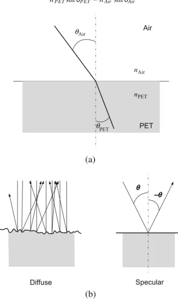
is computed by Eq.6 that gives the relation between reflection and refraction. The calculated value of the refractive index is taken equal to 1.7. The direction change of a ray that crosses a PET-air interface is given
Mean value = 7% Wavelength (µm) Reflexion (%) 0 2 4 6 8 10 12 14 16 18 14 12 10 8 6 4 2 0
Fig. 3 Spectral reflection rλof PET [8]
by the Snell-Descartes law (Eq.7), where nAir(= 1) is
the refractive index of air.
rPET=(nPET− 1) 2
(nPET+ 1)2 (6)
nPETsin θPET= nAirsin θAir (7)
Optical properties of metallic and ceramic reflectors are given in [8]. The metallic reflector reflectance rMR
is around 80% and depend of the state of conservation of the reflector: corrosion, cleanliness. The ceramic reflector reflectance cannot be easily obtained and it is computed, by inverse identification, by comparing two lamps: with and without ceramic reflector. The result of this comparison gives a global reflectance that takes into account the multiple reflections on the ceramic reflector (Fig.5). The value of this global reflectance
rCRis 35%.
In our software, only the lamp filament is taken into account. Filaments are modeled by equivalent cylin-ders, the spiral form is neglected. Tungsten filaments are assumed to be Lambertian grey bodies. This as-sumption provides the definition of ray direction vec-tors (Fig. 6) for rays coming from the filament. The direction vector −→d is defined by 2 parameters: θ ∈ [0, π/2] and φ ∈ [0, 2π]. In our first simulations, we used a discretization with constant step, as described on Fig.6b, and the results of the ray tracing software was very discretization dependent.
In order to avoid this problem, parameters θ and φ are represented by stochastic variables ( and )
Table 2 Assumptions on
optical properties Lamps EmissionSpectral and isotropic AbsorptionNone ReflectionNone RefractionNone PET Averaged Spectral Specular and averaged Averaged Ceramic reflector None Opaque Diffuse and averaged None Metallic reflector None Opaque Specular and averaged None
nPETsin PET nAir sin Air
θ
θ
(a)
(b)
Fig. 4 a Snell-Descartes law representation, b reflection types
Fig. 5 Visualization of multiple reflections in a ceramic reflector
Fig. 6 Ray definition for ray tracing
respectively. Both variables are independent and are defined by Eq.8, the use of this representation, for a Lambertian surface, is given in [11]. In the next section, the benefit of this description will be highlighted. (= arcsin("X1)
)= 2π X2 (8)
Where X1and X2are independent uniform
stochas-tic variables in the range [0; 1]. Comparison with view factor method
In order to validate our software of ray tracing, more exactly our choice of direction definition (Eq. 8), we compare its results with an analytical solution (Eq.9), given by view factor [5], in a representative case.
We choose the configuration of a squared sheet heated by one lamp (Fig. 7) of same length. This case is close to the infrared heating stage of polymer sheets used for thermoforming. The lamp is modeled by a cylinder and the sheet is the sum of infinitesimal surfaces (Fig. 8). The irradiation (W.m−2) exchanged
between lamp and sheet is computed with ray tracing and view factor respectively.
Fd1−2= PS B − S 2Bπ ⎧ ⎪ ⎪ ⎪ ⎪ ⎪ ⎪ ⎨ ⎪ ⎪ ⎪ ⎪ ⎪ ⎪ ⎩ cos'Y2−B+1 A−1 ( + cos−1'C−B+1 C+B−1 ( −Y√ A+1
(A−1)2+4Y2cos
−1'Y2−B+1 √ B(A−1) ( −√C√ C+B+1 (C+B−1)2+4Ccos −1'√C−B+1 B(C+B−1 ( +H cos−1'√1 B ( ⎫ ⎪ ⎪ ⎪ ⎪ ⎪ ⎪ ⎬ ⎪ ⎪ ⎪ ⎪ ⎪ ⎪ ⎭ (9)
Fig. 7 Geometrical configuration of the lamp and the sheet
A = X2+ Y2+ S2; B = S2+ X2; C = (H − Y)2
S = s/r ; X = x/r ; Y = y/r ; H = h/r (10) The geometrical variables (s, x, y, h) are defined on the Fig.8. The power P of the lamp is taken equal to 1,000 W.
Equation 9 gives the irradiation (W.m−2) of a
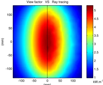
differential element of plan irradiated by a cylinder. The view factor computation is on the left side of the Fig.9 for the conditions described in Fig.7. The right side of Fig. 9 represents the irradiation of the sheet given by ray tracing. In this case, we use ten million rays. The little fluctuations, that can be observed, are due to the stochastic discretization.
The error between numerical solution and analytical solution is given by Eq.11, where S is the surface of
Fig. 8 Geometrical configuration for Eq.10
(mm)
(mm)
View factor VS Ray tracing
-100 -50 0 50 100 -100 -50 0 50 100 1 1.5 2 2.5 3 3.5 4 4.5 5 kW.m-2
Fig. 9 Irradiation (W.m−2) of a squared plate: view factor (left), ray tracing (right)
the sheet, In is the computed irradiation and Ia is the
corresponding analytical solution. Error% = 100 ∗ , -S(In− Ia)2ds -SIa2ds (11) With the stochastic discretization method, we can control the error (Fig.10) at any time, so the compu-tation can be stopped when the error is acceptable. In addition, the control of the error cannot be done with a fixed step discretization. Moreover, in a log-log scale the error decreases linearly when the number of rays increases. The slope of the error is equal to −1/2. So, the linearity (in a log-log graph) of the error shows
104 105 106 107 100 101 102 Number of rays Error % 1 -1/2
that our direction definition is the good one. For one million rays, the error between the solutions given by view factor and ray tracing method is under 5%. The computational time is less than a minute with an Intel Centrino CPU (2.6 GHz).
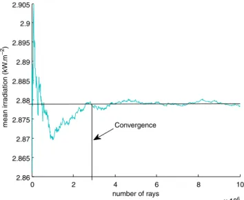
In more general case, when you simulate the infrared heating step of thermoforming process, you have not access to an exact solution. So, the error cannot be directly computed. An other advantage of stochastic method, is that you can also control the convergence of the computation. Figure11shows the convergence of the mean irradiation of the sheet. It can be seen that for three million rays, the convergence is obtained (2.88 kW.m−2). This type of figure allows a simple control of
the computation quality, even in the general 3D case. In 3D, the simplest indicator is the mean of the source term ∇.qr.
The ray tracing method is validated in the case of a sheet irradiated by one lamp. In the next subsection, we compare numerical results to experimental results in order to validate some physical assumptions before testing the ray tracing method in 3D complex cases of preform heating stage.
Comparison with experiment: sheet irradiation
In the previous sub-section, we have validated the di-rection definition of rays, in this new sub-section, we compare the results given by our ray tracing software, coupled with Comsol®(FEM) software, to experimen-tal results performed in [1,8] for the infrared heating stage of a rectangular sheet by IR lamps (Fig.13b). The lamp length is 280 mm and the nominal temperature
0 2 4 6 8 10 x 106 2.86 2.865 2.87 2.875 2.88 2.885 2.89 2.895 2.9 2.905 number of rays mean irr adiation (kW .m 2) Convergence
Fig. 11 Convergence of the ray tracing method
at 1,000 W is 2,400 K. This comparison is used to validate the assumption done on the ceramic reflector reflectance. Two cases of IR oven (Fig.12) are studied: the first one is the most simple oven composed by one single naked lamp (the single lamp oven) and the second one is an oven composed by three lamps with ceramic reflectors (the three lamps oven). Figure 13b shows lamps with and without ceramic reflector. In Fig. 12 is sketched the geometrical configuration of the ovens. In the single lamp case, only the central lamp is kept. We choose the example of the 3-mm thickness sheet because it is close to the thickness of the preform used for beverage bottles. The temperature measurement is done by IR camera.
The calculation of the temperature in the sheet is a 2-steps computation. In a first step, we compute the radiative source term (Eq.2), by using the ray tracing method, in all the sheet (3D). The radiative source term is then implemented into a commercial FEM software in order to solve the heat balance equation (Eq.5).
The boundary conditions used for the simulations are radiative and convective (Eq. 12). The sheet is a rectangular prism, so there are six faces: the face that is in front of the lamps is called the front face, the face that is at the opposite is called the rear face and the four other faces are called the border faces. The boundary condition for the border faces is thermal insulation. In order to simplify the calculation, the air temperature is assumed to be constant TAir= 22◦C and equal to the
initial temperature.
n(k∇T) = hi(TAir− T) + εPETσ (T4Air− T4)
i = front, rear (12)
Where εPET is the PET emissivity and it is equal to
0.93 [8] and σ = 5.67.10−8 W.m−2.K−4 is the
Stefan-Boltzmann coefficient. The heat transfert coefficient (natural convection) for the front face and the rear face
(a)
(b)
Fig. 13 a Prototype for stretch blow molding of the CROMeP
laboratory;b infrared lamps with and without ceramic reflector
are respectively hfront= 10 W.m−2.K−1 and hrear = 7
W.m−2.K−1[12]. The heating stage of the sheet is in two
steps. During a time theatthe preform is submitted to the
IR radiation of the oven, then oven is switched off and there is a cooling period during a time tcool. So, the total
time of the experiments is ttot= theat+ tcool.
For the single lamp oven, the heating time is theat=
65 s and the total time of the experiment is ttot= 110
s. In Fig.14the temperature versus time is plotted on two points of the sheet: the centers of the front and rear faces. There is a good agreement with the numerical simulation and experimental data. The mean square error, during the total time, is less than 5%.
For the temperature measurement on the front face, the IR camera has to take the place of the oven, in order to be in face-to-face with the front face. That is why experimental data on the front face begin after theat.
0 20 40 60 80 100 0 10 20 30 40 50 60 70 80 90 100 Time (s) Temper ature ( oC) 0 20 40 60 80 100 0 2 4 6 8 10 12 14 16 18 20 Error (%) Front (num) Rear (Num) Front (exp) Rear(exp) Front error Rear error
Fig. 14 Temperature variation in the center of the front and rear
faces versus time for the one lamp configuration
In order to validate the numerical model of the ceramic reflector, we now compare our ray tracing soft-ware to the experimental data obtained for the three lamps oven.
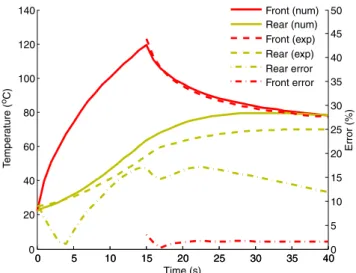
The Fig.15shows the temperature versus time in the center of the front and rear faces for the three lamps oven. In this case, the heating time is theat= 15 s and the
total time is ttot= 40 s. The agreement on the front face
is very good, the averaged error for theat≤ t ≤ ttotis less
than 2%. However, there is an overestimation of the temperature on the rear face. The error on the rear face is around 15%. Nevertheless, it is acceptable in light of the large number of parameters used in the simulation. A possible source of error can be the lamp modeling. Indeed, the emissivity of the tungsten is assumed to
0 5 10 15 20 25 30 35 40 0 20 40 60 80 100 120 140 Temper ature ( oC) 0 5 10 15 20 25 30 35 400 5 10 15 20 25 30 35 40 45 50 Time (s) Error (%) Front (num) Rear (num) Front (exp) Rear (exp) Rear error Front error
Fig. 15 Temperature versus time in the center of the front and
be constant. This assumption changes the way that the PET absorbs the energy emitted by IR lamps.
By comparing the two previous results, we can vali-date the modeling of the ceramic reflector proposed in [8]. In order to confirm the capabilities of the ray trac-ing method, we present, in the next section, simulations of the infrared heating stage of stretch blow molding process and we compare this results with experimental measurements.
Infrared heating stage of PET preform
Trials used in this paper have been performed by Monteix [8] on the stretch blow molding prototype of the CROMeP laboratory (Fig.13). Before the presen-tation of a complex heating case, we propose to study the case of a static preform. Figure16 illustrates the configuration of the oven used in the CROMeP pro-totype. The aluminum reflectors shown on the Fig.13 have been removed for the trials used in this study.
The oven is constituted of six halogen lamps (each had been set to a power of 1,000 W) with ceramic reflectors on the back. The use of a static preform al-lows us to study the propagation of rays through the two thicknesses of the preform. In fact, the preform having a hollow body, a ray may pass through two thicknesses of material before leaving the preform. The radiative source term ∇.qrobtained by the ray tracing method is
shown on Fig.17. The computational time of the source term is 90 min for the six lamps (6 × 2 million rays). This time can be decomposed into sub-time: the first one is the time of the geometrical calculation (60 min) and the second one is the time of power calculation (30 min). If
Fig. 16 Oven configuration for the infrared heating of PET
preform
Fig. 17 Source term computed in our software then used in
Comsol
only powers of the lamps are changed, the geometrical definition of rays can be kept and the computational time for the source term is reduced to 30 min. The source term will be used for the two next simulations.
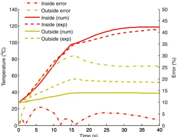
The Fig.18shows the temperature variation versus time for two points on the preform. The points are at mid-height of the preform. The first one is inside the preform in front of the lamps and the second one is outside the preform at the opposite of the lamps. So, we can evaluate the absorption in the two thicknesses of the preform.
Like in the heating stage of sheets, in the previous section, the heating stage of the preform is in two times: an heating time theatfollowing by a cooling time tcool. In
order to measure the temperature inside and outside
0 5 10 15 20 25 30 35 40 0 20 40 60 80 100 120 140 Temper ature ( oC) 0 5 10 15 20 25 30 35 400 5 10 15 20 25 30 35 40 45 50 Time (s) Error (%) Inside error Outside error Inside (num) Inside (exp) Outside (num) Outside (exp)
Fig. 18 Temperature versus time inside and outside of the PET
the preform, the experimental temperature acquisition is made in two steps. The first one is the acquisition of the inside temperature. During the heating time, the acquisition is made on a semi-preform: preform are be-forehand cut in two equal parts along the preform axis. On Fig.16, only the right part of the preform is kept. The second step of the temperature acquisition is made on an other preform, this is the outside temperature measurement.
As in the experimental protocol, the numerical sim-ulations are made on a semi preform and on an entire preform. The biggest difference between the two simu-lations are the boundary conditions on the inside face. In the first case, radiative and convective boundary conditions are applied. In the second case, thermal insulation is applied on the inside face. In both cases, the outside face is submitted to radiative and convective boundary conditions. The convections coefficients are the same as in the previous section. On the outside face, the convection coefficient is equal to 10 W.m−2 and
on the inside face, when is it applied, the convection coefficient is equal to 7 W.m−2. The radiative flux
boundary condition is the same on the inside (when it is applied) and on the outside faces and it is equal to εPETσ (T4Air− T4)with TAir= 27◦C.
Results of the simulations are shown on Fig.18. The computational time in Comsol® is 1 min for 12,000 degrees of freedom. A good agreement is obtained for the inside temperature: the error is around 5% during the heating period and the cooling period. In addi-tion, the error between the experimental temperature and the simulated temperature is around 25% on the outside face. This significant error can be explained by the results obtained for the sheet in the previous section. Indeed, for the sheet, the temperature on the rear face is overestimated, it means that the sheet had absorbed too much energy. If there was a second sheet after the first one, it will have less energy that expected and the temperature in the second sheet will be underestimated. So, if the two thicknesses of the preform are compared to two parallel sheets with the same thickness, the error between experiment and sim-ulation is not really amazing. As in the sheet example, the constant emissivity of tungsten seems to be the principal error source.
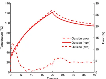
Now, we present the case of a rotating preform, this case is close to the industrial case. The biggest difference between the CROMeP prototype and indus-trial ovens is the translation of the preform across mul-tiple ovens. There is only one oven and no translation in the CROMeP prototype. The boundary conditions of this example are radiative and convective as in Eq.12) on the outside face, with hout= 10 W.m−2and thermal
0 5 10 15 20 25 30 35 40 0 20 40 60 80 100 120 140 Temper ature ( oC) 0 5 10 15 20 25 30 35 400 5 10 15 20 25 30 Time (s) Error (%) Outside error Outside (num) Outside (exp)
Fig. 19 Temperature versus time at mid-height of preform
(out-side face)
insulation on the inside face. The rotational speed is 1.2 round per second, the heating time is theat= 20 s and
the cooling time is tcool= 20 s.
The source term used for the rotative preform is the same as the one used for the static preform (Fig.17). An easy way to compute the rotation is not to consider a rotative preform in an oven, but it is to consider a rotative oven round a preform. So, only one calculation of source term is needed and the rotation of the source term shown on Fig.17is used for our simulations.
In Fig.19the temperature versus time is plotted on one point of the outside face at mid-height of the pre-form. The computational time in Comsol is 3 min. The agreement between the experiment and the simulation is better as in the previous case, the error is around 5%. The rotation of the source term works as an averaging. So, if there is an overestimation on one side and an underestimation on the other side, the error vanishes by rotation.
Conclusions and prospects
In this work, we have developed the ray tracing method in order to compute the radiative source term in IR heating problem. We first compared the ray tracing method with view factor in in case where exact solution is known for view factor and we proved the efficiency of the ray tracing method. In a second time, the ray tracing method is compared to basic experiments in order to validate some physical assumptions. Then, the simulation of a complex oven and the rotation of a preform is computed. This final comparison shows the capability of the ray tracing method to predict temperature distribution for stretch blow molding and
thermoforming processes of semi-transparent materi-als. We have shown that the good knowledge of the radiative properties of emitter (emittance) and receiver (absorption) is needed to provide good estimation of the temperature field.
The next evolution of the software is the introduc-tion of our own spectral data for the emissivity of tungsten. New experiments will be performed in order to measure the emissivity for all the emission range. Some work (experimental or theoretical) exist, but the emissivity is just given for a part of the emission spec-trum of tungsten. Desvignes [3] gives the emissivity for wavelengths to 2.6 µm and [14] gives the emissivity for wavelengths from 2.6 µm.
The next steps of this study is the coupling of the thermal calculation with mechanical calculation in or-der to provide a tool which is able to predict the final bottle properties. This tool would be able to help en-gineers to find the good process conditions in order to make good bottles (thickness, mechanical properties).
Acknowledgement This work could not be possible without our
industrial partner: O. Demangeon from Toshiba Lighting.
References
1. Champin C (2007) Modélisation 3d du chauffage par rayon-nement infrarouge et de l’étirage soufflage de corps creux en p.e.t. Ph.D. thesis, École des Mines de Paris
2. Cosson B, Chevalier L, Yvonnet J (2009) Optimization of the thickness of PET bottles during stretch blow molding by using a mesh-free (numerical) method. Int Polym Process 03:223–233
3. Desvignes F (1997) Rayonements optiques. Masson, France 4. Erchiqui F, Hamani I, Charette A (2009) Modélisation par
éléments finis du chauffage infrarouge des membranes ther-moplastiques semi-transparentes. Int J Therm Sci 48(1): 73–84
5. Leuenberger H, Person RA (1956) Compilation of radiation shape factors for cylindrical assemblies. Presented at ASME Annual Meeting, New York, NY, Nov. 25–30, 1956
6. Mayhan K, James J, Bosch W (1965) Poly(ethylene tereph-talate). I. Study of crystallization kinetics. J Appl Polym Sci 9:3617–3624
7. Modest M (1993) Radiative heat transfer balbla. Elsevier Science
8. Monteix S (2001) Modélisation du chauffage convecto-radiatif de préformes en pet pour la réalisation de corps creux. Ph.D. thesis, École des Mines de Paris
9. Monteix S, Maoult YL, Schmidt F, Arcens JP (2004) Quan-titative infrared thermography applied to blow moulding process: measurement of a heat transfer coefficient. QIRT J 1(2):133
10. Monteix S, Schmidt F, Maoult YL, Yedder RB, Diraddo RW, Laroche D (2001) Experimental study and numerical simulation of preform or sheet exposed to infrared radiative heating. J Mater Process Technol 119(1–3):90–97
11. Pharr M, Humphreys G (2004) Physically based rendering: From theory to implementation. Elsevier Science, USA 12. Sacadura J (1973) Initiation aux transferts thermiques.
Lavoisier, France
13. Schmidt F, Agassant J, Bellet M (1998) Experimental study and numerical simulation of the injection stretch/blow mold-ing process. Polym Eng Sci 38(9):1399–1412
14. Siegel R, Howel J (1992) Thermal radiation heat transfer. Hemisphere Publishing Corporation, USA
![Fig. 2 Spectral absorption coefficient κ λ [9]](https://thumb-eu.123doks.com/thumbv2/123doknet/12569661.345737/3.892.459.811.781.1087/fig-spectral-absorption-coefficient-κ-λ.webp)
![Fig. 3 Spectral reflection r λ of PET [8]](https://thumb-eu.123doks.com/thumbv2/123doknet/12569661.345737/4.892.461.815.122.361/fig-spectral-reflection-r-λ-pet.webp)