Knowledge-aided STAP in heterogeneous clutter using a hierarchical bayesian algorithm

Any correspondence concerning this service should be sent to the repository administrator: [email protected]

O

pen

A

rchive

T

oulouse

A

rchive

O

uverte (

OATAO

)

OATAO is an open access repository that collects the work of Toulouse researchers

and makes it freely available over the web where possible.

This is an author -deposited version published in:

http://oatao.univ-toulouse.fr/

Eprints ID: 4909

To link to this article: DOI:

10.1109/TAES.2011.5937270

URL:

http://dx.doi.org/10.1109/TAES.2011.5937270

To cite this version: BIDON Stéphanie, BESSON Olivier, TOURNERET Jean-Yves

Knowledge-aided STAP in heterogeneous clutter using a hierarchical bayesian algorithm.

IEEE Transactions on Aerospace and Electronic Systems, 2011, vol. 47, n° 3, pp. 1863

-1879. ISSN 0018-9251

Knowledge-Aided STAP in

Heterogeneous Clutter using

a Hierarchical Bayesian

Algorithm

ST ´EPHANIE BIDON, Member, IEEE OLIViER BESSON, Senior Member, IEEE

University of Toulouse, ISAE

JEAN-YVES TOURNERET, Senior Member, IEEE

University of Toulouse, IRIT/ENSEEIHT France

The problem of estimating the covariance matrix of a primary vector from heterogeneous samples and some prior knowledge is addressed, under the framework of knowledge-aided space-time adaptive processing (KA-STAP). More precisely, a Gaussian scenario is considered where the covariance matrix of the secondary data may differ from the one of interest. Additionally, some knowledge on the primary data is supposed to be available and summarized in a prior matrix. Two KA-estimation schemes are presented in a Bayesian framework whereby the minimum mean square error (MMSE) estimates are derived. The first scheme is an extension of a previous work and takes into account the nonhomogeneity via an original relation. In search of simplicity and to reduce the computational load, a second estimation scheme, less complex, is proposed and omits the fact that the environment may be heterogeneous. Along the estimation process, not only the covariance matrix is estimated but also some parameters representing the degree of a priori and/or the degree of heterogeneity. Performance of the two approaches are then compared using STAP synthetic data. STAP filter shapes are analyzed and also compared with a colored loading technique.

I. INTRODUCTION

Detecting targets in highly heterogenous

environments is a challenging task for future airborne radars. Signal processing has to enable the extraction of targets embedded in noise consisting mostly of thermal noise, possibly jammers, and ground clutter whose characteristics may vary rapidly over azimuth and range. Space-time adaptive processing (STAP) is recognized today as the best candidate to perform this task [1—3]. STAP performance depends mostly on the knowledge of the noise covariance matrix. As the noise cannot entirely be known a priori, its covariance matrix is usually estimated from secondary range cells. In a homogeneous environment, where the range gates share the same covariance matrix, the sample covariance matrix (SCM) maximizes the signal-to-noise-plus-interference ratio (SINR) [4] and is also the maximum likelihood estimator [5]. Unfortunately, in real-world scenarios, the homogeneity assumption is often not satisfied. Thus the SCM may be a poor estimate of the true noise covariance matrix.

Heterogeneity can be caused by many phenomena [6, 7] including nonhomogeneous ground reflectivity (e.g., amplitude and/or spectral variation, clutter edges, discretes), secondary targets in the training interval or in the cell under test, and range-dependence of the clutter frequencies in the angle-Doppler domain (often referred to as nonstationary clutter). A variety of models have been proposed to measure the impact of several types of heterogeneity. Most of them rely on the general clutter model (GCM) covariance matrix developed by the radar community [1]. Thus, amplitude and spectral variations but also target-like signals in the secondary data can severely compromise STAP performance [8]. Highly nonstationary clutter can lead as well to very poor detection performance around clutter angle-Doppler loci [2].

Many techniques have been considered to counteract the deleterious effect of heterogeneity. Low sample support algorithms intend to reduce the presence of heterogeneous samples in the training interval. Among them one can mention reduced rank or reduced dimension algorithms [1, 2, 9], diagonal loading [10], and estimation schemes based on structured interferences [11, 12]. On the other hand, a careful selection of the secondary data allows one to discard heterogeneous samples according to a certain criterion based, e.g., on power considerations [13] or on more complex metrics such as nonhomogeneity detectors (NHD) [14]. Another way to deal with heterogeneity is to incorporate it directly via a model into the detection scheme. Some detectors for instance allow one to take into account local power fluctuations [15, 16]. However, one of the most promising ways to enhance the detection performance in heterogenous environments may be the use of a priori knowledge.

Such algorithms are referred to as knowledge-aided STAP (KA-STAP) and are often merged with the former cited strategies.

This last decade KA-processing has received a growing interest and seems to be a key concept for the next generation of adaptive radar systems [17, 18]. In this sense, the Defense Advanced Research Projects Agency (DARPA) has initiated the KA sensor signal processing and expert reasoning (KASSPER) workshop [19]. KA-STAP aims at using prior knowledge provided by external databases (e.g., digital ground model, Global Positioning System (GPS), previous scanning data) to assist and improve detection. The a priori information can be used in two ways [20, 21]: either indirectly, e.g., to select representative training data [22, 23], or directly to form the filter. Regarding this last concern, it is generally assumed that the prior information can be summarized into a known matrix. This matrix is often built upon the GCM, where parameter values have been set up at the system design stage or by measurements. One delicate issue is then to adequately use this a priori matrix to form the STAP filter.

Among the algorithms that allow one to incorporate the a priori matrix into the detection scheme, one can mention the fast maximum likelihood with assumed clutter covariance [24], the KA

parametric estimation [25] and colored loading (CL). CL is a commonly used technique whereby the covariance matrix estimate is formed as a weighted sum of the SCM and the a priori covariance matrix [26—33]. CL has an appealing form because the STAP filter can be implemented in two steps: a prewhitening step based on the prior matrix, followed by adaptive filtering [34]. Interestingly, the technique happens to be the solution to different problem formulations. In [27], [28], [34], CL is presented as the solution of the usual linearly constrained minimum variance space-time beamformer with an additional quadratic constraint. In [35]—[37], a Bayesian approach is undertaken instead and leads also to the CL technique. Though CL seems to be an efficient method to

incorporate a priori information, the choice of the weighting factors remains a delicate issue and is discussed in [21], [31], [32]. An adaptive approach seems obviously more adequate. In [21], the weight of the prior matrix is derived so as to maximally whiten the observed interference data. In [31], a maximum-likelihood approach is invoked under the restrictive assumption that the weighting factors are range independent. In [32], this restrictive assumption is alleviated, and the weights are derived so as to minimize the mean-squared error (MSE) of the CL estimator.

Recently, so as to integrate the prior matrix in the estimation scheme, we have focussed our attention on a new Bayesian data model [33, 38]. The Bayesian approach turns out to be appropriate both to take

into account the nonhomogenous assumption (in a certain way) and to incorporate the prior matrix. The proposed model is tuned by two scalars called hyperparameters that were shown to represent the degree of heterogeneity of the environment and the degree of a priori knowledge. In [38], the minimum mean-squared estimator (MMSE) of the noise covariance matrix is derived, assuming these two scalars are exactly known. Obviously, for practical applications, these quantities are unknown and have to be chosen properly. To do so, we propose here to extend the work of [38] by introducing a hierarchical level to the data model. More precisely, we consider both the degree of heterogeneity and the degree of a priori knowledge as random variables with known priors and estimate them jointly with the covariance matrix. This new estimation strategy is therefore a robustified version of the algorithm presented in [38]. After describing the robustified algorithm thoroughly, we study its performance for a STAP scenario. Particularly, we intend to observe the STAP filter shape and the values of the estimated hyperparameters to highlight how the prior information is incorporated and how the heterogeneity is dealt with. Note that we do not focus our attention on the generation of the prior matrix (though a major topic). Additionally, we propose another robustified algorithm in the case where the heterogeneity would not be taken into account and show that this omission can lead to severe loss. This could happen for instance if, after an NHD, some heterogeneous samples still remained in the training interval.

The remainder of the paper is organized as follows. Section II describes the Bayesian data model and the robustified estimation procedure originally introduced in [39]. Section III presents a similar algorithm, but this algorithm alleviates the heterogeneous assumption so as to obtain less complex estimators. Section IV provides

numerical results obtained from synthetic STAP data. Conclusions and perspectives are finally drawn in Section V.

II. KNOWLEDGE-AIDED ESTIMATION IN A HETEROGENEOUS ENVIRONMENT This section describes the data model for a KA-heterogenous environment with its MMSE estimation procedure initially introduced in [39]. The model, defined under a Baysesian framework, entails two original relations, one describing the heterogeneity of the environment and the other describing how the prior information is related to the primary data. These two relations are partly chosen to ensure mathematical tractability. Thus, so as to robustify the model, we turn to a common strategy encountered in the Bayesian philosophy, the hierarchical Bayes modeling [40]. More precisely, an additional hierarchical level is added to the data

model whereby the hyperparameters–representing the degrees of heterogeneity and a priori of the model–are considered as random variables with noninformative priors.

A. Data Model

We intend to estimate the covariance matrix

M_p of a ³-length complex data vector z with both K secondary data Z = [z_1¢¢¢zK] and some a priori information collected into a prior matrix ¯M_p. As a first attempt to model heterogeneity, the z_ks are supposed to be independent and Gaussian distributed with the same covariance matrix M_s, which may differ from M_p. This distribution is denoted by

Z_{j Ms» ˜N³,K}(0, M_s): (1) The probability density function (pdf) of Z_{j Ms} is thus given by

f(Z_{j Ms}) = ¼¡³K_jMsj¡Ketr_{f¡M ¡ s}¡1S_g (2) where S = ZZH,_{j:j and etrf:g stand for the}

determinant and the exponential of the trace of a matrix, respectively. To complete the data model, a Bayesian framework is then advocated so that both the primary and secondary covariance matrices are considered as random variables with known priors. Choosing these two priors is rather delicate. As presented hereafter, we have chosen Wishart and inverse Wishart distributions. These priors have already been invoked under statistical considerations in similar contexts [41, 42]. In a first step, the two priors are designed so that the primary matrix M_p departs possibly from the secondary covariance

M_s and/or from the prior matrix ¯M_p. The pdfs are also chosen among conjugate priors to make the model suitable for further derivations. In a second step, a hierarchical level is added to robustify these conjugate prior distributions, i.e., making the model less sensitive to the choice of these two priors.

1) Heterogeneity Model: Unlike the physical-based model [1], the heterogeneity is

described here by the pdf of the secondary covariance matrix M_s which has to be thoroughly designed. A complex inverse Wishart distribution–with º degrees of freedom and associated covariance matrix (º_{¡ ³)Mp}–is chosen as an adequate candidate and is denoted by M_{sj Mp}, º_{» ˜W³}¡1((º_{¡ ³)Mp}, º) (3) with pdf f(M_{sj Mp}, º) = j(º ¡ ³)Mpj º ˜ ¡_³(º)_jMsj(º+³)etrf¡(º ¡ ³)MsMpg (4) where ˜ ¡_³(º) = ¼³(³¡1)=2 ³ Y k=1 ¡ (º_{¡ ³ + k)} (5)

and where ¡ (:) is the gamma function. To be correctly defined, º has to be greater than or equal to ³, and the parameter matrix has to be Hermitian positive definite (i.e., º > ³).

The distribution (3) implies that on average the environment is homogenous, i.e.,_{EfMsj Mp}, º_{g = Mp}, but ensures that M_s always differs from M_p. Looking now at the second-order moment, it is clear that the hyperparameter º monitors the distance between M_p and M_s via the relation

Ef(Ms¡ Mp)2_{j Mp}, º_{g =}M 2

p+ (º¡ ³)TrfMpgMp (º_{¡ ³ + 1)(º ¡ ³ ¡ 1)} :

(6) The larger º is, the more homogeneous the

environment. Thus, in the following, the hyperparameter º is referred to as the degree of heterogeneity of the environment. Note also that the former expression (6) is defined only if º > ³ + 1.

Of course we do not pretend here that the model (3) can embrace every kind of heterogeneity, especially because some limitations can be expected due to the fact that_{EfMsj Mp}, º_{g = Mp} [38]. However, as shown in the numerical Section IV, model (3) is actually able to take into account, in an interesting way, the fact that M_{s6= Mp}.

2) KA Model: The KA part of the model is described in a similar way to the heterogeneous model. Note that some authors [41] have previously proposed a Bayesian KA model involving a primary covariance matrix M_p and a random prior matrix

¯

M_p. Indeed, given that ¯M_p could be based on prior Gaussian observations, they have assumed that ¯M_pj M_p has a Wishart distribution with mean M_p. Here, we have assumed that the primary covariance matrix

M_p is a random variable distributed around an ideal and known matrix ¯M_p that is built upon relevant models and databases. Randomness allows the primary matrix M_pto absorb some real effects or model inaccuracies not foreseen in the prior matrix ¯M_p(e.g., calibration errors, near-field effects, inaccuracies of GPS and/or cultural databases, etc.). More precisely, the covariance matrix M_p is supposed to be drawn from a complex Wishart distribution denoted by

M_{pj ¯}M_p, ¹_{» ˜W³}(¹¡1M¯_p, ¹) (7) with pdf f(M_{pj ¯}M_p, ¹) = jMpj ¹¡³ ˜ ¡_³(¹)_j¹¡1_M¯_pj¹etrf¡¹Mp ¯ M¡1_{p g:} (8) Note here that the prior matrix ¯M_p is supposed to be Hermitian positive definite and stands for the whole noise (not only the ground clutter). Also, the hyperparameter ¹ has to be greater than or equal to ³.

The distribution (7) implies that on average the primary covariance matrix is equal to the a priori

matrix, i.e.,_{EfMpj ¯}M_p, ¹_{g = ¯}M_p, but ensures that

M_p differs from ¯M_p. Besides, observing the second order moment, one notices that the hyperparameter ¹ monitors the distance between M_p and ¯M_p via the relation

Ef(Mp¡ ¯M_p)2_{j ¯}M_p, ¹_{g =} Trf ¯Mpg ¹

¯

M_p: (9)

The larger ¹ is, the more accurate the prior

information. Hence the hyperparameter ¹ is referred to as the degree of a priori knowledge.

3) Hyperparameters: Thus far, we have established a KA-heterogenous model whereby two priors, (4) and (8), have been chosen among a family of conjugate priors to ensure mathematical tractability. In [38] and [33], we proposed an estimation procedure assuming that both the hyperparameters º and ¹ introduced by (4) and (8) were known. For practical applications, these two quantities are unknown and have to be chosen carefully, as estimation performance depends on their values. Therefore, we develop here a robustified version of the algorithm of [38], assuming that º and ¹ are random variables with noninformative priors. More precisely, we propose to consider them independent with uniform discrete pdfs, i.e.,

º_{j ºm}, º_{M» Ufºm,:::,ºMg} (10a) ¹_{j ¹m}, ¹_{M» Uf¹m,:::,¹Mg} (10b) where º_m, º_M, ¹_m, and ¹_M are integers setting the bounds of the estimation.

We discuss here the values of the bounds º_m, º_M, ¹_m, and ¹_M. Assuming that no information is available either on the degree of heterogeneity or on the degree of a priori knowledge, one has to take care that (10a) and (10b) are noninformative priors. In other words, intervals_fºm, : : : , º_{Mg and} f¹m, : : : , ¹_{Mg must have a good dynamic range to} represent every possible degree of heterogeneity and a priori, respectively. As explained before, the values of the integers º and ¹ have to verify º > ³ and ¹_{¸ ³, respectively, and so do the lower-bounds,} i.e., º_{m¸ ³ + 1 and ¹m¸ ³. Discussing the values of} º_M and ¹_M is a little bit more delicate. Indeed, the values of º and ¹ are not a priori upper bounded. Yet, looking at (6) and (9), the distance between the two matrices at stake is approximately (or exactly) inversely proportional to the hyperparameter. Thus, beyond a certain value of º (respectively ¹), the heterogeneity of the environment (respectively the accuracy of the prior matrix) does not change much. An opposite behavior is observed for small º and ¹. Hence it is crucial to adjust the minimal bounds º_m and ¹_m as low as possible, i.e., º_m= ³ + 1 and ¹_m= ³. Furthermore, the heterogeneity of the environment and the accuracy of the prior knowledge are not misrepresented if one compells

º and ¹ to lie in appropriate upper-bounded intervals. We see later that the numerical choice of º_M and ¹_M also strongly drives the required computational resources.

For the sake of convenience, we omit in the rest of the paper constant and known quantities in the conditional terms.

B. MMSE Estimation

1) Monte Carlo Method: We present here the joint MMSE estimation of the matrix M_p and the hyperparameters º and ¹ according to the model previously exposed. The notation μ is used to designate indifferently one of these variables. By definition, the MMSE estimate of μ is the average of the posterior distribution1

ˆ

μmmse=_{Efμ j Zg =} Z

μf(μ_{j Z)dμ:} (11) As explained in [39], the derivation of the integral (11) is feasible for neither M_p, nor for º or ¹. Moreover, resorting to deterministic methods (such as numerical integration) to approximate (11) has to be prohibited when the problem dimension is greater than 4 [43], which is always the case in STAP applications. As a consequence, we propose the use of a Markov chain Monte Carlo (MCMC) method to generate samples distributed according to an appropriate target distribution and to use the samples to approximate Efμ j Zg. More precisely, a hybrid Gibbs sampler [44] can be used to generate samples (M(i)

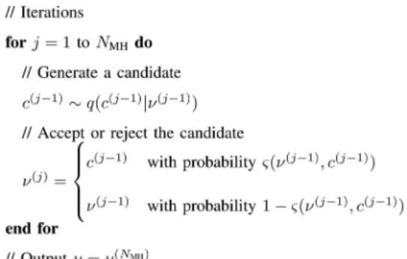
p , M(i)s , º(i), ¹(i)) distributed according to the joint posterior distribution f(M_p, M_s, º, ¹_{j Z). As described in Fig. 1, each} sample μ(i)_{is generated according to its conditional} distribution. After a burn-in period–say, equal to N_bi samples–the iterative process generates samples μ(i) distributed according to their posterior distribution f(μ_{j Z) [44]. Thus, the MMSE estimates of μ can be} approximated by the empirical mean

ˆ μmmse ¢= 1 N_r Nr X i=1 μ(i+Nbi) ₍₁₂₎ where N_r is a number of samples ensuring that the estimate will be correctly approximated. The values of the burn-in period N_bi and the number of samples of interest N_r are discussed later in Section IV. Note that the convergence of the procedure is obtained with whatever initial value μ(0) _{is supplied [44]. For} instance, in Fig. 1, º(0) and ¹(0) are chosen randomly according to (10a) and (10b), and M(0)_p is chosen as the SCM given by ˆ Mscm p = 1 KS:

1_{Let us remind readers here that, so as to lighten the expressions,}

constant and known parameters (e.g., ¯M_p, º_m, º_M, ¹_m, and ¹_M) are not mentioned in the conditional terms.

Fig. 1. Hybrid Gibbs sampler.

Note also that the MMSE of the secondary covariance matrix M_s can be obtained as a byproduct of the proposed sampling strategy.

To derive the conditional distribution of each chain parameter, we first express the joint posterior distribution of M_p, M_s, º, ¹_{j Z. Using the Bayes} theorem with (2), (4), (8), and (10), one obtains

f(M_p, M_s, ¹, º_{j Z)} / jMsj¡(º+³+K)jMpjº+¹¡³j ¯M_pj¡¹ £ etrf¡M ¡ s¡1_{[S + (º¡ ³)Mp]¡ ¹ ¯M}¡1 p Mpg £(º¡ ³) ³º ˜ ¡_³(º) ¹³¹ ˜ ¡_³(¹) I fºm,ºMg(º)If¹m,¹Mg(¹) (13) where I_fa,bgis the indicator function defined on the set of integers_{fa,:::,bg and / means proportional to.}

2) Gibbs Moves: We use the expression (13) to obtain the conditional distributions of M_{pj Ms}, º, ¹, Z and M_{sj Mp}, º, ¹, Z. Considering, M_s, º, and ¹ as given quantities in (13), it follows that

f(M_{pj Ms}, º, ¹, Z)

/ jMpjº+¹¡³etr_{f¡[¹ ¯}M¡1_p + (º_{¡ ³)M ¡ s}¡1]M_pg: (14) Similarly, one can show that

f(M_{sj Mp}, º, ¹, Z)

/ jMsj¡(º+K+³)etr_{f¡M ¡ s}¡1[S + (º_{¡ ³)Mp}]_g: (15) Therefore, the conditional distributions of M_{pj Ms}, º, ¹, Z and M_{sj Mp}, º, ¹, Z are recognized as complex

Wishart and inverse complex Wishart distributions, respectively,

Mpj Ms, º, ¹, Z» ˜W³([¹ ¯M¡1p + (º¡ ³)M ¡ s¡1]¡1, º + ¹)

(16a)

M_{sj Mp}, º, ¹, Z_{» ˜W³}¡1(S + (º_{¡ ³)Mp}, º + K): (16b) Complex Wishart and inverse complex Wishart

distributions can be easily sampled to generate the matrices M(i)

p and M(i)s . These two steps are referred to as Gibbs moves.

3) Metropolis-Hastings Moves: Let us consider now the generation of samples º(i) _{and ¹}(i)_{. Using} (13), the conditional distributions of º_{j Mp}, M_s, ¹, Z and ¹_{j Mp}, M_s, º, Z can be expressed as

f(º_{j Mp}, M_s, ¹, Z) /(º¡ ³) ³º ˜ ¡_³(º) jMpM¡ s ¡1_jº £ etrf¡(º ¡ ³)MpM_{¡ s}¡1_gIfº m,ºMg(º) (17a) f(¹_{j Mp}, M_s, º, Z) / ¹ ³¹ ˜ ¡_³(¹)jMp ¯ M¡1_{p j}¹etr_f¡¹MpM¯¡1_{p gIf¹m,¹Mg}(¹): (17b) Unfortunately the pdfs (17) do not belong to any familiar class of distributions. Therefore, we resort to a Metropolis-Hastings (MH) move [44]. The MH algorithm is an iterative procedure that generates samples asymptotically distributed according to a given target distribution. Its principle is explained hereafter.

Let us focus, for instance, on the target distribution g (third step in Fig. 1), given by

g(º) = f(º_{j M}(i)_p, M(i)_s , ¹(i¡1), Z): The MH algorithm associated with this target distribution is described in Fig. 2 for N_MH iterations. At the jth iteration, a candidate c(j¡1)is drawn from a proposal distribution q(:_{j º). The candidate c}(j¡1)is then accepted as the next sample º(j) _{according to the} acceptance probability &(º(j¡1), c(j¡1)) = min ½ 1,g(c (j¡1)₎ g(º(j¡1)₎ q(º(j¡1)_{j c}(j¡1)) q(c(j¡1)_{j º}(j¡1)₎ ¾ : (18) The proposal distribution q(:_{j º) has to be chosen} properly. First, from an implementation point of view, q(:_{j º) has to be easy to sample. Additionally,} any proposal distribution q(:_{j º) can be chosen as} long as its support contains the support of the target distribution [45]. Then, two routes are usually taken. The first approach is referred to as a random-walk MH algorithm. Candidates are of the form c(j)_{= º}(j)

Fig. 2. MH algorithm (implementation of step 3).

+" where " is a random variable with an appropriate distribution [44]. This technique is well suited for narrow target distributions. As depicted in Fig. 3, the target distribution (17) is quite narrow for small values of º but becomes much wider for larger values of º. We thus turn to the second approach based upon an independent proposal mechanism whereby the candidate does not depend on the instantaneous chain sample [44, p. 276]. More precisely, to fulfill the former requirements and in search of simplicity, we choose a uniform proposal distribution as in (10a), i.e.,

q(c(j¡1)_{j º}(j¡1)) = q(c(j¡1))_{/ Ifºm,ºMg}(c(j¡1)): (19) This way, the proposal distribution is able to explore the support of the target distribution equally likely. This is desirable, as it is assumed that no information is available about the true value of º. The MH acceptance probability (18) boils down to

&(º(j¡1), c(j¡1)) = min ½ 1,g(c (j¡1)₎ g(º(j¡1)₎ ¾ (20) meaning that the candidate is always accepted if it contributes to increasing the target distribution. Note that the convergence time of the MH algorithm will increase according to the length of the interval fºm, : : : , º_{Mg, as the algorithm must explore the whole} support of the target distribution. Recalling that we have earlier set º_m= ³ + 1, this means that, from a computational point of view, º_M must be kept as low as possible. Similar reasonings can be made for the fourth step of the sampler leading to q(¹0_{j ¹) /} I

f¹m,¹Mg(¹ 0_).

Finally, note an interesting property of the hybrid Gibbs sampler depicted in Fig. 1. As explained before, the MH algorithm is an asymptotic procedure. Hence, several accept/reject procedures usually have to be performed before the samples become actually distributed according to the target distribution, i.e., N_{MHÀ 1. Conversely, the convergence of the hybrid} Gibbs sampler is achieved even when steps 3 (and

Fig. 3. Theoretical posterior conditional distribution of ºj Mp, Ms, ¹, Z. KA-heterogeneous model. K = 24, ¹min= 9,

¹_max= 40.

4) are reduced to a single accept/reject step [43], i.e., N_MH=1.

III. KNOWLEDGE-AIDED ESTIMATION IN A HOMOGENOUS ENVIRONMENT

In the previous section, a KA-estimation procedure for use in a heterogenous environment has been described. One could argue against its complexity or the fact that the heterogeneity part of the model is not, strictly speaking, physical based. We intend to investigate in this section the relevance of the heterogeneity relation (3). Is it worth introducing it in the estimation scheme? To answer that question, we develop a similar estimation procedure based on a model that alleviates the heterogenous assumption. More precisely, we assume that M_p= M_s, and we still consider that some prior information is available and summarized into the matrix ¯M_p. After adjusting the model of Section II to a homogeneous case, we derive the MMSE estimators of both M_p and ¹ that are obtained enjoyably in closed form. Note that the KA-homogeneous model presented in this section turns out to be a robustified version of the one described in [36], [37], where the parameter ¹ was assumed to be known. Comparison of the KA-heterogeneous and KA-homogeneous models is performed in Section IV.

A. Data Model

Under the assumption of a homogeneous environment, the secondary data Z share the same covariance matrix M_p as the primary data z, i.e.,

Z_{j Mp» ˜N³,K}(0, M_p): (21) To ensure mathematical tractability, the matrix M_p is supposed to be drawn from an inverse Wishart

distribution (a similar reasoning is made in [36], [37]). Indeed, this way, the distribution of M_{pj ¯}M_p, ¹ is a conjugate prior for the likelihood f(Z_{j Mp}). To establish a certain fairness for further comparison with the KA-heterogenous model introduced earlier, the parameters of this distribution are adjusted to ensure EfMpj ¯M_p, ¹_{g = ¯}M_p, i.e.,

M_{pj ¯}M_p, ¹_{» ˜W³}¡1((¹_{¡ ³) ¯}M_p, ¹): (22) The pdf of M_{pj ¯}M_p, ¹ is thus given by

f(M_{pj ¯}M_p, ¹) = j(¹ ¡ ³) ¯Mpj ¹ ˜ ¡_³(¹)_jMpj¹+³etrf¡(¹ ¡ ³)M ¡1 p M¯pg: (23) Note also that the hyperparameter ¹ can still be interpreted as the degree of a priori knowledge because we have for ¹ > ³ + 1,

Ef(Mp¡ ¯M_p)2_{j ¯}M_p, ¹_{g =} ¯ M2 p+ (¹¡ ³)Trf ¯Mpg ¯Mp (¹_{¡ ³ + 1)(¹ ¡ ³ ¡ 1))} : (24) The larger ¹ is, the more accurate the prior

information contained in the matrix ¯M_p.

To complete and robustify the KA-homogenous model, a hierarchical level is introduced via a noninformative prior on ¹. More precisely, we keep the former distribution (10b), whereby the hyperparameter is modeled as a uniform discrete random variable on an appropriate interval f¹m, : : : , ¹_{Mg, i.e.,}

¹_{j ¹m}, ¹_{M» Uf¹m,:::,¹Mg}:

Let us remind readers here that, by doing so, the prior of M_p, i.e., f(M_p) =R_¹f(M_{pj ¹)f(¹)d¹, is less} restrictive than a prior f(M_{pj ¹0}) where ¹ would have been set to an arbitrary constant ¹₀. Note that the domain of the definition of ¹ is now slightly different, i.e., ¹ > ³, and therefore ¹_m> ³.

B. MMSE Estimation

According to the KA-homogeneous data model (21), (22), and (10b), we derive now the MMSE estimators of the degree of a priori knowledge ¹ and the matrix M_p. Using the Bayes theorem, the joint posterior distribution of ¹, M_{pj Z can be expressed as} follows: f(¹, M_{pj Z) =} 1 f(Z) 1 ¼³K 1 ¹_{M¡ ¹m}+ 1 j(¹ ¡ ³) ¯M_pj¹ ˜ ¡_³(¹)_jMpjK+¹+³ £ etrf¡M¡1p [S + (¹¡ ³) ¯Mp]gIf¹m,¹Mg(¹): (25) We start by deriving the MMSE estimator of ¹

because the posterior distribution f(¹_{j Z) is useful} in expressing the MMSE estimator of M_p.

1) MMSE Estimator of ¹: Using (25), the posterior distribution of ¹_{j Z can be expressed as} follows: f(¹_{j Z) =} Z f(¹, M_{pj Z)dMp} /j(¹ ¡ ³) ¯Mpj ¹ ˜ ¡_³(¹) I f¹m,¹Mg(¹) Z ₁ jMpjK+¹+³ £ etrf¡M¡1p [S + (¹¡ ³) ¯Mp]gdMp (26) / j(¹ ¡ ³) ¯Mpj ¹ jS + (¹ ¡ ³) ¯M_pjK+¹ ˜ ¡_³(K + ¹) ˜ ¡_³(¹) I f¹m,¹Mg(¹) (27) where we have recognized in (26) the integral of an inverse Wishart distribution with parameter matrix

S + (¹¡ ³) ¯M_p and K + ¹ degrees of freedom. Finally, the posterior pdf of ¹_{j Z is given by}

f(¹_{j Z) = ¯c} j(¹ ¡ ³) ¯Mpj ¹ jS + (¹ ¡ ³) ¯M_pjK+¹ ˜ ¡_³(K + ¹) ˜ ¡_³(¹) I f¹m,¹Mg(¹) (28) where ¯c is a normalization constant such as

¯c¡1₌ ¹M X ¹=¹m j(¹ ¡ ³) ¯M_pj¹ jS + (¹ ¡ ³) ¯M_pjK+¹ ˜ ¡_³(K + ¹) ˜ ¡_³(¹) : (29) The MMSE of ¹ is then obtained in closed form as the mean of the posterior distribution (28)

ˆ ¹mmse= P¹M ¹=¹m¹h(¹) P¹M ¹=¹mh(¹) (30) where h(¹) = j(¹ ¡ ³) ¯Mpj ¹ jS + (¹ ¡ ³) ¯M_pjK+¹ ˜ ¡_³(K + ¹) ˜ ¡_³(¹) : (31) Observing (30), we can note that if ¹_M= ¹_m then ¹ is a deterministic quantity and, as expected, ˆ¹mmse₌ ¹_M= ¹_m.

REMARK1 (Implementation issue) To avoid

numerical problems, we recommend computing ˆ¹mmse as follows: ˆ ¹mmse= P¹M ¹=¹m¹˜h(¹) P¹M ¹=¹m˜h(¹) (32) where ˜h(¹) = exp_{flog(h(¹)) ¡ log(h( ˜¹))g and ˜¹ =} arg max_¹log h(¹).

2) MMSE Estimator of M_p: Using (25), the conditional posterior distribution of M_{pj Z,¹ can be} expressed as f(M_{pj Z,¹) /}etrf¡M ¡1 p [S + (¹¡ ³) ¯Mp]g jMpjK+¹+³ If¹m,¹Mg(¹): (33)

We thus recognize that M_{pj Z,¹ is distributed} according to the following inverse Wishart distribution:

M_{pj Z,¹ » ˜W³}¡1(S + (¹_{¡ ³) ¯}M_p, K + ¹): (34) Using the hierarchical structure of the data model, the posterior pdf of M_{pj Z can be written as the finite} sum f(M_{pj Z) =} ¹M X ¹=¹m f(M_{pj Z,¹)f(¹ j Z):} (35) Averaging the pdf (35), we obtain the MMSE

estimator of M_p: ˆ Mmmse p = Z M_p ¹M X ¹=¹m f(M_{pj Z,¹)f(¹ j Z)dMp} = ¹M X ¹=¹m EfMpj Z,¹gf(¹ j Z): (36) EfMpj Z,¹g is the mean of the inverse Wishart distribution (34), i.e.,_{EfMpj Z,¹g = [S + (¹ ¡ ³) ¯}M_p]= (K + ¹_{¡ ³). The MMSE estimator of Mp}can finally be obtained in closed form by

ˆ Mmmse_p = w ˆMscm_p + ¯w ¯M_p (37) where w = ¹M X ¹=¹m K K + ¹_{¡ ³}f(¹j Z) (38a) ¯ w = ¹M X ¹=¹m ¹_{¡ ³} K + ¹_{¡ ³}f(¹j Z): (38b) To give some insight to the former expression (37), several remarks can be made.

1) The MMSE estimate of M_p is equivalent to an adaptive CL technique where the weights of each matrix depend on the data through the posterior distribution f(¹_{j Z). More precisely, the weights of} the SCM and the a priori matrix can be expressed, respectively, as w =_E ½ K K + ¹_{¡ ³} j Z ¾ (39a) ¯ w =_E ½ _¹ ¡ ³ K + ¹_{¡ ³} j Z ¾ : (39b)

2) It can be easily verified that w + ¯w = 1. Note that this equality has been already encountered in the literature [20, 32].

3) If the training interval K is finite, then the weight of the a priori covariance matrix is strictly positive, i.e., ¯w > 0 (Indeed, for ¹_{2 f¹m}, : : : , ¹_{Mg, we} have ¹ > ³ and f(¹_{j Z) > 0). It means that ¯}M_p always contributes in the MMSE estimator of M_p.

4) Finally, let us consider the special case ¹_M= ¹_m, which allows us to know ¹ exactly.

a) We recover the CL estimate of [37].

b) If the degree of a priori knowledge is as low as possible, i.e., ¹_M= ¹_m= ³ + 1, then ˆMscm

p contributes K times more than ¯M_p in the estimator (37).

c) If the degree of a priori knowledge becomes very large, i.e., ¹_M= ¹_{m! +1, then the} MMSE estimator of M_p is equal to the a priori covariance matrix ¯M_p.

IV. NUMERICAL SIMULATIONS

This section studies the performance of the MMSE estimators derived in the two last sections. We intend to show that it is essential to take into account the heterogeneity even if some prior knowledge is available. The section is divided into two parts. First, the estimators are studied independently when the data are generated according to the assumed model. Then, in the second part, their performance is analyzed using STAP synthetic data. A comparison with the CL approach proposed in [32] is also conducted. Note that our study is limited to an estimation problem. A. Synthetic Data

The space dimension is set to ³ = 8, and the prior matrix is a Toeplitz matrix such that ¯M_p(k, `) = 0:9jk¡`j.

1) KA-Heterogeneous Model: Let us consider the KA-heterogeneous model of Section II, where the data are generated according to (1), (3), and (7). We discuss first the values of some parameters and then study the estimation performance.

Adequate values for º_m and ¹_m have been already discussed in Section II, where º_m= ³ + 1 and ¹_m= ³. Choosing adequate values for º_M and ¹_M results from a trade-off between the computational load and the desired accuracy on the degrees of heterogeneity and a priori. We recall here that the value of º_M has to stand for a homogenous environment (i.e., small distance between M_s and M_p) and that the value of ¹_M has to represent an accurate prior information (i.e., small distance between M_p and ¯M_p). According to (6) and (9), the rule of thumb º_M= ¹_M= 5³ turns out to be a good compromise while giving satisfying results in different scenarios. It is selected in the remainder of the paper.

We discuss now the convergence assessment of the algorithm depicted in Fig. 1 which aims at setting two parameters:

N_bi: the burn-in period required so that the outputs μ(i)_{of the sampler are generated according} to their posterior distribution f(μ_{j Z),}

N_r: the number of samples that ensures an accurate approximation of the MMSE estimate. To determine these two parameters, we have adopted the methodology described in [40], where several

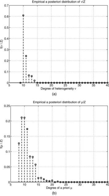
Fig. 4. Empirical posterior distribution of º_{j Z and ¹ j Z.} KA-heterogeneous model. º = 10, ¹ = 10, K = 24, ¹_min= 9,

¹_max= 40.

Markov chains have to be run independently with assumed values for N_bi and N_r. The appropriate values of N_bi and N_r have to be chosen in order to provide an adequate potential scale reduction factor. In our case, the convergence was assessed for N_bi= 100 and N_r= 2000 (for more details on the procedure, the reader is invited to consult the analysis conducted in [39]). We stress that the values of N_bi and N_r are high and impact the computational load accordingly. But as we see later for a STAP scenario, the method, though computationally intensive, brings undeniable advantages.

Once the algorithm parameters are set to adequate values, the performance of the estimators (12) can be studied. Fig. 4 displays the empirical posterior distributions of º_{j Z and ¹ j Z for a highly} heterogeneous scenario (º = 10) with inaccurate a priori (¹ = 10). The estimated posteriors are

Fig. 5. MSE for parameter M_p. KA-heterogeneous model. ¹ = 20, K = 24, ¹_min= 9, ¹_max= 40.

Fig. 6. Theoretical posterior distribution of ¹j Z. KA-homogenous model. K = 24, ¹_min= 9, ¹_max= 40.

consistent with the true values of º and ¹. Fig. 5 shows the MSE for the parameter M_p as a function of º. Three estimators of M_p are compared: the MMSE estimator (12), the MMSE estimator when º and ¹ are known [38], and also the SCM. The two MMSE estimators outperform the SCM significantly, especially when the environment is highly heterogeneous (small º). We also observe that the robustified algorithm of Section II incurs small losses compared with its first version [38] that assumed known values of º and ¹.

2) KA-Homogeneous Model: This section studies the estimators (30) and (37) derived under the assumption of a KA-homogenous model. Data are generated according to (21) and (22). For comparison purposes, we set the bounds for the estimation of ¹ to ¹_m= ³ + 1 and ¹_M = 5³. The posterior distribution

Fig. 7. MSE for parameter M_p. KA-homogeneous model. K = 24, ¹_min= 9, ¹_max= 40.

f(¹_{j Z) is depicted in Fig. 6. As can be seen, the pdf} is very sharp for small ¹ but gets wider for larger ¹. Fig. 7 displays the MSE for the parameter M_p as a function of the degree of a priori knowledge ¹. Three estimators are compared: the MMSE estimator (37), the MMSE estimator (37) with known ¹ (i.e., the method of [36]), and the SCM. The robust estimator (37) performs almost as well as the MMSE estimator with known ¹. When the degree of a priori is small (¹_{¼ ³ + 1), the MMSE estimator performs similarly to} the SCM. Indeed, for small ¹, ¯M_p does not provide additional information on the primary covariance matrix M_p, and the traditional and less complex SCM can be used instead. Yet when ¹ increases, the MSE of the MMSE estimator decreases, while that of the SCM remains constant. Thus, the MMSE estimator (37) takes advantage of both the homogeneous data and the prior information.

B. Synthetic STAP Data

1) Scenario Parameters: In this section, we consider an airborne radar sending a burst of M chirps at the pulse repetition frequency (PRF) f_r. The carrier frequency is denoted by f₀. The antenna is a uniform linear array (ULA) with N half-wavelength inter-spaced elements. We focus our attention on a scenario exempt from jammers. The target-free space-time snapshot z_j at the jth range gate is

generated as a centered complex Gaussian vector with covariance matrix M_j, i.e.,

z_{j» ˜N³}(0, M_j):

Thermal noise and ground clutter are assumed to be independent; thereby

M_j= M_c,j+ M_n (40)

where

M_nis the thermal noise covariance matrix. Assuming a mutual independence between channels and under the ULA assumption, M_n= ¾2I with ¾2_the noise power per element.

M_c,j is the clutter covariance matrix at the jth gate generated according to the GCM described in [1]. Succinctly, it is defined as the integral of independent clutter sources evenly distributed in azimuth

M_c,j= ¾2 Na X r=1 Np X p=1 »_p,r;jf¡p,r;j− INg ¯ fa(p,r;j)a(p,r;j) H g (41) where

− is the Kronecker matrix operator, ¯ is the Hadamard matrix operator, N_a is the number of range ambiguities, N_p is the number of ground patches,

»_p,r;j is the clutter-to-noise ratio associated with the (p, r)th patch at the jth range gate and is obtained from the radar equation as in [1, p. 23],

¡_p,r;j is the intrinsic clutter motion (ICM)

covariance matrix for the (p, r)th patch at the jth range gate,

a(p, r; j) is the space-time steering vector associated

with the (p, r)th patch at the jth range gate. The ICM stands for the pulse-to-pulse fluctuation of the clutter amplitude. In the following, the ICM is assumed to be independent of the clutter patch number, and it is modeled with a Gaussian spectrum [46], i.e., ¡_p,r;j= Toeplitz_f°c(0), : : : , °_c(M_{¡ 1)g} with °_c(m) = exp ( ¡1₂ μ 4¼¾_vf0 cf_rm ¶2) ₍₄₂₎

where c is the propagation velocity and ¾_v is the velocity standard deviation. The space-time steering vector a(p, r; j) can be expressed as the following Kronecker product:

a(p, r; j) = a_t(p, r; j)_{− as}(p, r; j) where a_t(p, r; j) and a_s(p, r; j) are, respectively, the M-length temporal steering vector and the N-length spatial steering vector associated with the (p, r)th patch at the jth range gate, i.e., for m = 0, : : : , M_{¡ 1} and n = 0, : : : , N_{¡ 1,} [at(p, r; j)]m= exp μ j2¼m2v c f₀ fr cos(μ_p,r;j) sin(Á_p,r;j+ Áa) ¶ [a_s(p, r; j)]_n= exp μ j2¼nd ¸₀cos(μp,r;j) sin(Áp,r;j) ¶ where

d is the interelement distance, ¸₀= c=f₀ is the wavelength, v is the radar platform velocity,

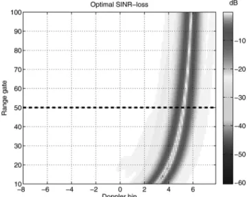
Fig. 8. Range-Doppler map: optimal SINR-loss. TABLE I Scenario Parameters Parameter Value velocity v = 100 m/s crab Á_a= 90± carrier f₀= 450 MHz PRF f_r= 750 Hz pulses M = 16 channel N = 8 interelement distance d = ¸₀=2

element pattern cosine

backlobe level b_e=¡30 dB CNR1(range #1) CNR = 40 dB

ICM ¾_v= 0:25 m/s

Note: 1_{Clutter-to-noise ratio.}

(Á_p,r;j, μ_p,r;j) is the azimuth and depression angle of the (p, r)th clutter patch at the jth range gate,

Á_a is the misalignment angle between the velocity vector and the lengthwise direction of the ULA. Hereafter, we assume a scenario without range ambiguities, i.e., N_a= 1. A forward-looking antenna (i.e., Á_a= 90±) is considered to obtain a nonstationary clutter [1, 2]. Such geometrical configuration ensures, indeed, that the spatio-Doppler frequencies occupied by the clutter vary over range as depicted in Fig. 8 (the SINR loss is defined later). We focus the analysis on the range gate 50 where the clutter is highly nonstationary. Scenario parameters useful to generate

M_c,j according to (41) are given in Table I. 2) Processing Parameters: We apply the estimation procedures within a reduced-dimension algorithm with a post-Doppler structure. Indeed, it allows one to apply the estimation procedure locally over M0_{¿ M Doppler bins. Moreover, it significantly} decreases the computational load. More precisely, an extended factored algorithm (EFA) has been chosen with M0= 3 Doppler bins and without zero-padding

[1, 47]. Thus, for a given range gate, the estimation procedure is applied M times (one time per bin) with ³ = NM0= 24.

Only one prior matrix ¯M_p of dimension NM_{£ NM} is generated and then projected onto the appropriate reduced Doppler-element domain. The a priori

covariance matrix is built in a similar way to (40), i.e., ¯

M_p= ¯M_n+ ¯M_c,50 (43) where ¯M_n and ¯M_c,50 are the noise and clutter

components, respectively. The noise component ¯M_n

is supposed to be known exactly, i.e., ¯M_n= M_n. The clutter component ¯M_c,50 is built upon the GCM model according to (41) but departs from the true matrix

M_c,50. Indeed, three parameters of the GCM have been changed as follows:

1) the ICM has been overestimated with the value ¾_v= 0:5 m/s,

2) a misalignment of ¢Á_a= 2± has been introduced between the velocity vector and the longitudinal axis of the fuselage,

3) the backlobe level of the element pattern has been increased to b_e=_{¡5 dB.}

The first two modifications represent errors that are common in real scenarios. Although the third modification is less realistic, its impact is localized in the Doppler domain and hence, as shown later, it allows us to illustrate the performance of our algorithms in a case where the environment is homogeneous and the a priori highly inaccurate. Finally, the number of secondary data is set to K = 2³ = 48. The bounds for hyperparameter estimation are set to

º_m= ³ + 1 = 25, ¹_m= ³ = 24, º_M = ¹_M = 5³ = 120 for the KA-heterogenous model,

¹_m= ³ + 1 = 25, ¹_M= 5³ = 120 for the KA-homogeneous model.

3) Results: We observe in this section the STAP filter shape for different estimates ˆM_p of the noise covariance matrix. To do so, we display the SINR loss defined as [2] L = jw H_a j2 wH_M pw 1 aH_M¡1 n a (44) where a is the steering vector and w_{/ ˆ}M¡1

p a is the STAP filter. Results are averaged using M_c= 100 Monte Carlo runs. Additionally for each Doppler bin, we observe the average values of the hyperparameters º and ¹ as well as the average values of the weighting factors w and ¯w, given by (38). Results are displayed in Fig. 9.

Before analyzing the behavior of the MMSE estimators, we recall first that the optimal filter in an EFA structure is obtained by the clairvoyant case, i.e., ˆM_p= M_p. Note also the expected behavior of the SCM filter that performs badly around the clutter

Fig. 9. KA-estimation assuming homogenous environment: SINR loss (a), estimated ¹ (c), weights w and ¯w (e). KA-estimation assuming heterogeneous environment: SINR loss (b), estimated ¹ (d), estimated º (f).

notch (fifth Doppler bin), as the clutter is highly nonstationary. Elsewhere, the SCM filter incurs a 3dB loss (compared with the optimal filtering in an

EFA structure) as predicted by the Reed, Mallett, and Brennan rule [5]. Finally, we emphasize that the forward-looking scenario and the a priori matrix have

TABLE II

Distinct Domains of Environment and a priori

Domain Bins Environment a priori

D1 f¡8,¡7g \ f¡3,:::,2g homogeneous accurate

D2 f¡6,:::,¡4g homogeneous inaccurate

D3 f3,:::,6g heterogeneous accurate

been chosen so that three different areas can be clearly identified, as summarized in Table II:

1) Observing Fig. 8 and according to the training interval, it is clear that the clutter is highly nonstationary from bin 3 to 6. Elsewhere the

secondary data are homogenous with the primary one. 2) Observing now the filter shape of the prior matrix in Fig. 9, one can see that the a priori information is rather accurate except from bin_¡6 to_{¡4. A slight ICM overestimation (as suggested} in [21]) and a small crab error do not significantly affect the mainlobe clutter notch other than a slight widening and deepening. Note also that the backlobe level, which has been increased to build ¯M_p, impacts only bin_{¡6 to ¡4.}

Of course, some specific algorithms (e.g., the extended sample matrix inversion [48]) are efficient at counteracting the nonstationarity of the clutter considered here (especially when the nonstationarity is so continuous). However, the simplicity of the scenario allows us to characterize at once the behavior of the studied estimators for three distinct cases as described in Table II. The contrast is not so distinct with more realistic clutter. In the following, we comment on Figs. 9 and 10, which depict the performance of the MMSE estimators of Sections II and III and also, for comparison purposes, the CL estimator presented in [32].

Observing Figs. 9(a), (c), and (e), the following comments can be made on the MMSE estimators based on a KA-homogeneous model.

1) The filter built with the estimator (37) does not perform well in the nonstationary domain_D3or in_D2 where the a priori information is not accurate. Close to optimal performance is observed in domain_D1 where the environment is actually homogeneous and the a priori matrix is accurate.

2) The estimated degree of a priori ¹ (30) is large in the domain_D1 but has small values elsewhere in D2and _D3. Thus, the estimator fails at recognizing the domain_D3. Note that ¹ is closely related to the weight

¯

w of the a priori matrix.

This behavior can be explained as follows. 1) In domain_D3, the data do not respect the homogeneous assumption used to derive (30) and (37). This leads to underestimation of ¹ and ¯w. Thus

the estimator (37) does not give enough weight to the a priori matrix.

2) In domain_D2, the estimation of ¹ seems adequate because the a priori information is not accurate. However, the filter based on (37) does not perform much better than the a priori filter. Indeed the weight ¯w, though small ( ¯w_{¿ 1), is not equal to} zero, and thus the a priori matrix cannot be totally rejected in the estimate. In other words, the number of secondary data K is not large enough so that the SCM outweights the prior matrix. This behavior is very undesirable and contrasts the results obtained for the MSE of M_p(37) when the data are generated according to the KA-homogenous model.

The performance of the MMSE estimators based on the assumption of a KA-heterogeneous model are depicted in Figs. 9(b), (d), and (f). The following points can be underlined.

1) The proposed filter always provides the best performance among the three adaptive filters under study. It behaves like the a priori filter in_D1 and_D3 when the later outperforms the SCM filter. Otherwise, the filter behaves like the SCM filter.

2) The values of the estimated ¹ are large in D1and_D3, i.e., ˆ¹mmse_{¼ ¹M, when the a priori} information is accurate. In domain_D2, where the a priori is not precise, the estimated values of º are low, i.e., ˆ¹mmse_{¼ ¹m}. Thus the estimate of ¹ identifies correctly and precisely whether the a priori information is reliable or not.

3) The estimated values of the degree of heterogeneity º are more contrasted. In domain _D2, the values of º are small ( ˆºmmse_{¼ ºm). ThusD2is} correctly identified as a nonhomogenous environment. In domains_D1and_D3, the values of º are large but endure some variations, though the environment is equally homogeneous over the area. Especially around the fourth Doppler bin, the value of º decreases where the degree of a priori is small.

Thus the estimate of ¹ is a very important quantity. It defines the shape of the filter: if ¹ is large the filter behaves like the a priori filter; if ¹ is small the filter behaves like the SCM filter. It also correctly identifies if the a priori matrix brings an accurate information and incorporates or discards it accordingly in the covariance matrix estimate. As expected the heterogenous model (3) is perfectible. Indeed the filter does not outperform the SCM filter if the prior matrix is not accurate. However, the model (3) gives some kind of degree of freedom between the prior knowledge and the secondary data that allows one an appropriate incorporation of the prior matrix. Moreover, the estimate of º provides additional information. It identifies correctly the heterogeneity

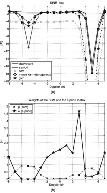
Fig. 10. GLC-CL estimation: SINR loss (a), weights ® and ¯ (b).

as long as the prior is accurate enough (otherwise the algorithm seems to suffer from a lack of reference).

The behaviors of the two estimation procedures are summarized in Table III. Of course the Gibbs sampling strategy is highly computationally intensive. Moreover, the interpretation of its estimators is made harder because they are not obtained in closed form (12). However, unlike the estimation based on a KA-homogenous model, the algorithm is able to identify precisely the accuracy of the prior matrix whether the environment is heterogeneous or not. Furthermore, the matrix estimate derived under the heterogeneous assumption can entirely reject the a priori matrix, which is a desirable property, especially when this matrix does not bring trustworthy information. In light of these results, it is clear

that using the heterogeneity relation (3) of the KA-heterogeneous model is actually relevant.

TABLE III

Summary of the Performance of the MMSE Estimates on STAP Synthetic Data

Environment a priori a priori Identification º Identification ¹ Incorporation KA-H1 _KA-NH2 _{KA-H KA-NH KA-H KA-NH}

Data Type D1 Ø p p p p p D2 Ø ¼ p p £ p D3 Ø p £ p £ p

Note: 1,2_{KA-homogenous model, KA-heterogeneous model. Ø,}

¼, p,£ none, approximate, correct, not correct.

Finally, before closing this section, the two Bayesian approaches are compared with the

deterministic CL technique presented recently in [32]. More precisely, we have considered the general linear combination (GLC) technique. The covariance matrix estimate is supposed to be a linear combination of the SCM and the prior matrix

ˆ

Mglc_p = ¯ ˆMscm_p + ® ¯M_p (45) with ® > 0 and ¯ > 0. The weighting factors ® and ¯ are then derived so as to minimize the MSE between

ˆ

Mglc

p and the clairvoyant covariance matrix Mp. More precisely, as M_p is not known a priori, an estimate of the MSE is considered instead. The latest is obtained, assuming that the SCM is unbiased. Fig. 10 displays the STAP filter shape and the GLC00 weighting factors.

1) In domain_D1 and_D3, the GLC filter behaves like the filter based on the KA-homogenous model. Near-optimal performance is obtained in _D1 where the environment is homogeneous and the prior matrix is accurate. In_D3, the heterogeneity prevents an appropriate estimation of the weighting factors.

2) Interestingly, in domain_D2, the GLC method is able to reject almost entirely the prior information that is unprecise.

Thus the deterministic CL estimate (45) performs better than the Bayesian CL estimate (37). However, the Bayesian CL technique is able to identify the degree of a priori when the environment is homogeneous. This information is not provided as clearly by the GLC technique. In any event, the Bayesian estimators, based on the assumption of a KA-heterogenous model, provide better filtering and also important information regarding the degrees of a priori and heterogeneity.

V. CONCLUSIONS

In KA-STAP, a priori information is used to improve the detection performance in highly heterogeneous environments. In this context, we have presented two estimation schemes designed to incorporate a prior matrix in the noise covariance matrix estimate. Both schemes rely on Bayesian

data models. The first model also entails an original relation of heterogeneity that describes how the secondary covariance matrix differs from the primary one. The second model assumes a

homogenous environment. The KA part and (possibly) the heterogeneity relation of the models involve hyperparameters that represent the degrees of a priori and heterogeneity, respectively. The MMSE estimators of both the hyperparameters and the covariance matrix are derived. For the KA-heterogeneous model, the estimation is performed via a Gibbs sampling strategy that is highly computationally intensive. For the KA-homogenous model, the MMSE estimators are obtained in closed form, and the algorithm turns out to belong to the well-known CL technique. Performance analysis on STAP synthetic data shows that it is essential to take into account the heterogeneity in the data model. It brings a degree of freedom between the secondary data and the prior matrix that allows one to identify and incorporate the prior information in an appropriate way. Otherwise the proposed estimators are not able to reject inaccurate information, yet achievable with a less complex deterministic CL method. Additionally, the estimation scheme based on the first model yields precise information on the degree of heterogeneity if the prior information is accurate. Finally, one can think of some refinements for the future. As expected, the heterogenous model might be improved. Indeed when the a priori information is not reliable, the KA-STAP filter does not perform better than the SCM filter. Also the computational load induced by the MCMC method is currently a drawback for real-time processing.

REFERENCES [1] Ward, J.

Space-time adaptive processing for airborne radar. Lincoln Laboratory, MIT, Lexington, MA, Technical Report 1015, Dec. 1994.

[2] Klemm, R.

Principles of Space-Time Adaptive Processing.

London: IEE Press, 2002. [3] Guerci, J. R.

Space-Time Adaptive Processing for Radar.

Norwood, MA: Artech House, 2003. [4] Brennan, L. E. and Reed, I. S.

Theory of adaptive radar.

IEEE Transactions on Aerospace and Electronic Systems, 9,

2 (Mar. 1973), 237—252.

[5] Reed, I. S., Mallett, J. D., and Brennan, L. E. Rapid convergence rate in adaptive arrays.

IEEE Transactions on Aerospace and Electronic Systems,

AES-10, 6 (Nov. 1974), 853—863.

[6] Melvin, W. L.

STAP in heterogeneous clutter environments.

In R. Klemm, (Ed.), Applications of Space-Time Adaptive

Processing, 2004, ch. 10, 305—358.

[7] McDonald, K. F. and Blum, R. S.

Robust techniques in space-time adaptive processing. In R. Klemm, (Ed.), Applications of Space-Time Adaptive

Processing, 2004, ch. 13, 413—461.

[8] Melvin, W. L.

Space-time adaptive radar performance in heterogeneous clutter.

IEEE Transactions on Aerospace and Electronic Systems,

36, 2 (Apr. 2000), 621—633.

[9] Guerci, J. R., Goldstein, J. S., and Reed, I. S. Optimal and adaptive reduced-rank STAP.

IEEE Transactions on Aerospace and Electronic Systems,

36, 2 (Apr. 2000), 647—663.

[10] Carlson, B. D.

Covariance matrix estimation errors and diagonal loading in adaptive arrays.

IEEE Transactions on Aerospace and Electronic Systems,

24, 4 (July 1988), 397—401.

[11] Steiner, M. and Gerlach, K.

Fast converging adaptive processor for a structured covariance matrix.

IEEE Transactions on Aerospace and Electronic Systems,

36, 4 (Oct. 2000), 1115—1126.

[12] Fuhrmann, D. R.

Application of Toeplitz estimation to adaptive beamforming and detection.

IEEE Transactions on Signal Processing, 39, 10 (Oct.

1991), 2194—2198.

[13] Rabideau, D. J. and Steinhardt, A. O.

Improved adaptive clutter cancellation through data-adaptive training.

IEEE Transactions on Aerospace and Electronic Systems,

35, 3 (July 1999), 879—891.

[14] Chen, P., Melvin, W. L., and Wicks, M. C. Screening among multivariate normal data.

Journal of Multivariate Analysis, 69, 1 (Apr. 1999), 10—29.

[15] Scharf, L. L. and McWhorter, L. T.

Adaptive matched subspace detectors and adaptive coherence estimators.

In Proceedings of the 30th Asilomar Conference on Signals,

Systems, and Computers, Pacific Grove, CA, Nov. 1996,

1114—1117. [16] Pascal, F., et al.

Covariance structure maximum-likelihood estimates in compound Gaussian noise: Existence and algorithm analysis.

IEEE Transactions on Signal Processing, 56, 1 (Jan. 2008),

34—48.

[17] Gini, F. and Rangaswamy, M.

Knowledge-Based Radar Detection, Tracking and Classification.

Malden, MA: Wiley InterScience, 2008.

[18] Gini, F., Goldstein, J. S. and Zoltowski, M. D. (Eds.) Knowledge-based systems for adaptive radar: Detection, tracking and classification.

IEEE Signal Processing Magazine, 23, 1 (Jan. 2006),

special section.

[19] Proceedings KASSPER Workshops, 2002—2005 [Online], formerly available:

http://www.darpa.mil/sto/space/kassper.html (accessed Mar. 2008).

[20] Guerci, J. R. and Baranoski, E. J.

Knowledge-aided adaptive radar at DARPA.

IEEE Signal Processing Magazine, 23, 1 (Jan. 2006),

41—50.

[21] Melvin, W. L. and Guerci, J. R.

Knowledge-aided signal processing: A new paradigm for radar and other advanced sensors.

IEEE Transactions on Aerospace and Electronic Systems,

42, 3 (July 2006), 983—996.

[22] Capraro, C. T., et al.

Implementing digital terrain data in knowledge-aided space-time adaptive processing.

IEEE Transactions on Aerospace and Electronic Systems,

[23] Conte, E., et al.

Design and analysis of a knowledge-aided radar detector for Doppler processing.

IEEE Transactions on Aerospace and Electronic Systems,

42, 3 (July 2006), 1058—1079.

[24] Gerlach, K. and Picciolo, M. L.

Airborne/spacebased radar STAP using a structured covariance matrix.

IEEE Transactions on Aerospace and Electronic Systems,

39, 1 (Jan. 2003), 269—281.

[25] Melvin, W. L. and Showman, G. A.

An approach to knowledge-aided covariance estimation.

IEEE Transactions on Aerospace and Electronic Systems,

42, 3 (July 2006), 1021—1042.

[26] Hiemstra, J. D.

Colored diagonal loading.

In Proceedings of the IEEE Radar Conference, Chantilly, VA, Apr. 22—25, 2002, 386—390.

[27] Teixeira, C., Bergin, J., and Techau, P.

Reduced degree-of-freedom STAP with knowledge-aided data pre-whitening.

In Proceedings of KASSPER Workshops 2003, Las Vegas, NV, Apr. 2003.

[28] Bergin, J. S., et al.

STAP with knowledge-aided data pre-whitening. In Proceedings of the IEEE Radar Conference, Philadelphia, PA, Apr. 26—29, 2004, 289—294. [29] Page, D., et al.

Improving knowledge-aided STAP performance using past CPI data.

In Proceedings of the IEEE Radar Conference, Apr. 26—29, 2004, 295—300.

[30] Blunt, S. D., Gerlach, K., and Rangaswamy, M. STAP using knowledge-aided covariance matrix estimation and the FRACTA algorithm.

IEEE Transactions on Aerospace and Electronic Systems,

42, 3 (July 2006), 1043—1057.

[31] Zhu, X., et al.

Knowledge-aided space-time adaptive processing. In Proceedings of the 41st Asilomar Conference, Pacific Grove, CA, Nov. 4—7, 2007, 1830—1834.

[32] Stoica, P., et al.

On using a priori knowledge in space-time adaptive processing.

IEEE Transactions on Signal Processing, 56, 6 (June

2008), 2598—2602.

[33] Besson, O., Bidon, S., and Tourneret, J-Y.

Covariance matrix estimation with heterogeneous samples.

IEEE Transactions Signal Processing, 56, 3 (Mar. 2008),

909—920. [34] Bergin, J., et al.

Space-time beamforming with knowledge-aided constraints.

In Proceedings of the Adaptive Sensor Array Processing

Workshop, Mar. 11—13, 2003.

[35] Besson, O., Tourneret, J-Y., and Bidon, S.

Knowledge-aided Bayesian detection in heterogeneous environments.

IEEE Signal Processing Letters, 14, 5 (May 2007),

355—358.

[36] De Maio, A. and Farina, A.

Adaptive radar detection: A Bayesian approach. In Proceedings of the 2006 International Radar

Symposium, Krakow, Poland, May 24—26, 2006.

[37] De Maio, A., Farina, A., and Foglia, G.

Adaptive radar detection: A Bayesian approach. In Proceedings of the IEEE Radar Conference, Waltham, MA, Apr. 17—20, 2007, 624—629.

[38] Bidon, S., Besson, O., and Tourneret, J-Y. A Bayesian approach to adaptive detection in nonhomogeneous environments.

IEEE Transactions on Signal Processing, 56, 1 (Jan. 2008),

205—217.

[39] Bidon, S., Besson, O., and Tourneret, J-Y.

Characterization of clutter heterogeneity and estimation of its covariance matrix.

In Proceedings of the 2008 IEEE Radar Conference, Rome, Italy, May 26—30, 2008, 357—362.

[40] Gelman, A., et al.

Bayesian Data Analysis (2nd ed.).

New York: Chapman & Hall, 2004. [41] Anderson, T. W.

An Introduction to Multivariate Statistical Analysis (2nd

ed.).

Hoboken, NJ: Wiley, 1984. [42] Earp, S. L. and Nolte, L. W.

Multichannel adaptive array processing for optimal detection.

In Proceedings of the International Conference on

Acoustics, Speech, and Signal Processing (ICASSP), vol.

1, San Diego, CA, Mar. 1984, 267—270. [43] Robert, C. P.

The Bayesian Choice, From Decision-Theoretic Foundations to Computational Implementation.

New York: Springer, 2007. [44] Robert, C. P. and Casella, G.

Monte Carlo Statistical Methods (Springer Texts in

Statistics).

New York: Springer, 2004. [45] Robert, C. P.

Discretization and MCMC Convergence Assessment.

Berlin: Springer-Verlag, 1998. [46] Barton, D. K.

Radar Clutter.

Norwood, MA: Artech House, 1975. [47] DiPietro, R. C.

Extended factored space-time processing for airborne radar systems.

In Proceedings of the 26th Asilomar Conference on Signals,

Systems, and Computers, vol. 1, Pacific Grove, CA, Oct.

26—28, 1992, 425—430. [48] Hayward, S. D.

Adaptive beamforming for rapidly moving arrays. In Proceedings of the International Conference on Radar, Beijing, China, Oct. 8—10, 1996, 480—483.