Impact of SOC variations on the battery bank sizing of a stand-alone system fed by a passive wind turbine

Open Archive TOULOUSE Archive Ouverte (OATAO)

OATAO is an open access repository that collects the work of Toulouse researchers and

makes it freely available over the web where possible.

This is an author-deposited version published in :

http://oatao.univ-toulouse.fr/

Eprints ID : 12206

To cite this version :

Belouda, Malek and Sareni, Bruno and

Roboam, Xavier and Belhadj, Jamel Impact of SOC variations on

the battery bank sizing of a stand-alone system fed by a passive

wind turbine. (2014) International Journal of Renewable Energy

Research, vol. 4 (n° 3). pp. 555-565. ISSN 1309-0127

Any correspondance concerning this service should be sent to the repository

administrator:

[email protected]

Impact of Soc Variations on the Battery Bank Sizing

of a Stand-Alone System Fed by a Passive Wind

Turbine

Malek BELOUDA*, Bruno SARENI**, Xavier ROBOAM** Jamel BELHADJ*

*University of Tunis El Manar, ENIT, L.S.E, B.P. 37, 1002, Tunis le Belvédère-Tunisie

**University of Toulouse, LAPLACE UMR CNRS–INP–UPS, ENSEEIHT 2, Rue Ch Camichel 31071 Toulouse – France

([email protected], [email protected], [email protected], [email protected])

‡  _{Corresponding Author; Malek BELOUDA, ENIT, L.S.E, B.P. 37, 1002, Tunis le Belvédère-Tunisie, Tel: +216 71 874 700,} Fax: +216 71 872 729

Abstract- This study compares and analyses two passive wind turbine system models in order to show their equivalence

through a storage bank sizing procedures. The main differences between both models reside in the design accuracy and the computational time needed for each model to simulate the wind turbine system behaviour. On the one hand, a first “mixed reduced model” neglects the electrical mode effect and assumes that the DC battery bus voltage is constant (i.e. invariable State Of Charge: SOC). On the other hand, the second “full analytic model” couples SOC fluctuations (i.e. bus voltage variations) in the whole system. When compared to the second model, the “mixed reduced model” allows reducing computational time, which is a major factor in the context of systemic design by optimization. The analysis is performed to put in evidence the correspondence between both sizing approaches with the two corresponding models. The results are finally discussed from the viewpoint of the compromise design accuracy and computational time reduction. In this paper, the authors compare and analyse two passive wind turbine system models in order to show their equivalence through a storage bank sizing procedures. The main differences between both models reside in the design accuracy and the computational time needed for each model to simulate the wind turbine system behaviour. On the one hand, a first “mixed reduced model” neglects the electrical mode effect and assumes that the DC battery bus voltage is constant (i.e. invariable State Of Charge: SOC). On the other hand, the second “full analytic model” couples SOC fluctuations (i.e. bus voltage variations) in the whole system. When compared to the second model, the “mixed reduced model” allows reducing computational time, which is a major factor in the context of systemic design by optimization. The analysis is performed to put in evidence the correspondence between both sizing approaches with the two corresponding models. The results are finally discussed from the viewpoint of the compromise design accuracy and computational time reduction. Do not use abbreviations in the title unless they are unavoidable.

Keywords Energy storage, passive wind turbine, battery sizing, mixed reduced model, full analytic model, SOC variations.

1. Introduction

Currently, hybrid (PV – wind) systems with several means of storage (accumulators, H2 storage, etc) and sometimes with available energy sources (Diesel generator, fuel cells) are widely used mainly for isolated areas, especially for electricity production, water pumping and desalination. Designing these complex systems through an optimization design approach requires simulating well

adapted models to characterize their behaviour and efficiency [1-3]. Generally, the use of high accurate models would lead to a “perfect system design”, but such an approach suffers from the quite high computational time needed by model processing: the granularity (accuracy/complexity) versus computation time is then a crucial trade-off especially for Integrated Optimal Design (IOD) process.

This article then proposes a storage device sizing based on electrochemical accumulators associated to a passive

wind turbine subjected to wind speed variations in order to jointly supply a load demand. Two different models are proposed for processing this sizing: the first one, so called “mixed reduced model” neglects the electrical mode effect but simulates the mechanical one, especially due to the turbine inertia. With this “low cost” model (in terms of computation complexity), we assume that the DC bus voltage (and consequently the battery SOC) is constant. A second model called “full analytic model” also neglects the mechanical mode. Such modelling allows coupling voltage fluctuations of the DC bus, by taking account of SOC variations. Therefore, the use of this model, offering a reduction of computational time and keeping a sufficient accuracy is the more adapted in an optimization design approach if SOC variations have to be considered. However, in such a case, all elements (i.e. wind source, storage device and load demand) are strongly coupled in the system. On the contrary, when the first mixed reduced model is used by neglecting SOC, then voltage variations, the battery bank sizing may be decoupled from source-load association. As it will be analyzed in this paper, only the power difference (source-load) along time impacts the storage sizing in terms of power AND energy.

Numerous wind turbine system architectures can be proposed, especially for reduced power scale applications [4 - 7] but the considered system is a 8 kW full passive wind turbine battery charger without active control and with minimum number of sensors as studied in [7 - 9].The system parameters have been sized by similitude from a 1.7 kW optimized passive wind turbine system [8]. A battery sizing procedure based on both different models are used for linking the wind energy potential with a given load power demand. These approaches are compared to evaluate the ad-equation of each model with the sizing approaches and eventually in an IOD context.

The study is structured as follows. The passive wind system, the wind speed profile and the load demand are described in section 2 which sets the system sizing problem. Both simulating models of the wind turbine system are presented in the third section. Section 4 is dedicated to the battery sizing procedures following the considered model with and without coupling with SOC variations. Section 5 is reserved to exhibit and compare results from the both sizing approaches.

Nomenclature

Ccel Cell capacity (A.h)

Cp Power coefficient

e0 Voltage of cell (V)

EBT Energy storage capacity (Wh)

E Stator electromotive force (V)

Ibat Battery current

Icel Cell current (A)

Iload Load current

Is Stator current (A)

JWT Wind turbine inertia (Kg.m2)

Ls Stator inductance (Ω)

Ncel_p Number of cells in parallel Ncel_s Number of cells in series

Nspp Number of slots per pole per phase

p Pole pair number

PBTAV Average battery power (W)

PBT Battery power (W)

PEddy Eddy current losses (W)

PHyst Hysteresis losses (W)

Pload Load power (W)

Pext Extracted power (W)

PWT Mechanical wind turbine output power (W)

rcel Internal resistance of a cell(Ω)

Rd Diode internal resistance (Ω)

Rs Stator resistance (Ω)

S Swept rotor area (m2₎

Tem Electromagnetic torque (N.m)

TWT Wind turbine torque (N.m)

Ud0 Diode voltage drop (V)

UDC DC bus voltage (V)

v wind speed (m/s)

Vcel Voltage at cell terminals (V)

Vs Stator voltage (V)

ΔSOCk Cell state of charge variation

ΔT Sampling time

λ Tip speed ratio

ρ Air density (kg.m-3)

Φs Stator flux (Wb)

ω Electric pulsation (rd/s)

Ω Wind turbine rotational speed (rd/s)

ΔUDC DC bus voltage variation (V)

2. Passive Wind System Structure And Environmental Variables

2.1. Passive Wind System Structure

In the objective of maximizing reliability and to reducing the system cost, a passive wind turbine with low DC output

voltage (here about 48V) is considered. A battery bank is coupled to the DC bus at the output of a diode bridge rectifier in order to ensure an autonomous system operation for remote applications. This system operates without controlled power devices and by a minimum number of sensors (Error! Reference source not found.) [7].

    Load   de m an d PMSG Battery  bank   Diode  rectifier   Wind  cycle   profile   Turbine   Rotor Stator Optimized PMSG

Fig. 1. Passive wind turbine system subjected to a wind

profile and a load profile.

In [8], an IOD process, founded on multi-objective optimization, has been performed for sizing the elements of a 1.7 kW passive wind turbine system (Error! Reference

source not found. 1). Experimental measurements on a test

bench consisting of a passive wind turbine and a lead-acid battery (48V DC bus), allowed us to characterize the extraction quality of wind power (useful power recovered by this passive structure). Quantitatively, we have shown that it is possible to extract a power of about 90% of the power supplied by an ideal turbine (constantly maintained at optimal regime).

The behaviour of the considered optimized passive wind turbine can match very closely that of active wind turbine systems operating at optimal wind powers by using an MPPT control device (0 2). The corresponding theoretical and experimental PMSG electrical parameters used in the prescribed models are mentioned in 0 1.

Certain characteristics of the passive structure reveal sensitivity to some design parameters variations and mainly to DC bus voltage fluctuations. It is therefore necessary to further analyze this phenomenon. 0 illustrates the differences between the theoretical and experimental load curves. On one side, we note the horizontal shift of measurements and theoretical curve readjusted from the parameters circuit measurements (theoretical curve 2) and from the original theoretical values of parameters (resistance, inductance, flux (theoretical curve 1) on the other side. This reflects the sensitivity to some parameters which one of them (changes of DC bus voltage) will be discussed in more details in this paper.

0. PMSG circuit and equivalent DC model

correspondence. Theoretical value Measurement Stator resistance (Ω) 0.13 0.13 Cyclic Inductance (mH) 1.42 1.43 Stator flux (Wb) 0.22 0.20

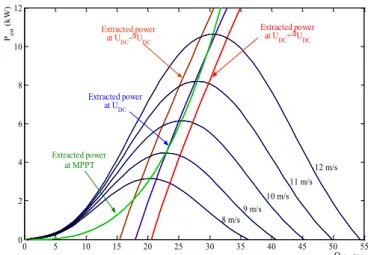
To illustrate the problem of the impact of the change in the battery SOC, and consequently of the DC bus voltage on

the energy efficiency of the passive wind system, 0 shows the load curves of the generator following the value of DC

bus voltage UDC on (here we consider a variation

ΔUDC = ±12% of the nominal value UDC = 48V). The quality

of the power extraction from this passive structure has to be compared with the optimal cubic curve (that could be drawn with MPPT) represented with dotted line on this same graph.

The impact of DC bus voltage fluctuations on the load curve from the curve of the reference generator (curve with the optimal extraction for this passive structure) is well marked. Thus, the passive behaviour of the wind turbine can be modified (improved or degraded) at low and high wind speeds, following the (i.e. SOC) variations.

In this study, a simplified approach has been used based by exploiting similitude effects to rescale the system for higher powers. Hence, using a similitude-based approach, the wind turbine as well as the PMSG features can be deduced for a 8 kW passive wind turbine system [9]

0 500 1000 1500 2000 2500 0 20 40 60 80 100 120

Vitesse de rotation (rad/s)

Ex traction d e p uiss a nc e [W ] Théorique 1 Théorique 2 Points de mesure Vv=8m/s V_v=10m/s V_v=12m/s 0 500 1000 1500 2000 2500 0 20 40 60 80 100 120

Vitesse de rotation (rad/s)

Ex traction d e p uiss a nc e [W ] Théorique 1 Théorique 2 Points de mesure Vv=8m/s V_v=10m/s V_v=12m/s Theoretical curve 1 Theoretical curve 2 Experimental points 0 20 40 60 80 100 120 0.5 1 1.5 2 2.5

Wind turbine rotational speed (rd/s)

Extracted po wer (kW) v=12 m/s v=10 m/s v= 8m/s 0

Fig. 2. Comparison between ideal, theoretical and

experimental load curves.

0 5 10 15 20 25 30 35 40 45 50 55 0 2 4 6 8 10 12 Ω (rad/s) Pex t ( k W) Extracted power at MPPT Extracted power at U_DC Extracted power at U_DC-ΔU_DC Extracted power at U_DC+ΔU_DC 8 m/s 10 m/s 9 m/s 11 m/s 12 m/s

Fig. 3. Impact of DC bus voltage changes on the wind

turbine extracted power. 2.2. Environmental Variables

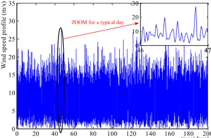
A wind speed profile of 200 days duration is presented in 0. Note that the wind speed profile is obtained from a statistical distribution model (based on Weibull law) from the wind energy potential at a specific location [9]

.

The load profile on one day duration of a typical farm, considered as a case study, is illustrated in 0. The load demand peaks occur between 7 and 8 am and 6 and 9 pm. This day-cycle is repeated along time with regard to wind power variations in order to synthesize the battery power.

3. Passive Wind System Model

In this section, two models are considered. The first is used for simulating the passive wind system in the battery sizing procedure and in which we consider that DC bus voltage is constant and equal to 48 V. While, in the second we will take account of the DC bus voltage variation versus the SOC of the battery bank.

3.1. Wind Turbine Model

The mechanical wind turbine output power, PWT is defined as follows: 3

2

1

Sv

C

P

_WT

=

_p

ρ

(1) Where Cp is the power coefficient corresponding to the turbine studied in [8] (obtained from manufacturer data) and that can be represented with the equation below:

λ

λ

λ

λ

)

0

.

002

.

0

.

021

0

.

013

.

(

=

−

3

+

2

+

p

C

(2)

Where λ is the tip speed ratio: v RΩ =

λ

.

3.2. Modelling of the PMSG – Rectifier Association

The DC equivalent-reduced model is a simplified model of the PMSG associated with a diode bridge rectifier considering the diode overlapping during switching intervals. This model is used in the battery sizing process for the simulation of the passive wind turbine system.

0 20 40 60 80 100 120 140 160 180 200 0 5 10 15 20 25 30 35 time(days) Wi nd s pe ed p ro fi le ( m /s ) 46 4747 0 10 20 30 ZOOM for a typical day

Fig. 4. Wind speed profile.

6 0 time(h) 3 6 9 12 15 18 21 24 0 1 2 3 4 5 PLoad/day (kW)

Fig. 5. The farm load mission for one day.

3.3. Equivalent DC Model

The simplified causal model represents the PMSG-rectifier association with a DC model energetically equivalent in terms of average values. This PMSG equivalent circuit model is given in 0.

0 illustrates the synoptic of the equivalent DC model where causality is symbolized by arrows specifying which physical variables (energetic flows or efforts) are applied to each part of the system. The correspondence between AC (rms) values and DC ones, in the PMSG circuit model, is shown in Error! Reference source not found..

3.4. Equivalent DC Electromechanical Model

The electromechanical conversion is modelled by the following equation:

⎩

⎨

⎧

Ω

Φ

=

Φ

=

.

'

DC sDC sDC DC em

p

E

I

p

T

(3)   Vs Es RS LS IS E’s

Fig. 6.The PMSG equivalent circuit.

 

_Ω

T

em E’SDC SDC Electromechanic Conversion (Voltage source) Armature reaction (Voltage drop) Transient electric mode (Power loss) Commutation Interval in the Diode Rectifier (Voltage drop) ESDC I’SDC ISDC EDC ISDC UDC IDC E’SDC SDC ISDC

0. PMSG circuit and equivalent DC model

correspondence.

Variable PMSG Equivalent DC model

Voltage Vs s DC V U = ⋅ π 6 3 Current Is s DC I I = ⋅ 6

π

Flux Φs eff DC = Φ Φ π 6 3 Inductance Ls s DC L L 2 6 3 3 _⎟⎟ ⎠ ⎞ ⎜ ⎜ ⎝ ⎛ = π Resistance Rs s DC R R 2 6 3 3 _⎟⎟ ⎠ ⎞ ⎜ ⎜ ⎝ ⎛ = π Electromotive force Es s sDC E E

π

6 3 =

The armature reaction in the PMSG is represented with a voltage drop without power losses:

(

)

⎪

⎩

⎪

⎨

⎧

=

⋅

⋅

−

=

sDC sDC sDC sDC DC DC DC s sDC

E

I

E

I

s

I

L

E

E

.

'

'

' 2 2

_ω

;

ω= .pΩ (4)

For both reduced models (“mixed reduced” and “full analytic” models), the electric mode effect is neglected, considering that it has a small influence on the energy efficiency issue. It leads to a DC current in the generator defined as: DC sDC sDC DC sDC DC

R

I

E

E

dt

dI

L

+

=

'

−

=> _RDCIsDC=EsDC' _{−EDC (5)}

Diode overlapping during commutation intervals is modelled by a power conservative voltage drop:

⎩

⎨

⎧

=

−

=

DC sDC DC DC DC ov DC DC

U

I

E

I

I

R

E

U

/

; Rov

π

Ls

ω

3 = (6) 3.4.1. PMSG losses model

Three kinds of PMSG losses are considered in this slow rotation speed application: copper, iron core and mechanical losses [11-12]. Copper losses are defined as:

2

3

_{s s}

j

R

I

P =

(7)

Iron losses are due to eddy-current and hysteresis losses produced in the stator parts (i.e. teeth and yoke). Iron losses in the yoke are modelled below:

⎪⎩ ⎪ ⎨ ⎧ = = 2 . . ω ω yoke Eddy yoke Eddy yoke hyst yoke Hyst K P K P (8)

Likewise, iron losses in the teeth are computed by:

⎪⎩

⎪

⎨

⎧

=

=

2

.

.

ω

ω

teeth Eddy yoke Eddy teeth hyst yoke Hyst

K

P

K

P

(9)

Where, the proportionality coefficientsK_hystyoke, K_Eddyyoke,

teeth hyst

K , K_Eddyteeth, are depending on the materials (here FeSi). Note that, contrarily to other losses (copper, mechanical losses), iron losses are «estimated», but non simulated in both models. However, as for diode rectifier losses described below, their influence is considered in the system power balance (see Eq (26)). This modelling approach had been experimentally validated in previous study [8, 10].

Mechanical losses are computed as below:

2

Ω

=

m

mec

f

P

(10)

Where, fm is the viscous friction coefficient due to the association of the turbine axle and of the generator.

3.4.2. Diode rectifier losses model

An IXYS VUO190 [14] is considered for the diode bridge rectifier. In this study, power losses in the diode rectifier result from conduction losses (i.e. switching losses are neglected) expressed as:

(

2

)

0

.

.

2

d d d d

cond

U

I

R

I

P

=

+

(11)

Where, Ud0 represents the diode voltage drop and Rd is the diode internal resistance (typically Rd = 2.2 mΩ and Ud0 =0.8 V).

3.4.3. Mixed-reduced model

In this simplified model, we only simulate the mechanical mode of the system. The dynamic model of the turbine can then be modelled by:

Ω

−

Ω

=

WT m em WT

T

J

d

_dt

f

T

_

.

(12)

The electrical parts are analytically derived by integrating the armature reaction with the Joule effect. Neglecting the current derivative, the combination of equations (4), (5) and (6) leads to:

0

)

.

(

.

)

.

(

.

.

2

2 2 2 2 2 2 2

=

+

−

+

+

+

eq DC sDC DC sDC eq DC eq DC sDC

R

L

E

U

I

R

L

R

U

I

ω

ω

(13) Where,

R

_eq

=

R

_ov

+

R

_DC.

The DC current in the diode rectifier can be obtained by solving equation (13).

Note that the bus voltage (UDC) is here considered as an input data which will be assumed to be constant in this model without SOC variations.

3.4.4. Full Analytic Model

The “full analytic model” aims at taking into account DC bus voltage fluctuations versus SOC variations. It solves the problem fully analytically and statically (without neither regarding the electric nor the mechanical modes). Subsequently, mathematical equations characterizing the behaviour of the wind turbine system are analytically solved. Combining equations (1) and (2), the expression of wind turbine torque is given by:

(

3 2 2 2

)

. . 013 . 0 . 021 . 0 . 002 . 0 2 1 v R v R R S TWT = ρ − Ω + Ω + (14)

From this equation, the wind turbine torque is:

)

(

)

(

2

_b

_v

_c

_v

a

T

_WT

=

Ω

+

Ω

+

(15) Where

(

3

)

(

2

)

(

_{0.013. .} 2

)

2 1 . . 021 . 0 2 1 , . 002 . 0 2 1 v R S c and v R S b R S a= ρ − = ρ = ρ

Neglecting the mechanical mode, the wind turbine rotational speed can be written as follows:

m em WT

f

T

T

−

=

Ω

(16)

By replacing the expression of the wind turbine torque (15) and the electromagnetic torque (3) in the last equation, we obtain the expression of the equivalent DC current versus rotational speed: 3 2 2 1

K

K

K

I

_sDC

₌

_Ω

₊

_Ω

₊

(17) Where, DC DC m DC

p

c

K

and

p

f

b

K

p

a

K

Φ

=

Φ

−

=

Φ

=

2 3 1

,

The equation characterizing the electromagnetic mode is given by:

(

DC sDC

)

(

DC ov

)

sDC sDC

DC E L I R R I

U = 2 − .

ω

2 − + . (18)

By combining equations (3), (17) and (18), the wind turbine rotational speed Ω is obtained by solving the following 6th _{order equation:}

0

0 1 2 2 3 3 4 4 5 5 6 6

Ω

+

h

Ω

+

h

Ω

+

h

Ω

+

h

Ω

+

h

Ω

+

h

=

h

(19)

With hi coefficients depending on the bus voltage UDC and on the wind speed v:

(

)

( ) ( ( )) ( )

(

)

( ) ( ( )) ( ) ( )( ( )) ( ) ( ) ( ) ( ) ( ) ( ) ( ) ( ) ⎪ ⎪ ⎪ ⎪ ⎪ ⎪ ⎪ ⎪ ⎪ ⎪ ⎪ ⎪ ⎪ ⎪ ⎩ ⎪ ⎪ ⎪ ⎪ ⎪ ⎪ ⎪ ⎪ ⎪ ⎪ ⎪ ⎪ ⎪ ⎪ ⎨ ⎧ Φ Φ + − = Φ + − ⎟⎟ ⎠ ⎞ ⎜⎜ ⎝ ⎛ Φ + − = Φ + − − Φ − + ⎟⎟ ⎠ ⎞ ⎜⎜ ⎝ ⎛ Φ + − Φ − Φ = Φ − − Φ − + + − − Φ ⎟ ⎟ ⎠ ⎞ ⎜ ⎜ ⎝ ⎛ Φ + − = Φ − + − Φ + − Φ − + − = Φ − + − Φ − − = Φ + = DC DC DC DC DC ov m DC DC DC DC DC ov m DC DC m ov DC DC DC DC DC DC DC DC m DC DC m ov DC ov m DC DC ov DC DC DC DC m ov DC DC ov ov DC DC m DC DC ov m ov DC DC m DC DC ov DC p p R U h p pcR f b R p cR U h p pcR f b R p f b pR aR p cR U cL p h f b cL p f b pR aR pcR f b R aR p cR U h p f b pR aR p aR pcR aR f b ac L h p R f b pR aR f b aL h R L a h . 2 2 2 2 2 2 2 2 2 . 2 0 1 2 2 2 2 2 2 2 2 2 2 2 2 2 3 2 2 2 2 2 2 2 4 2 2 5 2 2 2 6

The equation (19) has six solutions that can be real or imaginary. To choose the right solution at the first step, we set a reference wind rotational speed Ω0. The solution used for the first calculation step is the one which is the closest to Ω0. The chosen rotational speed will then serve as reference speed for the next calculation step, and so on.

Thus, to each value of wind speed and of UDC corresponds a

rotational speed Ω and an equivalent DC current (IsDC) calculated from (17). The whole electromechanical operating point can then be deduced from this full analytic derivation, the bus voltage (thus the SOC variations) being an input data not necessarily assumed to be constant (given by the battery model).

3.5. Battery Model

3.5.1. State of Charge

The battery is a second source of energy in the stand alone system. It consists of parallel and serial association of elementary cells. The cell state of charge knowledge is the base factor for the whole system behaviour [15].

This model is based on a reference battery “Yuasa NP 38-12I (38A.h - 12V)”, which is characterized by a nominal capacity: C3 = 30.3 Ah, and a Peukert coefficient n which is deduced from different discharge measurements: n = 1.28 [16].

A battery cell capacity Ccel, expressed in Ah, varies depending on several factors, such as temperature, discharge current, concentration of the electrolyte. Thus, the maximum amount of electricity available, under a discharge current Icel is lower than the theoretical capacity of the battery, set for an infinitesimal current discharge.

The amount of electrical capacity for a discharge during i hours by a constant current Ii can be deduced from the maximum capacity by the Peukert, empirical relationship:

n i i

I

I

C

C

−

⎟⎟

⎠

⎞

⎜⎜

⎝

⎛

=

1 3 3 (20)

For a constant discharge current Icel, we express the state of charge SOC of a battery cell as follows:

( )

t

C

I

t

SOC

i cel

×

−

= 1

(21)

For this study, the current is unceasingly variable over time. Then, we discretize the above equation by considering the constant current between two calculation steps. We can

deduce the expression of the SOC variations of a cell ΔSOCk

during the time k.Δt:

t I I C I t C I SOC n cel cel i cel k k k k Δ ⎟ ⎟ ⎠ ⎞ ⎜ ⎜ ⎝ ⎛ = Δ = Δ −1 3 3 (22) 3.5.2. Circuit model of the battery

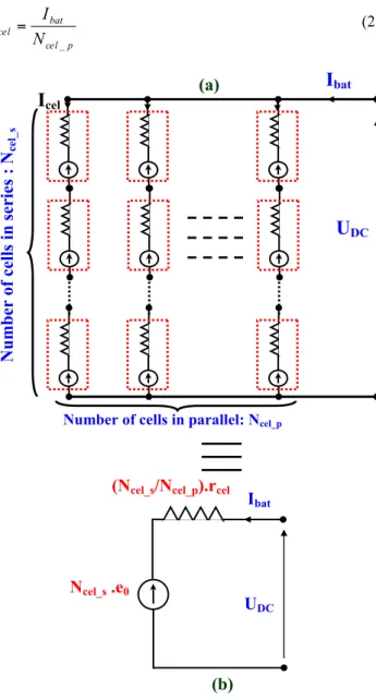
The battery equivalent circuit is deduced from the gathering of elementary cells, as illustrated in 00.

The cell current, used to calculate the SOC depends on the type of association, and is expressed by:

p cel bat cel N I I _ = (23)  

U

DC

N

cel_s

.e

0

(N

cel_s

/N

cel_p

).r

cel

I

bat

U

DC

I

bat

I

cel

Number of cells in parallel: Ncel_p

Number o

f cells

in series

:

N

cel _s

(a)

(b)

Fig. 8. Layout of elementary cells.

0.1 0.2 0.3 0.4 0.5 0.6 0.7 0.8 0.9 1 0 0.5 1 1.5 2 2.5 SOC

r_cel (mΩ)= - 23.12.SOC4 _{+ 53.02.SOC}3 _{- 37.6.SOC}2 _{+ 6.3.SOC + 2.1733}

e₀=-7.6.SOC5+26.4.SOC4 - 33.7.SOC3 + 18.6.SOC2 - 3.5.SOC +1.85

Fig. 9. Evolution of rcel and e0 versus the state of charge. Wind

model

Full analytic model of wind turbine Battery bank model Load model IDC Ibat Iload v UDC UDC Wind model

Full analytic model of wind turbine Battery bank model Load model IDC Ibat Iload v UDC UDC UDC UDC

Fig.10. Synoptic of “full analytic model” blocs’ causality.

A cell is characterized by its internal resistance, r_cel, its load voltage e0, and the voltage at its terminals Vcel

The parameters e0 and rcel vary depending on the SOC of the cell. 0 shows the evolution of these parameters versus the SOC.

The interpolations of measurement points provided by the manufacturer have allowed us to establish the following equations: ⎪⎩ ⎪ ⎨ ⎧ + − + − + − = + + − + − = Ω 8 . 1 . 5 . 3 . 6 . 18 . 7 . 33 . 4 . 26 . 64 . 7 ) ( 18 . 2 . 3 . 6 . 6 . 37 . 53 . 12 . 23 ) ( 2 3 4 5 0 2 3 4 SOC SOC SOC SOC SOC V e SOC SOC SOC SOC m rcel (24)

The expression of the DC bus voltage is then: bat cel p cel s cel s cel DC _N r SOC I N SOC e N U . ( ) ( ) _ _ 0 _ + = (25)

Where:

I

_bat

₌

I

_DC

-

I

_load and Iload is the load current.

Note that the state of charge and consequently the bus voltage UDC are calculated given the load (Iload) and generated (IDC) currents. These currents are time integrated to derive the SOC (22). Consequently, even with the “full analytic model”, no causality problem with subsequent algebraic loops are encountered which reduces the computation time and ensures the numerical stability 0.

4. Battery Bank Sizing Methodologies

The sizing of the battery bank depends on the chosen model: in the first case, with the “mixed reduced model”, in which the battery voltage (i.e. the SOC) is assumed to be constant, the number of battery cells can be synthesized only

from a unique system simulation over the environmental profile (wind data). Contrarily, with the second “full analytic model” which allows coupling bus voltage variations (due to SOC fluctuations), an iterative battery sizing process is necessary.

4.1. Sizing Process Without Soc Variations Coupling (from mixed reduced model)

To size the battery bank using the mixed reduced model, the design methodology is described below. The sizing algorithm uses the battery power given by the following equation:

load WT

BT

P

Losses

P

P

=

−

_∑

−

(26)

The number of battery elements connected in series Ncel_s is not integrated in the sizing problem given that a «nearly constant» bus voltage is assumed from the passive wind turbine structure. However the number of battery strings Ncel_p connected in parallel to yield a desired system storage capacity constitutes the design variable that has to be sized.

The total energy stored by this battery element is given by the following equation:

cel

BT

C

V

E

0

=

₃

.

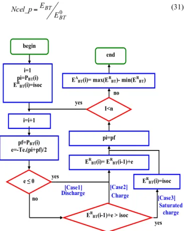
(27)

The algorithm of 0 used to optimally size the battery bank, uses the upper saturated integration method instead of the simple integration method which generally leads to a battery bank over-sizing during wide charge period (huge winds with reduced load) [16-18]. The idea of a saturated integration of the battery power is linked to the fact that charge powers are no more integrated if the battery SOC is maximal. In such a case, we consider that charge power is wasted in order to avoid over-sizing the battery bank. The storage useful energy EBT is given below:

)

(

min

)

(

max

e

t

e

t

E

_BT

=

−

(28) Where,

₍

₎

₍

₎

_[

₀

_,

₂₀₀

_]

0

days

t

d

P

t

e

t BT

∈

=

_∫

τ

τ

Battery charging and discharging current limitations implicate two power based constraints related to energy storage capacity EBT, maximum charging power

P

_BTC and

maximum discharging power

_P

_BTD have to satisfy:

⎪⎩

⎪

⎨

⎧

≤

≤

D BT D BT C BT C BT

E

P

E

P

µ

µ

₍₂₉₎

Where µD is the minimum duration of battery

discharging at

_P

_BTD and µC is the minimum duration of battery charging at P_BTC . Generally, µD is set to a value between 1/5 h and 1 h, while µC is set to a value between 1 h and 2 h. In the case of this study µD and µC are both set to 1 h.

The battery sizing process begins from the integration of the battery power profile (PBT) by initializing the battery relative energy to isoc (initial state of charge). At each step of calculation, the exchanged energy e is computed. Three circumstances are possible:

Ø Circumstance 1: e ≤ 0 (e is discharged from the battery). The exchanged energy e is considered whatever the battery state of charge (soc) value. The new soc is lower than the previous.

Ø Circumstance 2: e > 0 (e is charged in the battery) and soc+e ≤ isoc (battery can still store e). The exchanged energy e is considered to charge the battery. The new state of charge is higher than the previous.

Ø Circumstance 3: e > 0 (e is charged in the battery) and soc+e > isoc (battery is full and can not store e). The exchanged energy e is not considered. The new soc is equal to the previous one.

By considering the discharge rate _kDR _{(set to 80 % in} this case); the battery energy storage capacity EBT is calculated by: DR A BT BT E _k E = (30)  

Where  

_E

_BTA is   defined   in   the   synoptic   of   0   and   corresponds   with   the   maximum   difference   of   battery   energy  over  the  mission  cycle.  

Ncel_p  is  then  given  by  this  equation:  

0 BT BT E E Ncel_p = (31) no ER BT(i-1)+e > isoc yes yes yes no begin i=1 pi=PBT(i) ER BT(i)=isoc i=i+1 pf=PBT(i) e=-Te.(pi+pf)/2 e ≤ 0 ER BT(i)= ERBT(i-1)+e pi=pf I<n EA

BT(i)= max(ERBT)- min(ERBT) end ER BT(i)=isoc [Case1] [Case2] [Case3] Discharge _Charge Saturated charge

Fig. 11. Battery active energy calculation with upper

4.2. Sizing Process with SOC Variations Coupling (from full analytic model)

The global sizing of the storage system by taking account coupling with bus voltage variations (due to SOC variations) is made by using the “full analytic model”. It is performed by iterating the number of parallel battery cells Ncel_p and by simulating the whole system over the wind profile for each of these selected numbers of branches. The search for this number Ncel_p is constrained by boundaries of the battery soc (20% ≤ SOC ≤95%) and of the charging and discharging current maxima. Ncel_p can be obtained using dichotomous search in order to fulfil the target constraints with sufficient accuracy.

Note that a simple management strategy is implemented to disconnect the wind turbine whilst SOC ≥ 95%. This strategy consists to apply an hysteretic control (0) that stops battery charge when the SOC reaches 95% (the recharge is allowed only below 90 %).

5. Results and Discussion

In this section, obtained results for storage system sizing are discussed by comparing both models with the same wind speed profile and for the same power demand during 200 days. This presentation will be completed by a comparative analysis to assess the efficiency of each model in such design process. This comparative analysis phase is completed by the comparison between computational times tCPU required by each model to simulate the behaviour of the passive wind turbine with load and storage association. Simulations are performed with a standard computer (Core Duo 1.7 GHz). 5.1. Results Obtained by the “Mixed Reduced Model”

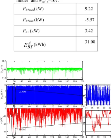
0 presents the evolution of battery power and energy in the case of the “mixed reduced model”. For the battery size, the agreement was obtained by using 107 battery elements in parallel (Ncel_p=107). Further related results are given in 0. 5.2. Results Obtained by “Full Analytic Model”

In the case of the “full analytic model”, the evolution of DC bus voltage battery power and energy are shown in. 0. The number of battery elements in parallel obtained through the battery sizing iterative process is 109 elements (Ncel_p=109). Further related results are given in 0.

SOC IDC=0

IDC

0,9 0,95

Fig. 12. Hysteresis control for charge limit (SOCmax=95%).

0 20 40 60 80 100 120 140 160 180 200 -5 0 5 10 PB T ( kW) 0 20 40 60 80 100 120 140 160 180 200 -40 -30 -20 -10 0 time(days) e (k W) 14 16 18 20 22 -6 -4 -2 0 2 4 6 8 9.5 14 16 18 20 22 -30 -25 -20 -15 -10 -5 0 ZOOM ZOOM

Fig. 13. Evolution of battery power and energy obtained with

the “mixed reduced model”.

Table.3. Sizing variables obtained with the “mixed reduced

                             

model” and Ncel_p=107.

 

PBTmax(kW) 9.22 PBTmin (kW) -5.57 PAV (kW) 3.42 A BT

E

(kWh) 31.08 0 20 40 60 80 100 120 140 160 180 200 47.5 48 48.5 UD C ( V ) 0 20 40 60 80 100 120 140 160 180 200 -5 0 5 10 PBT ( kW) 0 20 40 60 80 100 120 140 160 180 200 -30 -20 -10 0 time(days) e (k W) 14 16 18 20 22 -5 -3 0 2 6 9 14 16 18 20 22 -30 -20 -10 ZOOM ZOOM

Fig. 14. Evolution of UDC, battery power and energy obtained with the “full analytic model”.

Table.4. Sizing variables obtained with the “full analytic

model” and Ncel_p=109.

PBTmax(kW) 9.22 PBTmin (kW) -5.57 PBTAV (kW) 3.14 A BT

E

(kWh) 31.63

Table.5. Comparison between results obtained by both models.

     

Mixed reduced model Full analytic model ratio Ncel_p 107 109 1.02 PBTAV(kW) 3.42 3.14 0.92 PBTmin (kW) -5.57 -5.57 0 PBTmax (kW) 9.22 9.22 0 tCPU (s) 16.4 39.5 2.4

5.3. Analysis and Comparison

0 summarizes the results obtained by both models and gives the ratio between each sizing variable. On the one hand, with the “full analytic model”, the noticed decreasing of the average battery power is expected, since this model takes into account DC bus voltage variation which results in power degradation.

On the other hand, computational time necessary for the “mixed reduced model” is reduced by a ratio of 2.4 compared with that necessary for the “full analytic model”. This is mainly due to the iterative process used in each calculation step, to solve the sixth order equation and select the positive root adequate for determining the rotational speed. This reduction will have major repercussion in the case of design by optimization when computational time is a crucial factor. Oppositely, the sizing process accuracy is increased by taking account of SOC variations (i.e. UDC level) for wind power extraction quality.

In addition, we conclude that both models used to design a passive wind turbine with storage subjected to the same wind speed profile and the same consumption have given quite similar results for battery sizing variables with a reduction of computational time in case of use of mixed reduced model. Therefore, the above results indicate that mixed reduced model can be feasibly utilized in a design by optimization context since it offers a reduction of computational time with an acceptable accuracy regarding the full analytic model.

6. Conclusion

In   this   study,   two   stand-alone wind turbine system models   for   sizing a battery bank have been developed and analyzed. The first model requires only information on the power exchanged from the battery with the rest of the system by considering the battery voltage as constant regardless of its state of charge. Therefore, it is possible to size the battery with a direct synthesis process without iteration. In contrast, the coupling between changes in DC voltage and the battery state of charge is considered in the second model. The passive wind turbine is subjected to the same wind speed profile and the same consumption. Both models led to quite similar results for sizing the battery bank with a reduction of computational time given by the mixed reduced model. In the context of the optimization process of such systems,

reduction of the computation time is a primordial factor for a designer and the choice of mixed reduced model seems more pertinent in such problems.

 

Acknowledgements

This work was supported by the Tunisian Ministry of High Education, Research and Technology; CMCU- 12G1103 and INPT SMI projects.

References

[1] M. Uzunoglu, OC. Onar, MS. Alam, “Modelling, control and simulation of a PV/FC/UC based hybrid power generation system for stand-alone applications”, Renewable Energy; 34(3):509–20, 2009.

[2] J. Lagorse, D. Paire, A. Miraoui, “Sizing optimization of a stand-alone street lighting system powered by a hybrid system using fuel cell, PV and battery”, Renewable Energy;34(3):683–91, 2009.

[3] El-T. Shatter, M. Eskander, M. El-Hagry. “Energy flow and management of a hybrid wind/PV/fuel cell

generation system”, Energy Conversion and

Management, 47(9–10):1264–80, 2006.

[4] JA. Baroudi, V. Dinavahi, AM.Knight, “A review of power converter topologies for wind generators”, Renewable Energy;32:2369–85, 2007.

[5] B. Sareni, A. Abdelli, X. Roboam, D.H. Tran, “Model simplification and optimization of a passive wind turbine generator”, ISSN: 0960-1481, Elsevier Renewable Energy 3, pp. 2640-2650, 2009.

[6] J. Belhadj, X. Roboam, “Investigation of different methods to control a small Variable Speed Wind Turbine with PMSM Drives”, ASME Journal of Energy Resources Technology, September 2007 -- Volume 129, Issue 3, pp. 200-213, 2007.

[7] A. Mirecki, X. Roboam, F. Richardeau, “Architecture cost and energy efficiency of small wind turbines: which system tradeoff?”, IEEE Transactions on Industrial Electronics, February;54(1):660–70, 2007.

[8] D.H. Tran, B. Sareni, X. Roboam, C. Espanet, “Integrated Optimal Design of a Passive Wind Turbine System: An experimental validation”, IEEE Transactions on Sustainable Energy, Vol. 1, n°1, pp. 48-56, 2010. [9] Y. Fefermann, S. A. Randi, S. Astier, X. Roboam,

‘’Synthesis models of PM Brushless Motors for the design of complex and heterogeneous system’’, EPE’01, Graz, Austria, September 2001.

[10] X. Roboam, A. Abdelli, B. Sareni, "Optimization of a passive small wind turbine based on mixed Weibull-turbulence statistics of wind", Electrimacs 2008, Québec, Canada, 2008.

[11] X. Roboam, A. Abdelli, B. Sareni, "Optimization of a passive small wind turbine based on mixed

Weibull-turbulence statistics of wind", Electrimacs 2008, Québec, Canada, 2008.

[12] Y.-K. Chin, J. Soulard “Modelling of iron losses in permanent magnet synchronous motors with field weakening capability for electric vehicles”, International Journal of Automotive Technology, Vol. 4, No. 2, pp. 87-94 ,2003.

[13] E. Hoang, B. Multon, M. Gabsi, “Enhanced accuracy method for magnetic loss measurement in switched reluctance motor”, ICEM’94; 2:437–42, 1994.

[14] http://www1.futureelectronics.com/doc/IXYS

[15] S. Piller, M. Perrin, A. Jossen, “Methods for state-of-charge determination and their applications”, Journal of Power Sources, Elsevier, pp. 113-120, 2001.

[16] http://www.houseofbatteries.com/pdf/NP38-12

[17] R. Belfkira, C. Nichita, P. Reghem, G. Barakat, “Modeling and optimal sizing of hybrid energy system”, International Power Electronics and Motion Control Conference (EPE-PEMC), September 1-3, Poznan, Poland, 2008.

[18] C.R. Akli, X. Roboam, B. Sareni, A. Jeunesse, “Energy management and sizing of a hybrid locomotive”, 12th International Conference on Power Electronics and Applications (EPE'2007), Aalborg, Denmark, 2007 [19] R. Belfkira, G. Barakat, C. Nichita, “Sizing

optimization of a stand-alone hybrid power supply unit: wind/PV system with battery storage”, International Review of Electrical Engineering (IREE), Vol. 3, No. 5, October 2008.