Simulation of temperate freezing lakes by one-dimensional lake models: performance assessment for interactive coupling with regional climate models

Texte intégral

(1)Boreal Environment Research 15: 143–164 © 2010 ISSN 1239-6095 (print) ISSN 1797-2469 (online) Helsinki 30 April 2010. Simulation of temperate freezing lakes by one-dimensional lake models: performance assessment for interactive coupling with regional climate models Andrey Martynov*, Laxmi Sushama and René Laprise Centre ESCER, Université du Québec à Montréal, CP 8888, succursale Centre-Ville, Montréal (Québec) Canada, H3C 3P8 (corresponding author’s e-mail: andrey.martynov@uqam.ca) Received 17 Feb. 2009, accepted 7 Oct. 2009 (Editor in charge of this article: Kai Myrberg) Martynov, A., Sushama, L. & Laprise, R. 2010: Simulation of temperate freezing lakes by one-dimensional lake models: performance assessment for interactive coupling with regional climate models. Boreal Env. Res. 15: 143–164.. A systematic assessment of the ability of two selected 1-D lake models (the model of S.W. Hostetler and the Freshwater Lake model) to simulate lake surface temperature and fluxes for different lake conditions, corresponding to typical temperate freezing lakes of North America, through a set of offline tests, is presented. Results suggest that both models perform well in shallow lakes, while important differences between modelled and observed water temperatures and ice-cover duration can be noticed in deeper lakes. These differences could be partially attributed to the biases in the driving data and most importantly to the lack of representation of complex processes in the models, such as horizontal transfer of water and heat, ice drift, etc. Sensitivity of the models to lake depth, water transparency, explicit snow and snow/ice albedo is presented and possible ways of improving the performance of the 1-D lake models are proposed.. Introduction Lakes are an important component of the climatic system and they can influence the local climate in many ways. Air masses, when passing over lakes, are modified due to moisture, thermal and frictional differences between the lake surfaces and upwind land areas (Kristovich and Braham 1998). The great thermal inertia of lakes usually reduces the diurnal and annual temperature ranges over and in the vicinity of lakes (Long et al. 2007). The well-known example of the lake influence is the lake-effect snow that occurs on the downwind coastal area of many large and mid-sized temperate lakes in winter (Liu and Moore 2004, Laird et al. 2009). Smaller lakes. influence local climate to a lesser extent (Kodama et al. 1983) but in regions where lakes are abundant, such as the Canadian Shield or Scandinavia, the cumulative effect of lakes on the local climate can be important (Rouse et al. 2008). Given the above, it is essential to represent lakes adequately in climate models to produce realistic near-surface climate. Current Regional Climate Models (RCMs) are capable of resolving large to medium lakes. These resolved and unresolved lakes (i.e. sub-grid lakes), can be represented using lake models, interactively coupled with RCMs. Different lake models have been developed and considered for coupling with RCMs. For example, a simple mixed-layer model, devel-.

(2) Martynov et al. • Boreal Env. Res. Vol. 15. 144. oped by Goyette et al. (2000) is implemented in the Canadian Regional Climate Model (Laprise 2008) for the Great Lakes; this model involves calculation of heat-flux residuals prior to using the model and becomes computationally expensive. Such an approach is also questionable when used for climate-change projections. In vertically-resolved 1-D lake models, lakes are treated as horizontally homogeneous vertical “wells”, with no explicit horizontal interactions. Sophisticated three-dimensional lake/ocean models, such as Princeton Ocean Model (POM), Estuary Lake and Coastal Ocean Model (ELCOM), Nucleus for European Modelling of the Ocean (NEMO), are capable of simulating the water circulation in lakes, and the interactive coupling of climate models with 1-D models (Hostetler 1993) and complex 3-D models (Song et al. 2004) had been proposed and tested in the past. Swayne et al. (2005), based on their study of suitability of lakes in RCMs, suggested using 1-D, 2D and 3-D lake models for small, medium and large lakes, respectively. Recently, a 3-D lake model study of the Great Slave Lake was carried out in view of using this model interactively in RCMs (Leon et al. 2007). Coupling an RCM with complex 3-D lake models would, however, add much to the complexity of the model and require considerable computational power. The horizontal resolution of 3-D lake models is 2.0–2.5 km, which largely exceeds the horizontal resolution of modern RCMs. Thus, 1-D lake models are a convenient choice for interactive coupling with RCMs. Regional climate models, depending on the study domain, need to deal with a variety of lakes, located in different geomorphologic zones, and in different climatic conditions. Existing lake models have limitations, when it comes to the processes and therefore lake models applicable to shallow lakes may not be good for deep lakes. In addition, the exact values of important lake parameters, such as lake depth and water transparency, are often not known, especially for medium-sized and small lakes, and averaged or arbitrary values are often used instead. It is important therefore to assess the limitations of various lake models, used for coupling with RCMs and to study the sensitivity of these models to key lake parameters, in order to esti-. mate the errors that might be introduced due to lake parameter uncertainties. In this article, the performance of two 1-D lake models is studied and their sensitivity to lake depth, water transparency, ice/snow albedo, and to the presence or absence of explicit snow cover are studied.. Lake models Two lake models, widely used for coupling with climate models and able to simulate freezing lakes, are considered in this study: the FLake model (Mironov 2008, Mironov et al. 2010), and the model developed by Hostetler et al. (1993). These models are described below. The lake model of Hostetler solves the vertical thermal diffusion equation with a wind-driven eddy turbulence parameterized as enhanced thermal diffusion based on Henderson-Sellers (1985) as follows: , (1) where θ(z,t) is the water potential temperature at the depth z in the moment t, f the heat sources (absorption of the penetrating solar radiation), c the water heat capacity, and km the molecular heat diffusivity in water (1.38889 ¥ 10–7 m2 s–1). K(z,t) the effective eddy diffusion is given by in neutral conditions and. (2) in stably stratified conditions,. where w* = 1.2 ¥ 10–3U (m s–1) is the friction velocity, U is the wind speed, kek is the latitude parameter, P0 is the Prandtl number in neutral conditions (1.0), k is the von Karman constant (0.4), and Ri is the Richardson number. The model assumes zero heat flux at the bottom of the lake. It is important to mention that in winter conditions, when the ice insulates the lake from the atmosphere, the wind-driven mixing is absent (U = 0, K(z,t) = 0) and only molecular diffusion km remains in Eq. 1. The model includes gravitationally-driven convection, mixing the.

(3) Boreal Env. Res. Vol. 15 • Simulation of temperate freezing lakes by one-dimensional lake models. water layers once density inversion is detected. The mixed-layer depth, a diagnostic parameter in the Hostetler model, is determined by the iterative mixing between the water surface and deep water layers, until the mixed profile becomes stable. All the incoming UV radiation and 40% of non-reflected SW radiation is absorbed at the water surface, the remaining SW radiation penetrates the water column and its absorption follows the Beer-Lambert law. The ice and snow model is based on the modified Patterson and Hamblin (1988) model. The temperature within the ice/snow layers is obtained as a solution of the heat diffusion equation with the molecular ice/snow diffusivity, taking into account the partial penetration of solar radiation into snow and ice. Ice grows when the water temperature is below freezing point and the surface energy balance is negative. The model takes into account snow and ice melting and ablation. The snow/ice conversion processes are not taken into account. In the absence of snow, or if the snow depth is below some minimum value (five centimetres usually), the shortwave albedo is calculated, using an approximate dependence on the air temperature. Albedo values during the winter are usually between 0.2 and 0.3. In the presence of a thicker snow layer, fresh snow albedo is used (0.7). The ice model allows fractional ice coverage, where a fraction of surface remains open until the ice thickness exceeds some pre-defined value (usually 10 cm). Separate calculations of the water temperature profiles are performed for open and ice-covered fractions at every time step, followed by an areaweighted averaging to determine the effective water temperature profile. The latent and sensible heat fluxes for off-line simulations are calculated using a standard surface drag coefficient formulation based on surface-layer similarity theory. The drag coefficient calculations follow the Biosphere–Atmosphere Transfer Scheme (BATS) formulation (Dickinson et al. 1993). The FLake model is based on the concept of self-similarity of the thermal structure of the water column. This concept originates from observations of oceanic mixed layer dynamics (Kitaigorodskii and Miropolsky 1970). A twolayered water temperature profile is assumed, with the mixed layer at the surface, and the ther-. 145. mocline extending from the lake bottom to the base of the mixed layer. The shape of thermocline is parametrized using a fourth-order polynomial function of the depth FT, depending on a shape coefficient CT. Equations 3–5 describe the thermal structure of the water column in the FLake model: (3) (4). (5) where z is the depth, θ(z,t) is the water potential temperature, h is the mixed-layer depth, D is the lake depth, z is the dimensionless depth in the thermocline layer. The value of the shape coefficient CT lies between 0.5 and 0.8 in the model for reasons of numerical stability. This means that the thermocline can neither be very concave nor very convex (Mironov 2008: fig. 5). The same parametric concept is applied to the ice and snow layers (with linear shape functions) and to the bottom sediment layer. Instead of the active sediment layer, the zero bottom heat flux condition can be used. The UV radiation is absorbed at the water surface, and the non-reflected SW radiation penetrates the water column and is absorbed in accordance with the Beer-Lambert law. A system of prognostic ordinary differential equations is solved for the thermocline shape coefficient, the mixed-layer depth, bottom and surface water temperatures, shape parameter and temperature of the active sediment layer, as well as ice and snow temperatures. The mixed-layer depth equation includes convective entrainment, wind-driven mixing and volumetric solar radiation absorption. The two-layer water temperature parameterization limits the applicability of the FLake model to deep lakes, because it does not allow for the hypolimnion layer between the thermocline and the lake bottom. Consequently, in such cases, a “virtual bottom”, usually at 40 to 60 meters, is used in simulations, instead of the real lake depth. The parametric structure of.

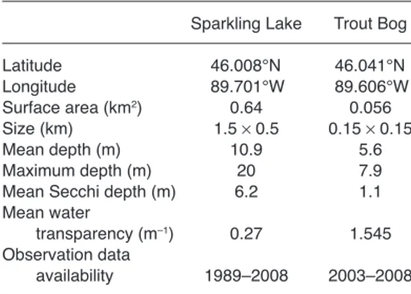
(4) Martynov et al. • Boreal Env. Res. Vol. 15. 146. the FLake model does not allow for partial ice coverage, as in Hostetler’s model. The snow module is present in the FLake model, however its use is not recommended by model developers. Instead, a correction of the ice albedo, taking into account the influence of the snow cover, is applied. Its value is usually between 0.2 and 0.3. The surface heat fluxes are calculated, based on the Charnock formula with the Charnock parameter obtained from the wind fetch, using an empirical equation. The scalar roughness lengths are based on the power-law formulations in terms of the roughness Reynolds number (Zilitinkevich et al. 2001).. Off-line lake model simulations The goal of off-line model experiments is to assess lake model performance in conditions, corresponding to different lake types, using observed or reanalysed datasets as model inputs. It should be noted that in most cases surface heat flux observations are not long and complete enough or are not of suitable quality to be used as direct input to lake models. Therefore, it is necessary to calculate these fluxes on the basis of meteorological observations that are generally available. The two lake models were applied to two small and shallow temperate lakes and to the Great Lakes. The obtained results are compared with observation data and climatological means, where available.. Table 1. Basic characteristics of Sparkling Lake and Trout Bog, Wisc., USA (NTL LTER project). Sparkling Lake Trout Bog Latitude Longitude Surface area (km2) Size (km) Mean depth (m) Maximum depth (m) Mean Secchi depth (m) Mean water transparency (m–1) Observation data availability. 46.008°N 89.701°W 0.64 1.5 ¥ 0.5 10.9 20 6.2. 46.041°N 89.606°W 0.056 0.15 ¥ 0.15 5.6 7.9 1.1. 0.27. 1.545. 1989–2008. 2003–2008. Small lakes The two small lakes, Sparkling Lake and Trout Bog (Table 1), simulated using the lake models, are located in Vilas County, Wisconsin, USA, and are representative in size of sub-grid lakes in an RCM. They are located in a forested, moderately developed landscape, typical of the North American temperate zone. Both lakes are freezing, freshwater and dimictic, with complete water overturning twice a year, in spring and in autumn. These lakes were chosen due to the availability of year-round, high-quality meteorological and hydrological data for long periods through the North Temperate Lakes Long Term Ecological Research program (NTL LTER, www.lternet.edu/sites/ntl). For simulations, the following raft data (one-hour averaged values) were used as model input (NTL LTER datasets at http://lter.limnology.wisc.edu): air temperature, wind speed, relative humidity (all at two-meter height) as well as hourly precipitation rate. The downward shortwave and longwave radiation fluxes were not available for the lakes. Instead, measurements at the nearby Minocqua-Woodruff Lakeland Airport meteorological station (12 km south of the lakes) were used. Mean Secchi depth values were used for estimation of water transparency (Idso and Gilbert 1974). Another set of observation data was used for validation of model results: buoy-measured surface water temperature, water temperature profiles, and latent and sensitive heat fluxes (available only for the Sparkling Lake). The ice thickness was measured two or three times per season, and the first freezing and complete ice meltdown dates are also available in this dataset. Based on the availability and quality of the observation data, the year 2005 was chosen for simulations. The simulations were carried out in a perpetual year regime by repeating one-yearlong simulations several times until the equilibrium solution was obtained. Both models were run with a timestep of one hour. The vertical resolution in the Hostetler model was 1 meter. In order to estimate the performance of both models in similar configurations, the snow modules in both models, the partial ice cover mechanism in the Hostetler model, and the active sediment module in FLake were turned off..

(5) Mixing depth (m). Fig. 1. Observed and model-simulated annual thermal cycles for the Sparkling Lake: (a) water surface temperature, (b) ice thickness, (c) mixed layer depth (no observations).. 147. Ice thickness (m). Water surface temperature (°C). Boreal Env. Res. Vol. 15 • Simulation of temperate freezing lakes by one-dimensional lake models. The observed surface temperature of Sparkling Lake is very closely reproduced by both models (Fig. 1a and Table 2). It is important to note the rapid rise of the water surface temperature just after the disappearance of ice in spring, according to the Hostetler model. The ice cover thickness and duration are well reproduced by both models (Fig. 1b). The mixed-layer depth in summer is generally close in both models (see Fig. 1c). The rapid variations of the mixed-layer depth in Hostetler model simulations reflect the diurnal surface-water heating variability with stratified daytime profiles and convectively mixed profiles at night. Both models reproduce the dimictic mixing regime of the lake, with two seasonal overturnings, although the spring overturning period is very short in the Hostetler. model simulation. The simulated ice cover thickness is close to observations for both models and the ice cover duration is also reasonably well reproduced. Both models reproduce well the annual evolution of the thermal structure (Fig. 2): the autumn and spring overturnings, the stratification in spring and early summer, and the deepening of the mixed layer during late summer and autumn cooling. For FLake, the ice formation (“ice freeze-up”) occurs earlier and the ice disappearance (“ice break-up”) later, as compared with the Hostetler model. In winter, however, strong differences can be seen between observed water temperature profiles and those simulated by the models. In winter, in the presence of ice cover, there is no wind-driven turbulence and only molecular ther-. Table 2. Statistics of simulations of the Sparkling Lake by two 1-D lake models. Source of data Observations Hostetler model. FLake model. Annual mean water surface temperature (°C) 10.1 Root mean square deviation from observations (°C) Pearson correlation with observations Open water/ice covered sensible heat flux (W m–2) –25.6/–37.12 Root mean square deviation from observations (W m–2) Pearson correlation with observations Open water/ice covered latent heat flux (W m–2) –62.9/–25.9 Root mean square deviation from observations (W m–2) Pearson correlation with observations . 10.2 3.2 0.98 –35.6/–19.8 24.3/35.6 0.59/0.29 –62.5/–12.7 28.1/19.6 0.82/0.56. 10.1 1.8 0.98 –39.4/–15.9 24.3/30.8 0.66/0.43 –70.8/–16.6 18.6/28.9 0.93/0.32.

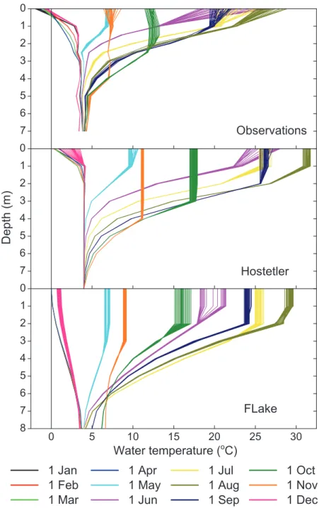
(6) 148. Martynov et al. • Boreal Env. Res. Vol. 15. Fig. 2. Observed and model-simulated annual and diurnal evolutions of water temperature for Sparkling Lake. Hourly water temperature profiles are shown for the 1st day every month of the year.. mal conductivity is considered in the Hostetler model. This leads to the formation of neutral, vertically homogenous profiles of temperature, close to the maximum density temperature, of 4 °C, except for the uppermost layer, where the temperature rapidly decreases to (almost) 0 °C at the lower surface of the ice cover. In the two-layer FLake model, due to the absence of the wind-driven turbulence under ice, the whole water column represents a thermocline. The shape function (see Eq. 5) can vary only. within certain limits and, thus, generates smooth, stratified water temperature profiles under ice. The difference between models can be also seen in the diurnal cycle simulation (Fig. 3b). The diurnal variability is almost absent, when the lake is ice-covered; it is strongest in late spring and summer, i.e. during the period of strong stratification, when the stable water column prevents rapid mixing of the uppermost water layer with deeper water layers. The Hostetler model reproduces this effect (see Fig. 2), but in FLake,.

(7) Boreal Env. Res. Vol. 15 • Simulation of temperate freezing lakes by one-dimensional lake models. 149. Fig. 3. (a) The annual water surface temperature cycles, and (b) the diurnal variations of the water surface temperature for Sparkling Lake, for the 1st day of every month (green bars).. where the constant-temperature mixed layer is implied, complete mixing within the mixed layer is forced, which reduces the diurnal temperature variations (see Fig. 3). The diurnal variation is decreases strongly in autumn, during the cooling phase, when the surface cooling causes strong convective mixing in the upper part of the water column. The high variability produced by the Hostetler model on the 1 December 2005 is caused by the rapid surface cooling that occurred this day after crossing the maximum density temperature of 4 °C (see Fig. 3a). Over open water, both sensible and latent heat fluxes are well reproduced by both models (Fig. 4 and Table 2). During winter, in the presence of ice cover, both models tend to underestimate substantially the sensible and latent heat fluxes in comparison with observed data. The correlations between simulated heat fluxes and. observations are much lower in the presence of ice cover, than for the open water cases. It is important to note, however, that observation of heat fluxes in winter is often tedious and the possibility of observational errors can not be completely excluded. The second simulated lake, Trout Bog, is a quiet, small (150 m in diameter) and shallow (7-m deep) forest pond. As in the case of Sparkling Lake, the annual thermal cycle of Trout Bog is well reproduced by both models. It is important to note that, when ice-covered, the measured water temperature is almost constant, with only a thin gradient zone close to the surface (Fig. 5). These temperature profiles, reflecting the small thermal conductivity in the lake water, are similar to those produced by the Hostetler model under the assumption of molecular thermal conductivity alone in the presence of ice cover..

(8) 150. Martynov et al. • Boreal Env. Res. Vol. 15. Fig. 4. Comparison of observed and simulated sensible and latent heat fluxes in Sparkling Lake: (a) sensible heat, simulated by the Hostetler model, (b) latent heat, simulated by the Hostetler model, (c) sensible heat, simulated by the FLake model, (d) latent heat, simulated by the FLake model.. Great Lakes In the second stage of the offline tests, the lake models were applied to the Laurentian Great Lakes, which are deep and large as compared. with the lakes described in the previous section. Lake Superior, the largest of the Great Lakes, is represented by 52 grid cells, while Lake Michigan, Lake Huron, Lake Erie and Lake Ontario are represented by 37, 33, 17 and 10.

(9) Boreal Env. Res. Vol. 15 • Simulation of temperate freezing lakes by one-dimensional lake models. 151. Fig. 5. Observed and model-simulated annual and diurnal evolutions of water temperature for Trout Bog. Hourly water temperature profiles are shown for the 1st day of every month of the year.. grid cells, respectively (Fig. 6). In the absence of the observed meteorological data over the Great Lakes, with required horizontal resolution and continuity, or of publicly available reconstructions of meteorological conditions over the Great Lakes as used in Beletsky and Schwab (2001), interpolated ERA40 reanalysis data (Uppala et al. 2005) were used as inputs in this simulation: air temperature and humidity, wind components. (all at two-meter height) and downward solar and infrared radiation fluxes. The archival interval of the ERA40 data is six hours; the atmospheric data were linearly interpolated to produce the hourly input datasets, while the shortwave and infrared radiation fluxes were kept constant during each six-hour period. A 30-year (1971–2000) simulation of the Great Lakes water and ice evolution is performed, preceded by a 10-year-long spin-up..

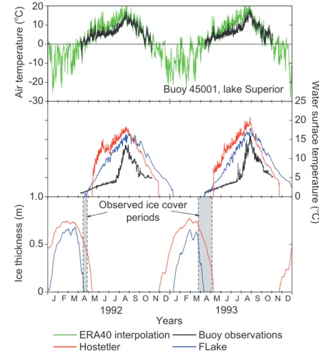
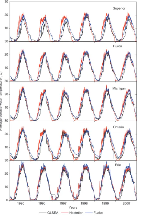
(10) 152. Martynov et al. • Boreal Env. Res. Vol. 15. Fig. 6. Great Lakes on a polar stereographic grid with a horizontal resolution of 45 km (true at 60°N), similar to the resolution of most RCMs and positions of selected NDBC buoys in polar stereographic coordinates.. Following the recommendations for the FLake model (http://www.flake.igb-berlin.de/papers/ flake_synopsis.pdf), the simulation depth for this model was limited to 60 meters. As in the case of small lakes, the snow modules were turned off in both models and a vertical resolution of 1 m was used for the Hostetler model. For validation of the results, following datasets were used: the observation data (air temperature and water surface temperature) from several NDBC buoys (Fig. 6), the GLSEA average surface water temperatures (Schwab et al. 1999), and the GLERL Great Lakes Ice Atlas (Assel 2003). The air temperatures at the surface, measured by buoys, is different from the interpolated ERA40 values used to drive the lake model, especially during the spring and summer periods (Fig. 7). For Lake Superior, the differences between the measured and simulated water surface temperatures are significant (Fig. 7). For Lake Michigan (Fig. 8), differences are not so pronounced, and they are minimal for the shallow Lake Erie (Fig. 9). Both models predict longer ice cover periods in winter, than what is observed. The scarcity of direct observation data over the Great Lakes for the simulated period can partially be compensated by the Great Lakes Surface Environmental Analysis (GLSEA), the satellite-based averaged surface water data for each of the Great Lakes, produced by the CoastWatch project of GLERL (Schwab et al. 1999) for the 1995–2004 period. In accordance with the buoy data (see Figs. 7–9) discussed above,. the strongest differences between simulated and satellite-based temperatures are for Lake Superior, the deepest and coldest of all the Great Lakes, while for Lake Erie, the shallowest of all the Great Lakes, the simulated temperatures are close to observations (Fig. 10 and Table 3). One of the most important features of these simulations is the marked distinction between the spring warming patterns in the observations and simulations. The simulation with the Hostetler model reproduces the same patterns, which are present in shallow lakes: very rapid cooling in autumn, once the surface temperature drops below 4 °C, and very rapid warming in spring, after complete ice break-up (Fig. 7). This behavior differents from the characteristic pattern captured by the buoy observations in lakes Superior and Michigan (Figs. 7 and 8): prolonged (2–3 months) and slow warming of the surface water from 0 °C to 4 °C reflects the presence of a deep convective mixed layer during this period. This pattern is typical for central parts of large deep freezing lakes (Beletsky and Schwab 2001), when the complex circulation structure with the thermal bar is formed during spring warming (Boyce et al. 1989). The existence of deep mixed layer in winter in the presence of ice cover was confirmed by measurements from Lake Huron (Assel 1986.) The very fast warming, occurring in the Hostetler model simulations, results from the assumption of the water thermal diffusivity in the absence of the wind-driven eddy turbulence,.

(11) Boreal Env. Res. Vol. 15 • Simulation of temperate freezing lakes by one-dimensional lake models. 153. Fig. 7. Model-simulated air temperature, water surface temperature and ice thickness for the Great Lakes in comparison with observations from buoy 45001, central Lake Superior.. shielded by the ice cover. As described above, this leads to quasi-homogenous water thermal profiles at the maximum density temperature (4 °C), with a thin gradient layer below ice. Such conditions can be met in shallow, small and quiet lakes like Trout Bog, but in deep and large freezing lakes, observations suggest presence of mixing under the ice cover. It was proposed by Bates et al. (1995) that the model performance can possibly be improved by increasing the background thermal diffusivity in water. Here, the surface water temperature starts being affected only at very high values of diffusivity (103km–104km) (see Fig. 11). Decreasing water temperature in summer demonstrates stronger vertical heat redistribution in stratified conditions. The open-water period duration increases with diffusivity and, in the shallow Lake Erie, the winter ice cover disappears at 103km. Pos-. sibly, more complex modification of the model than simple increase of the background thermal diffusivity are required for improving the model performance in deep freezing lakes. In the FLake model, the rigid two-layer water column structure, with the thermocline extending between the mixed layer and the lake bottom, assumes certain water mixing under the ice cover, even in the absence of wind-driven turbulence. The structure of this model makes it difficult to introduce modifications to the formulation. To some extent, additional mixing can be introduced in FLake by modifying the prescribed lake depth. Since the FLake simulations are very sensitive to the lake depth (Fig. 12), using actual depth in deep lakes can lead to incorrect results. The simulation for the depth of 180 meters (Fig. 12) can be compared with the data from the NDBC buoy 45002 (181 m) in Lake.

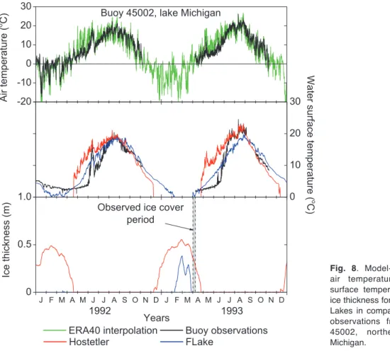
(12) 154. Martynov et al. • Boreal Env. Res. Vol. 15. Fig. 8. Model-simulated air temperature, water surface temperature and ice thickness for the Great Lakes in comparison with observations from buoy 45002, northern Lake Michigan. Table 3. Statistics of simulations of the Great Lakes by two 1-D lake models (surface-averaged) and of Great Lakes Surface Environmental Analysis (GLSEA) data, 1995–2000.. GLSEA Hostetler model. Lake Superior Mean annual water surface temperature (°C) 6.2 Root mean square deviation from GLSEA (°C) Pearson correlation with GLSEA Lake Michigan Mean annual water surface temperature (°C) 9.4 Root mean square deviation from GLSEA (°C) Pearson correlation with GLSEA Lake Huron Mean annual water surface temperature (°C) 8.7 Root mean square deviation from GLSEA (°C) Pearson correlation with GLSEA Lake Erie Mean annual water surface temperature (°C) 11.3 Root mean square deviation from GLSEA (°C) Pearson correlation with GLSEA Lake Ontario Mean annual water surface temperature (°C) 9.8 Root mean square deviation from GLSEA (°C) Pearson correlation with GLSEA . FLake model. 8.1 3.8 0.86. 8.0 2.2 0.95. 10.9 3.0 0.94. 11.0 1.6 0.98. 9.9 2.8 0.94. 9.9 1.5 0.98. 12.5 2.3 0.96. 12.9 2.5 0.97. 11.3 2.7 0.94. 11.5 1.9 0.97.

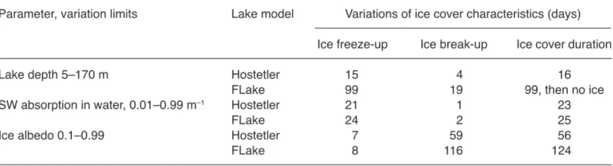
(13) Boreal Env. Res. Vol. 15 • Simulation of temperate freezing lakes by one-dimensional lake models. 155. Fig. 9. Model simulated air temperature, water surface temperature and ice thickness for the Great Lakes in comparison with observations from buoy 45005, western Lake Erie.. Michigan. The resulting temperature profile is, evidently, not realistic. The maximum lake depth of 60 meters, suggested by the FLake model synopsis and used in the presented Great Lakes simulations, appears to be a good compromise. The maximum depth value, however, remains an arbitrary parameter, which can hardly be deduced from physical considerations.. Sensitivity studies Sensitivity studies were carried out for the Sparkling Lake. Same settings as described earlier were used, except for the parameter studied, which is varied within a certain range. The sensitivity of lake models was assessed, based on ice phenology and other lake characteristics (water. Table 4. Variations in ice freeze-up, ice break-up dates and in the total duration of the ice cover, caused by variations of lake depth, water transparency and ice albedo. Parameter, variation limits Lake model Variations of ice cover characteristics (days) Ice freeze-up Ice break-up Ice cover duration Lake depth 5–170 m Hostetler. FLake SW absorption in water, 0.01–0.99 m–1 Hostetler. FLake Ice albedo 0.1–0.99 Hostetler. FLake. 15 99 21 24 7 8. 4 19 1 2 59 116. 16 99, then no ice 23 25 56 124.

(14) 156. Martynov et al. • Boreal Env. Res. Vol. 15. Fig. 10. Average surface water temperatures for the Great Lakes, simulated by the lake models and those from the Great Lakes Surface Environmental Analysis data.. surface temperature, mixed layer depth, surface heat fluxes) (see Table 4). Lake depth Climate models require information about average lake depth for lakes coupled with the models. Due to the lack of lake-depth information, in RCMs that currently have coupled lakes, arbitrary. lake depths are assigned. For example, in the Rossby coupled model, lake depths are assumed to be 10 m, when lake depth data are not available (Samuelsson et al. 2010). Our analyses proved that at very small lake depths, around five meters, mixing is almost complete during the warm period (Fig. 12). In the Hostetler model simulations, the ice freeze-up and ice break-up dates depend on the lake depth only at low lake depths (total variations: 15 days and four days, respectively) and.

(15) Boreal Env. Res. Vol. 15 • Simulation of temperate freezing lakes by one-dimensional lake models. the ice cover duration decreases with depth (Fig. 13). For lake depths exceeding 20 meters, the ice cover duration does not depend anymore on lake depth. The difference in the ice cover duration for lake depths of five and 70 meters is 16 days. In FLake, much larger changes are noticed. While the ice break-up date shifts slowly to earlier dates with the lake depth (total variation is 19 days for lake depths of five and 55 meters), the ice freeze-up date shifts rapidly to later dates (total variation: 99 days), thus the total ice cover duration is reduced with depth and ice disappears completely for lake depth of 56 meters. These differences between the two lake models result from differences in their physical formulations. In the Hostetler model, when the lake depth exceeds the depth of penetration of the wind-driven turbulence and the mixed layer depth, a thermally homogenous bottom water layer, or hypolimnion, is formed. Further increase of the lake depth only leads to thickening of this layer, leaving the surface mixing untouched. In the FLake model the thermocline extends to the bottom and with growing lake depth, the heat content in deep water layers increases, leading to slow cooling of water in autumn and later ice formation. The twolayered structure of the FLake model does not allow for the formation of the hypolimnion layer in deep lakes and thus, the strong dependence of the ice cover duration on the lake depth in FLake simulations is artificial (Fig. 13). Water transparency Water transparency determines the absorption of solar radiation, penetrating into the lake water. In highly transparent waters, solar radiation penetrates deep into the water column, heating up deeper water layers, thus reducing the water temperature stratification and the water column stability. On the contrary, in turbid waters, solar radiation is absorbed in upper water layers, thus heating up the water surface and increasing the temperature stratification. Thus, a deeper mixed layer is formed in summer in transparent waters, leading to longer autumn cooling and later ice formation, compared with turbid waters. The absorption coefficient was varied between 0.01 m–1 (Secchi depth = 170 m) and. 157. 0.99 m–1 (Secchi depth = 1.7 m). The ice freezeup shifts to later dates with increasing transparency, according to both models, with the exception of FLake simulations at very high transparency (Fig. 14). For these conditions, the SW radiation is not completely absorbed in the water and partially reaches the lake bottom. However, in the absence of active sediment layer and with fixed bottom boundary conditions, this part of radiation is lost from the system. The decrease of the absorbed SW radiation leads to cooling of the system and to earlier ice formation. The variation of the ice freeze-up dates is 21 days (Hostetler) and 24 days (FLake) for the studied range of transparencies, suggesting that the ice freeze-up dates are highly sensitive to water transparency. The ice break-up appear to be less sensitive to water transparency (Fig. 14). Explicit snow cover To assess the influence of explicit simulation of snow cover in the Hostetler lake model, two simulations were performed with and without snow cover (Fig. 15). In the presence of explicit snow cover, the ice thickness decreases slightly due to the thermal insulation effect. The presence of snow cover leads to slightly larger ice cover duration, with complete ice break-up occurring five days later (Fig. 16). Both sensible and latent heat fluxes are slightly reduced in the presence of snow. In the Hostetler model, albedo is higher (0.7) in the presence of a thick snow layer, than in absence of snow (0.2–0.3). Thus, in the presence of snow, the absorbed solar radiation is lower, than without snow, which delays the ice break-up. The ice thickness decreases in the presence of snow, because the snow layer thermally insulates the ice cover from the cold air (see Fig. 15). This effect would lead to earlier ice break-up, but the influence of lake albedo, delaying the ice break-up, is stronger. Ice albedo The ice and snow short-wave (visible) albedo were measured on many lakes and empiric approximate formulas were proposed (Henne-.

(16) Martynov et al. • Boreal Env. Res. Vol. 15. 158. m. m. m. man and Stefan 1999). Applicability of these formulas in different climatic conditions and for lakes of different kinds and sizes is an open question yet. Actual albedo values may be different from values obtained by such formulas, as it depends on many factors, such as type of ice, presence and type of snow cover, formation of puddles, etc. Actual albedo values can vary between ~0.07 for puddles, 0.2–0.25 for ice and more than 0.9 for fresh snow. It is important therefore to estimate the sensitivity of lake models to ice/snow albedo. Simulations were performed with no explicit snow on ice. Instead of using approximate formulas for ice albedo, constant effective values were used, which varied in a wide range, from 0.01 to 0.99. According to both models, the ice freeze-up. m. m. Fig. 11. Influence of the background thermal diffusivity in units of the molecular thermal conductivity (km) on the Great Lakes surface water temperature, simulated by the Hostetler model, in comparison with the buoy observations.. dates do not depend on the ice albedo, but the ice break-up shifts to later dates with increasing ice albedo (Fig. 17). For the Hostetler model, the ice break-up date is sensitive to ice albedo, and after the ice break-up, the water temperatures are similar in cases with different ice albedo. In FLake simulations, differences between cases with different ice albedo are substantial and can be seen during the whole annual thermal cycle. The dependence of ice break-up dates is stronger in the Hostetler simulations, than in the case of FLake (Fig. 17).. Discussion and conclusions Two one-dimensional lake water and ice models.

(17) Boreal Env. Res. Vol. 15 • Simulation of temperate freezing lakes by one-dimensional lake models. 159. Fig. 12. Sensitivity of model simulations to the lake depth: (a) water surface temperature, simulated by the Hostetler model, (b) mixed layer depth, simulated by the Hostetler model, (c) water surface temperature, simulated by the FLake model, (d) mixed layer depth, simulated by the FLake model.. were applied to North American temperate lakes: small and shallow Sparkling Lake and Trout Bog and the Laurentian Great Lakes. Both models perform well in small and shallow lakes, while strong differences were noted between simulated and observed surface temperatures for the Great Lakes (Figs. 7–10). This can be partially attributed to the use of ERA40 reanalysis as the driving forcing data for lake models, which do not account for the influence of the Great Lakes. Lack of representation of horizontal mass and heat transfers and ice drift in 1-D simulations, as well as of other non-local physical phenomena such as surface and internal seiches, all contribute to the differences between model simulations and observations. The differences between model results and observations increase with the average lake depth, i.e. for the case of Great Lakes, Lake Erie. is well reproduced while Lake Superior simulation shows significant deviation from observations (Fig. 7). Both lake models were not able to reproduce the spring warming pattern typical of the deep Great Lakes, with the winter mixed layer and under-ice convection, formation of the thermal bar and consequent slow warming of well-mixed cold water in central lake regions. Some physical phenomena responsible for the convection during ice-covered periods, such as brine rejection by ice freezing, which can be important even in freshwater lakes (Mironov et al. 2002) or the under-ice water heating by solar radiation, both leading to density increase in the upper water layers and to density-driven convection, can be incorporated in 1-D lake models. However, the thermal bar formation and development is essentially a 3-D physical phenomenon and can hardly be reproduced by 1-D.

(18) 160. Martynov et al. • Boreal Env. Res. Vol. 15. Fig. 13. Sensitivity (a) ice freeze-up and break-up dates, and ice cover duration to simulated lake depth.. of ice (b) the. Fig. 14. Sensitivity of (a) ice freeze-up and ice break-up dates, and (b) ice cover duration to the SW radiation absorption coefficient (i.e. to the Secchi depth) as simulated by the lake models.. models. The simulation results can possibly be improved by using relatively simple thermal bar dynamic models (as reviewed in Malm 1995) in conjunction with the lake models.. It was shown that the assumption of molecular thermal conductivity in the water column below the ice cover, as used in the Hostetler model, leads to unrealistic water temperature.

(19) Boreal Env. Res. Vol. 15 • Simulation of temperate freezing lakes by one-dimensional lake models. 161. Fig. 15. Influence of the snow layer on the annual thermal cycle, calculated by the Hostetler model: (a) the water surface temperature, (b) ice and snow thickness, with and without explicitly simulated snow layer.. Fig. 16. Sensible and latent heat fluxes for ice covered days, calculated by the Hostetler model with and without snow model, vs. observed heat fluxes: (a) sensible heat and (b) latent heat.. profiles in wintertime in deep and large lakes (Figs. 7 and 11). Considerable discrepancies can be seen between observations and model simulations, carried out under this assumption. It was shown that the simple increase of the effective thermal diffusivity above the molecular diffusivity level, as proposed by Bates et al. (1995), does not improve the performance of the Hostetler model in the Laurentian Great Lakes. There is a need for more complex formulation of physical processes, which determine the water temperature in large and deep lakes.. The ice freeze-up dates are sensitive to lake depth and to water transparency, while the ice break-up dates are sensitive to the effective ice albedo. These results suggest a plausible way of determining effective lake parameters by identifying the values of parameters, at which the observed ice phenology is reproduced in lake model simulations. Land-based or satellitederived observed lake phenology databases can be used for such analysis. Using these effective lake parameters for coupled RCM simulations, it would be possible to reduce the errors, caused by.

(20) 162. Martynov et al. • Boreal Env. Res. Vol. 15. Fig. 17. Sensitivity of the annual thermal cycle to ice albedo in lake model simulations: the water surface temperatures at different albedo values, simulated by (a) the Hostetler model, (b) by the FLake model; the sensitivity of (c) ice freeze-up and ice break-up dates, and (d) the ice cover duration to ice albedo.. uncertainties of lake parameters. The dependence of the simulation results on the lake depth is different for the two lake models, considered in this study. This reflects. the difference in the physical concepts on which these models are based. The Hostetler model is insensitive to the lake depth for a broad range of depth values, which is an important advantage.

(21) Boreal Env. Res. Vol. 15 • Simulation of temperate freezing lakes by one-dimensional lake models. for the interactive coupling with RCMs, where numerous lakes have to be simulated, but the exact information on the depth of most medium and small lakes is not available. The FLake model is more sensitive to lake depth, with the ice cover completely disappearing at large lake depths (Fig. 12b). In the presence of explicit snow, two competing effects influence the ice break-up date: the thermal insulation of the ice cover by the snow layer from the cold air makes the ice thinner, while high snow albedo decreases the amount of absorbed solar radiation. Hostetler model suggest slightly longer ice-covered period with explicit snow cover (Fig. 15). An important advantage of the Hostetler model is its flexibility, allowing easy modifications. This potentially opens the possibility of improving the model performance in deep and large lakes by tuning the processes, based on empirical considerations. The FLake model demonstrated generally better performance than the Hostetler model in the case of Great Lakes. However, its rigid two-layered water column structure and heavy parameterization constrain the possibilities of improving its performance. For better simulations of Great Lakes and other large and deep freezing lakes with 1-D models, it would be useful to take into account relevant physical processes determining the vertical temperature profiles, such as seiches, brine rejection by the freezing ice, water heating and convection under the ice cover. The role of the snow cover on the ice also needs to be explored further. It will also be useful to include the parameterisation of the influence of 3-D processes, such as the thermal bar and the influence of the horizontal heat and water/ice transfers on the effective 1-D physical model parameters, such as the vertical heat diffusion coefficient. In addition, use of improved forcing data will certainly help improve results of off-line model simulations. Acknowledgements: Authors are very thankful to S.W. Hostetler and D. Mironov for providing the lake model codes that were used in the present study. This study was supported by Consortium Ouranos and by the Canadian Foundation for Climate and Atmospheric Sciences. The following North Temperate Lakes Long Term Ecological Research program datasets (NSF, Timothy K. Kratz and James A. Rusak, Center. 163. for Limnology, University of Wisconsin-Madison; http:// lter.limnology.wisc.edu), were used in this study: High Frequency Meteorological and Dissolved Oxygen Data — Sparkling Lake Raft, High Frequency Water Temperature Data — Sparkling Lake Raft, High Frequency Meteorological and Dissolved Oxygen Data — Trout Bog Buoy, High Frequency Water Temperature Data — Trout Bog Buoy, North Temperate, Meteorological Data — Woodruff Airport.. References Assel R.A. 1986. Fall and winter thermal structure of Lake Superior. J. Great Lakes Res. 12: 251–262. Assel R.A. 2003. Great Lakes ice cover, first ice, last ice, and ice duration: winters 1973–2002. NOAA TM GLERL125. Great Lakes Environmental Research Laboratory, Ann Arbor, MI. Bates G.T., Hostetler S.W. & Giorgi F. 1995. Two-year simulation of the Great Lakes region with a coupled modeling system. Mon. Weather Rev. 123: 1505–1522. Beletsky D. & Schwab D.J. 2001. Modeling circulation and thermal structure in Lake Michigan: Annual cycle and interannual variability. J. Geophys. Res. 106(C9): 19745–19771. Boyce F.M., Donelan M.A., Hamblin P.F., Murthy C.R. & Simons T.J. 1989. Thermal structure and circulation in the Great Lakes. Atmos. Ocean 27: 607–642. Dickinson R.E., Henderson-Sellers A. & Kennedy P.J. 1993. Biosphere–Atmosphere Transfer Scheme (BATS). Version 1e as coupled to the NCAR Community Climate Model. NCAR Tech. Note NCAR/TN-387+STR. Goyette S., McFarlane N.A. & Flato G.M. 2000. Application of the Canadian Regional Climate Model to the Laurentian Great Lakes region: Implementation of a lake model. Atmos. Ocean 38: 481–503. Henderson-Sellers B. 1985. New formulation of eddy diffusion thermocline models. Appl. Math. Model. 9: 441– 446. Henneman H.E. & Stefan H.G. 1999. Albedo models for snow and ice on a freshwater lake. Cold Reg. Sci. Technol. 29: 31–48. Hostetler S.W., Bates G.T. & Giorgi F. 1993. Interactive coupling of a lake thermal model with a regional climate model. J. Geophys. Res. 98(D3): 5045–5057. Idso S.B. & Gilbert R.G. 1974. On the universality of the Poole and Atkins Secchi disk-light extinction equation. J. Appl. Ecol. 11: 399–401. Kitaigorodskii S.A. & Miropolsky Yu.Z. 1970. On the theory of the open ocean active layer. Izv. Atmos. Ocean. Phy. 6: 178–188. Kodama Y., Eaton F. & Wendler G. 1983. The influence of Lake Minchumina, Interior Alaska, on its surroundings, Arch. Meteor. Geophys. B 33: 199–218. Kristovich D.A.R. & Braham R.R. 1998: Mean profiles of moisture fluxes in snow-filled boundary layers. Bound.Lay. Meteorol. 87: 195–215. Laird N.F., Desrochers J. & Payer M. 2009. Climatology of lake-effect precipitation events over lake Champlain. J..

(22) 164 Appl. Meteor. Clim. 48: 232–250. Laprise R. 2008. Regional climate modelling. J. Comp. Phys. 227: 3641–3666. Leon L.F., Lam D.C.L., Schertzer W.M., Swayne D.A. & Imberger J. 2007. Towards coupling a 3-D hydrodynamic lake model with the Canadian regional climate model: Simulation on Great Slave Lake. Environ. Modell. Softw. 22: 787–796. Liu A.Q. & Moore G.W.K. 2004. Lake-effect snowstorms over southern Ontario, Canada, and their associated synoptic-scale environment. Mon. Weather Rev. 132: 2595–2609. Long Z., Perrie W., Gyakum J., Caya D. & Laprise R. 2007. Northern lake impacts on local seasonal climate. J. Hydrometeorol. 8: 881–896. Malm J. 1995. Spring circulation associated with the thermal bar in large temperate lakes. Nord. Hydrol. 26: 331–358. Mironov D.V. 2008. Parameterization of lakes in numerical weather prediction. Description of a lake model. COSMO Technical Report No. 11, Deutscher Wetterdienst, Offenbach am Main, Germany. Mironov D.V., Terzhevik A., Kirillin G., Jonas T., Malm J. & Farmer D. 2002. Radiatively driven convection in ice-covered lakes: observations, scaling, and a mixed layer model. J. Geophys. Res. 107(C4): 3032, 10.1029/2001JC000892. Mironov D., Heise E., Kourzeneva E., Ritter B., Schneider N. & Terzhevik A. 2010. Implementation of the lake parameterisation scheme FLake into the numerical weather prediction model COSMO. Boreal Env. Res. 15: 218–230. Rouse W.R., Blanken P.D., Duguay C.R., Oswald C.J. & Schertzer W.M. 2008. Climate-lake interactions. In: Woo M.K. (ed.), Cold region atmospheric and hydrologic studies: The Mackenzie GEWEX experience, vol. 2:. Martynov et al. • Boreal Env. Res. Vol. 15 Hydrologic processes, Springer-Verlag, New York, pp. 139–160. Samuelsson P., Kourzeneva E. & Mironov D. 2010. The impact of lakes on the European climate as simulated by a regional climate model. Boreal Env. Res. 15: 113–129. Schwab D.J., Leshkevich G.A. & Muhr G.C. 1999. Automated mapping of surface water temperature in the Great Lakes. J. Great Lakes Res. 25: 468–481. Song Y., Semazzi H.F.M., Xie L. & Ogallo L.J. 2004. A coupled regional climate model for the Lake Victoria basin of East Africa Int. J. Climatol. 24: 57–75. Swayne D., Lam D., MacKay M., Rouse W. & Schertzer W. 2005. Assessment of the interaction between the Canadian Regional Climate Model and lake thermal-hydrodynamic models. Environ. Modell. Softw. 20: 1505–1513. Patterson J.C. & Hamblin P.F. 1988. Thermal simulation of a lake with winter ice cover. Limnol. Oceanogr. 33: 323–338. Uppala S.M., Kallberg P.W., Simmons A.J., Andrae U., Bechtold V.D., Fiorino M., Gibson J.K., Haseler J., Hernandez A., Kelly G.A., Li X., Onogi K., Saarinen S., Sokka N., Allan R.P., Andersson E., Arpe K., Balmaseda M.A., Beljaars A.C.M., Van De Berg L., Bidlot J., Bormann N., Caires S., Chevallier F., Dethof A., Dragosavac M., Fisher M., Fuentes M., Hagemann S., Holm E., Hoskins B.J., Isaksen L., Janssen P.A.E.M., Jenne R., McNally A. P., Mahfouf J. F., Morcrette J. J., Rayner N. A., Saunders R.W., Simon P., Sterl A., Trenberth K.E., Untch A., Vasiljevic D., Viterbo P. & Woollen J. 2005. The ERA-40 re-analysis. Quart. J. Roy. Meteor. Soc. 131: 2961–3012 Zilitinkevich S.S., Grachev A.A. & Fairall C.W. 2001. Scaling reasoning and field data on the sea surface roughness lengths for scalars. J. Atmos. Sci. 58: 320–325..

(23)