Study of the controllability of differential equations under impulsive conditions

UNIVERSITE BADJI MOKHTAR

ANNABA

Faculté des Sciences

Département de Mathématiques

Année 2008

THESE

Présentée en vue de l’obtention du diplôme de DOCTORAT

Option :

E.D.P. et théorie des opérateurs

Par

BOUKHAMLA Rachid

DIRECTEUR DE THESE : M. MAZOUZI S. Prof. Univ. B. M. Annaba

DEVANT LE JURY

PRESIDENT :

M. CHIBI A. S.

Prof. Univ. B. M. Annaba

EXAMINATEURS :

M. HAMRI

N.

Prof.

Univ. Mentouri Constantine

M. MESLOUB S. Prof. Univ. K. S. Ar. Séoudite

M. SISSAOUI H. Prof. Univ. B. M. Annaba

STUDY OF THE CONTROLLABILITY OF

DIFFERENTIAL EQUATIONS UNDER

Dedication Acknowledgements

This work has been made possible in great part by the discussions with a great deal of people. My deep graduate to my advisor Prof. Dr. Said Mazouzi who was always there to provide me with a lot of intuition and guidance which led to many of the results in this thesis. I would like to thank the members of my thesis committee Professors: A. S. Chibi, N. Hamri, S. Mesloub, H Sissaoui and L. Nisse, Special thanks are owed to the members of our Department of mathematics and to the colleagues of graduate mathematical studies at the University of Annaba. Finally, I thank everybody who assisted me in the preparation of this thesis.

Résumé

L’objet de cette thèse est l’étude de la contrôlabilité impulsive de certaines équations d’évolution abstraites impulsives. On applique la méthode d’unicité hilbertienne (HUM) pour obtenir le contrôle impulsionnel dans le cas où l’espace d’état initial est un espace de Hilbert. Ce problème de contrôlabilité n’est pas simple, et en général, il ne peut pas être résolu explicitement. Par ailleurs, nous donnons une condition nécessaire et su¢ sante pour la résolution du problème de la contrôlabilité nulle ainsi considéré.

Finalement, on donne quelques applications d’équations aux dérivées partielles im-pulsives, à savoir l’exemple de l’équation des ondes et celle de Schrödinger.

Abstract

The aim of the present thesis is the study of the impulsive controllability of certain abstract evolution equations. We apply the Hilbert Uniqueness Method (HUM) to obtain the impulsive control in the case where the initial state space is a Hilbert space. This problem of controllability is not at all simple, and in general there is no universal method to get it explicitly.

On the other hand, we give a necessary and su¢ cient condition for the null control-lability of such a problem.

Finally, we give some applications of impulsive Partial Di¤erential Equations, namely the example of the Wave equation and that of Schrödinger.

Contents

Introduction ... 01

1 Preliminaries, Modelling and Applications 07

1:1 Preliminaries ... 07 1:2 The model formulation ... 12 2 Existence and Uniqueness Results for Impulsive Evolution Equation 21 2:1 First order impulsive Cauchy problem. ... 21 2:2 Second order impulsive Cauchy problem ... 49 3 Exact Controllability of Some Impulsive Evolution Equation of First Order 57 3:1 Null Controllability ... 57 3:2 Description of the HUM method ... 78 4 Exact Controllability of a Second Order Impulsive Evolution Equation 86 4:1 Null Controllability ... 86 Conclusions... 115 Bibliography... 116

.(HUM)

.

INTRODUCTION

The theory of impulsive di¤erential equations has become an important area of investigation in recent years. It has been the subject of mathematical research for almost …fty years. The …rst papers in this theory are related to the names of V. D. Milman and A. D. Mishkis in 1960, [85]. An impulsive system is a system of special kind of consisting of a di¤erential system and a di¤erence system that respectively describe continuous evolutions and discrete events occurring in a mathematical model of a physical system. Many evolutionary processes are characterized by the fact that at certain moments between intervals of continuous evolutions they undergo changes of state abruptly. The durations of these changes are often negligible when compared to the total duration of the process, so that these changes can be reasonably approximated as instantaneous changes of state, or impulses. These evolutionary processes are suitably modeled as impulsive di¤erential systems, or simply impulsive systems. Generally, an impulsive system is characterized by a pair of equations, a system of ordinary evolution equations that describes a continuous evolutionary process and a di¤erence equation de…ning discrete impulsive actions. Impulsive di¤erential equations, meanwhile, are fundamental in most branches of applied mathematics. They have applications in various …elds such as physical and engineering sciences, population dynamics, theoretical physics, radiophysics, mathematical economy, chemistery, metallurgy, ecology, industrial robotics and biotechnology.

Recall that the impulsive di¤erential equation is described by three components: a continuous-time di¤erential equation, which governs the state of the system between impulses, an impulse equation, which models an impulsive jump de…ned by a jump function at the instant an impulse occurs, and a jump criterion. Mathematically these equations take the form

8 > > > < > > > : y0(t) + Ay(t) = 0; t0< t < tm+1 = T; t 6= tk y(t0) = y0;

y(tk+ 0) y(tk) = y(tk) = Iky(tk); k = 1; 2; :::; m;

(0.1)

where 0 = t0 < t1 < t2 < ::: < tm < T; y0 is an initial condition in a Banach space X:

Existence and uniqueness are the most fundamental qualitative properties of impulsive sys-tems. Early research results on existence and uniqueness have been obtained. As a result,

there are some works including books for the basic theory on impulsive evolution equation in Banach spaces by Lakshmikanthan, D. D. Bainov [67], D. D. Bainov, P.S. Simeonov [13], A. M. Samoilenko [95], Benchohra et al.[24] and Yangs book [115]. The nonlinear impulsive evolution equations on Banach spaces have been studied by using semigroup theory in the articles of E. Hernandez [53; 54], J. H. Liu [78], W. Zhang, R. P. Agarwal and E. Akin-Bohner [116], Chen Fangqi, chen Yushu [43], Benchohra [20 22; 24], N.U. Ahmed [3; 4], whereas Bainov et al. [11 15] discussed the same impulsive problem with …nite impulses in Banach spaces.

In recent years, controllability and its applications to evolution equations has been exten-sively studied by several authors. Benchohra et al. in [18; 19; 23] and the papers of Bal-achandran [16], the authors studied exact controllability for non impulsive evolution equation by …xed point theory, and obtained some important results. There are di¤erent methods for investigation of both controllability for di¤erent types of evolution equations. The choice of the appropriate method depends on the type of evolution equations and the initial state of these equations. There are various …xed-point theorems available, the most popular being Schauder’s …xed point theorem, Banach contraction theorem and Schaefer’s …xed point theorem. Control-lability of nonlinear systems represented by ordinary di¤erential equations has been extended to in…nite dimensional systems in Banach spaces with bounded operators by Triggiani [104; 105], Naito [89] established the approximate controllability of semilinear control systems using fundamental assumptions on the system components. Yamamoto and Park [114] established necessary and su¢ cient conditions for the approximate controllability of a parabolic equation in a Banach space with uniformly bounded nonlinear term by estimating solutions to the nonlinear parabolic systems. Nakagiri and Yamamoto [88] gave a number of criteria for controllability and observability for evolution systems in general Banach spaces. Zhou [117] derived a set of su¢ cient condition for the approximate controllability of semilinear abstract equation with distributed control. Exact controllability of abstract semilinear equations has been studied by Lasieka and Triggiani [104; 105]. Furthermore, many results have been extended to impulsive di¤erential equations. Leela [71] studied the controllability for an impulsive evolution equation in …nite dimensional spaces, R. K. George and A. K. Nandakumaran, and A. Arapostathis [47], Z.H. Guan, T.H. Qian, X. Yu [49], X. Z. Liu, et al. in [79; 81; 82], B. Lui [75; 76] and M. U. Akhmet et al. in [7], S.A. Belbas in [17] gave a necessary and su¢ cient conditions for

controllability of impulsive control systems in Euclidean spaces. B. M. Miller [86] and Ahmed [3; 4] considered optimal problem of systems governed by impulsive evolution equations in …nite dimensional Banach space. In the case of …nite dimensional evolution systems these notions are quite simple and so are well mastered. However, in case of in…nite dimensional, the study is more complex and the classical notions may be de…ned through various angles.

In general it is di¢ cult to test the exact controllability of in…nite-dimensional systems. The controllability of in…nite-dimensional systems in Banach spaces has been studied ex-tensively by virtue of the …xed point theorem. The essential part of this method is to transform the controllability problem into a …xed point problem for an appropriate operator in a func-tion space. The quesfunc-tion of the impulsive control has attracted the attenfunc-tion of many authors. Ahmed [3; 4], Peng et al. [93], X. Xiang. et al. [108 110], W. Wei, X. Xiang [107], and S. Hipang, X. Xiang [56], considered optimal problem of systems governed by impulsive evolution equations in in…nite dimensional Banach space. M. Benchohra, L Górniewiez, S. Ntouyas, A. Ouahab in [22], and N. Abadaa, M. Benchohra, H. Hammouchec in [1, Article in press in Non-linear Analysis 2007] studied the controllability results by …xed point theorem for the impulsive functional di¤erential inclusions. Also, by using the …xed-point theorem, M. Guo, X. Xue, and R. Li [51] discussed a controlability of impulsive inclusions with nonlocal conditions.

Our technique is the method called HUM (Hilbert Uniqueness Method) which exists in the continuous case for …nding a control that steers the solution to a given …nal state, which is based on the duality between a linear control system and its adjoint system. Actually, the HUM has been developed for evolution equations without impulses i.e. in the special case where (0.1) has no impulses, by Lions. The method …rst saw the light in 1988, see for instance Lions [74]; Lagnese [65; 66], who treated certain …rst order systems, while Bensoussan [25] gave some abstract views on HUM. This method has been studied in the classical case by many authors; Zuazua [118] studied the observability and stability for the evolution equation without impulses and obtained a unique control by this method. Komornik [62; 63], G. Lebeau [70], D’ager [36], M. Milla Miranda, [86], Bensoussan [25], Lagnese [65; 66], obtained the same conclusion by applying the HUM when (0.1) does not contain the jump conditions. Haraux [53], studied the exact controllability of (0.1) without impulses by the HUM but he did not obtain a controllability result for (0.1) with impulsive condition. This method also applies for

impulsive di¤erential systems in a Hilbert space. The controllability of evolution equation with impulses by the HUM was considered by R. Boukhamla and S. Mazouzi [30]. In this thesis we generalize some results of controllability obtained for classical evolution equations to the impulsive evolution equations in a Hilbert space. Su¢ cient conditions are established for the controllability result by using semigroup theory and …xed point theorem. Our technique is based on …xed point theorems and the HUM. In fact, the HUM is one of the important techniques used to obtain controllability of di¤erential equations and can be applied to impulsive partial di¤erential equations such as impulsive wave equation and impulsive Schrödinger equation.

We …x the …nal time T > 0 for which we expect the solution of our problem to exist. The questions one can ask are the following:

What is a controllability ?

What does controllability mean for a impulsive system in a Hilbert space with …nite impulses?

What is one possible test T > 0; ftkg_k2N (0; T ) for impulsive controllability?

What is the possible initial data space which we want to control?

What is the right control vector space in which we do have to control the system? Is the impulsive system null controllable ? Is it exactly controllable?

What is the result about the exact controllability for impulsive evolution equations with in…nite impulses?

Which neccessary or su¢ cient conditions should be imposed on the operators B; Dk for

the above impulsive controled system (0.2) to be controllable? Finally,

If the answers to the above questions are positive, how can we obtain the control that conduct to that aim?

If the answers are negative, what can we say about the attainable states from some initial state y0? Can we decompose this system in controllable part and non-controllable one or not? The theory of impulsive di¤erential equations is richer than the corresponding theory of di¤erential equations without impulses. Controllability is concerned with the coupling between initial states and …nal states. The fundamental controllability problem is the following: given

an initial state y0 and a …nal state y(T ), …nd a control that ”steers” the solution of 8 > > > < > > > : y0(t) + Ay (t) = Bu (t) ; _{t 2 (0; T ) n ft}kg_k2 m 1 ; y (0) = y0; y (tk) = Iky (tk) + Dkvk; k 2 m1 ; (1)

from y0 _{to y(T ) in time T: To solve this problem we should describe an appropriate function}

space X for which (0.2) has a unique solution which is piecewise continuous in time (so that it makes sense to speak of initial and …nal values). If such a control vector _{u (t) ; fv}kg_k2 m

1

exists, for all possible y0_{2 X, we say that (0.2) is controllable in (0; T ) :}

We shall use the HUM to analyze impulsive system for null controllability and exact con-trollability in the subsequent chapters.

In the preliminary chapter, we introduce some fundamental notions and preliminaries which will be needed in the proof of existence and controllability results. It is ended with mathematical models of some important examples of impulsive evolution systems.

In the second chapter, some existence and uniqueness results for impulsive systems are presented. There, we generalize certain fundamental properties such as the existence of mild and classical solution for some abstract impulsive evolution equations, and we give an explicit form of these solutions.

In the third and forth chapters, we discuss exact controllability of impulsive evolution equa-tion of …rst and second orders by the HUM; on the other hand, we obtain the control funcequa-tion by this method. The third chapter is based on the results of R. Boukhamla and S. Mazouzi [30], as well as those of A. Haraux [53]. We establish some controllability result for an impulsive evolution equation with …nite …xed impulses. We also consider di¤erent types of controllability, such as null-and exact controllability. Also in this chapter we shall separately treat systems dealing with …nite impulses as well as systems with in…nite impulses. The case of the impulsive systems with in…nite impulses is more complicated, but it is still easily analyzed whether one has controllability or not. In the last sections of chapter 3 and 4, we will apply the theory of impulsive controllability to some impulsive partial di¤erential equations, (IPDE), such as the impulsive Schrödinger equation and the impulsive wave equation.

Chapter 1

Preliminaries, Modelling and

Applications

1.1

Preliminaries

This section summarizes some basic general information on impulsive evolution equations in Banach spaces and introduces fundamental theory and preliminary results that will be needed in the rest of this thesis.

We …rst introduce and de…ne certain fundamental suitable function spaces which are very important for the study of impulsive di¤erential equations.

The space of absolutely continuous functions AC ([a; b] ; X) :

An absolutely continuous function plays a fundamental role in the theory of di¤erential equations although it may not be di¤erentiable at all points, it still can be recovered by inte-gration from its derivative. In fact, it is characterized by this property, and in some sense, is the weakest acceptable kind of solution one can seek in a discontinuous (impulsive) di¤erential equation. Let (X; k:k) be a given Banach space.

We shall denote by C ([a; b] ; X) the set of all functions y : [a; b] ! X which are continuous on the closed interval [a; b] ; and let C1_{([a; b] ; X) be the set of all functions y 2 C ([a; b] ; X)}

limit, respectively, y0 (b) = lim h!0 y(b + h) y(b) h ; y 0 +(a) = lim h!0+ y(a + h) y(a) h ;

exists in b; respectively, in a: We de…ne similarly the higher order left and right derivatives of such functions, respectively, as follows:

y(n)(b) = lim h!0 y(n 1)(b + h) y(n 1)(b) h ; y(n)₊ (a) = lim h!0+ y(n 1)(a + h) y(n 1)(a) h ;

recursively for every n 1:

On the other hand, let Cn_{([a; b] ; X) denote the set of all functions y 2 C ([a; b] ; X) such} that y(k) _{2 C ([a; b] ; X) ; for 0 k n and y}(n)_{(b), y}(n)

+ (a) exist. Recall that the existence of

the left (respectively, right) derivative of a function y at a point implies that the function itself is left (respectively, right) continuous at that point.

De…nition 1 _{A function f : [a; b] ! X is called absolutely continuous, if for every " > 0 there} exists > 0 such that the implication

n X k=1 (bk ak) < =) n X k=1 kf(bk) f (ak)k < "

holds, for every sequence of intervals ]ak; bk[ [a; b] such that ]ak; bk[ \ ]aj; bj[ = ; for k 6= j:

We denote by AC ([a; b] ; X) the space of all absolutely continuous functions f : [a; b] ! X: Here are some properties of the absolutely continuous functions :

Let f be a function from the interval [a; b] to X

1- If the function f is absolutely continuous on [a; b], then it is continuous. 2- If f is absolutely continuous, then f is almost everywhere di¤erentiable. 3- A function f is an inde…nite integral if and only if it is absolutely continuous. 4- Every absolutely continuous function is the inde…nite integral of its derivative. 5- If f satis…es the Lipschitz condition, then it is absolutely continuous.

The space of piecewise continuous functions :

Now we introduce some Banach spaces which are very useful for the study of impulsive di¤erential equations.

We de…ne the following space of functions:

PC ([0; T ] ; X) = fy; y : [0; T ] ! X such that y(t) is continuous at t 6= tk; y (0+) ; y (T ) ;

y t_k ; y t+_{k exist, for every k 2} m

1 g; where q

p is a subset of N given by q

p = fp; p + 1; :::; qg ; p < q; p; q 2 N:

Evidently, PC ([0; T ] ; X) is a Banach space with respect to the norm kyk_PC= sup

t2[0;T ]ky(t)k :

In particular, if ftkg_k2 m

1 = ?, then the space PC [0; T ] ; ftkgk2 m1 ; X coincides with C ([0; T ] ; X) :

On the other hand, we de…ne the subspaces PLC (respectively, PRC)= fy; y 2 PC such that y(t) is left ( respectively, right) continuous at t = tk, for every k 2 m1 g:

If _{2 PC, then one can de…ne a function}

lef t 2 PLC [0; T ] ; ftkg_k2 m 1 ; X respectively, right 2 PRC [0; T ] ; ftkg_k2 m 1 ; X such that lef t_{(t) = (t) =} right_(t)

everywhere, except possibly at points t = tk, that is,

lef t_{(t) =} 8 < : (t) _{if t 6= t}k (t_{k); k 2} m₁ otherwise:

respectively, right_{(t) =} 8 < : (t) _{if t 6= t}k (t+_{k); k 2} m 1 otherwise:

We shall call the function lef t ( respectively, right) a left ( respectively, right) extension of the function _{2 PC. Then the function} lef t _{2 PLC ([0; T ) ; X) ( respectively,} right ₂ PRC ([0; T ) ; X)) can be written as lef t_{(t) =} 8 > > > > > > < > > > > > > : lef t [0] (t) if t 2 [t0; t1]; lef t [1] (t) if t 2 (t1; t2]; :::::::: :::: :::::::: lef t [m](t) if t 2 (tm; T ]; respectively right_{(t) =} 8 > > > > > > < > > > > > > : right [0] (t) if t 2 [t0; t1) ; right [1] (t) if t 2 [t1; t2) ; ::::::: :::::: ::::: right [m] (t) if t 2 [tm; T ] :

For y 2 PC [0; T ] ; ftkgk=mk=1 ; X ; we consider the functions

y_[k]:= y _[tk;tk+1]

where y_{[k](t) = y(t); if t 2 (t}k; tk+1] and y[k](tk) = y[k](t+k):Thus, PC can be identi…ed with the

Banach space

m

Q

k=0

C ([tk; tk+1] ; X) and hence, PC [0; T ] ; ftkg_k2 m

1 ; X is also a Banach space

with respect to the norm

m

P

k=0

y _[tk;tk+1]

C([tk;tk+1];X);

Furthermore, we de…ne the space

and for y 2 PC1; we de…ne y0 as a function y0(t) = 8 > > > > > > < > > > > > > : y_[0]0 _{(t) if t 2 [t}0; t1] ; y_[1]0 _{(t) if t 2 [t}1; t2] ; :::::::::::: y0_{[m](t) if t 2 [t}m; T ] :

We also need the following spaces,

PAC + y 2 PC : y[k]2 AC ([tk; tk+1] ; X) ; for each k 2 m0 ;

PAC1 + y 2 PC : y[k]2 AC1([tk; tk+1] ; X) ; for each k 2 m0 ;

Next, we de…ne some classes of piecewise continuous functions. Let a; b 2 R; with a < b and let X be a Banach space. De…ne

PC ([a; b] ; X) = fy : [a; b] ! X jy (t+_{) = y (t) ; 8t 2 [a; b) ; y (t ) exists in X}

for all t 2 (a; b] and y (t ) = y (t) ; for all but at most a …nite number of points t 2 [a; b)g ;

PC ([a; b) ; X) = fy : [a; b] ! X jy (t+) = y (t) ; 8t 2 [a; b) ; y (t ) exists in X for all t 2 (a; b) and y (t ) = y (t) ; for all but at most a …nite number

of points t 2 (a; b)g : We state the following de…nition :

De…nition 2 A function f : [t0; T ] ! X is called piecewise absolutely continuous function of

class AC(n) _{[0; T ] n ft} kg_k2 m 1 ; X if f (j) (t0;t1] 2 C n_([(t 0; t1] ; X), f(j) [tk;tk+1] 2 C n_([t k; tk+1]; X) ; for k 2 m 11 and f(j) [tm;T ) 2 C n_([[t m; T ) ; X) ; j n:

The following lemmas are easy to demonstrate :

Lemma 3 _{[50] If y 2 PC ([0; T ] ; X) \ C}1 _{[0; T ] n ft}kg_k2 m

y(t) = y(0) + Z t 0 y0(s)ds + X 0<tk<t y(t+_k) y(tk) ; for all t 2 [0; T ] : Lemma 4 _{[50] If y 2 PC}1_{([0; T ] ; X) \ C}2 _{[0; T ] n ft} kg_k2 m 1 ; X ; then y0(t) = y0(0) + Z t 0 y00(s)ds + X 0<tk<t h y0(t+_k) y0(tk) i ; for all t 2 [0; T ] ; t =2 ftkg_k2 m 1 and y(t) = y(0) + ty0(0) + Z t 0 (t s) y00(s)ds + X 0<tk<t n y(t+_k) y(tk) + (t tk) h y0(t+_k) y0(tk) io ; for all t 2 [0; T ] :

1.2

The model formulation

In this section we present some examples that motivate the study of impulsive evolution equa-tions.

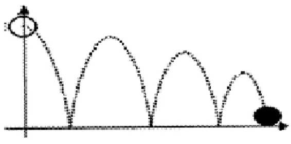
Example 5 (A Bouncing ball [9; 48; 93]) In this example, we consider a ball that is jumping on a ‡at horizontal surface (seeFigure 1). The loss of energy, caused by the friction of surface, is characterized by constant .

Figure 1 A Bouncing ball This process is simulated by a di¤ erential equation of second order

md

2_z

dt2 = F;

where m is the mass of the ball, F = mg, is the force (g 9:81m s2 is the acceleration of the Earth’s gravitation). Each time when the ball touches the ground the surface vertical component of the velacity vector changes its sign.

We consider a ball of mass m subject to the action of gravity. We let it fall from an altitude z0> 0 with a zero initial velocity. The altitude z(t) of the ball follows the di¤ erential equation

issued from the classical mechanics mz00(t) = mg; when z(t) = 0, the ball touches the ground and bounces loosing a fraction of its energy:

z00(t) = cz(t); with c 1:

Let us look what happens for the case of impulsive setting with the same bouncing ball. At time t0 we let the ball fall from an altitude z0 > 0. The variable of the system is x = (x1; x2), where

x1 is the altitude of the ball and x2 its velocity. The initial condition of the impulsive system

is (t0; (z0; 0)). As long as the altitude of the ball is positive one has

x0₁(t) = x2(t) and x 0 2(t) = g =) x2(t) = g(t t0) and x1(t) = g 2 (t t0) 2_{+ z} 0:

time t1 such that x1(t1) = 0; and so t1 = t0+ r 2z0 g ; x2(t1) = p 2gz0:

At this moment, the ball bounces:

x2(t+1) = cx2(t1) = c

p 2gz0:

Let tk be the moment when occurs the kth bouncing. Until the next impact of the ball on the

ground, one has

x2(t) = g(t tk) + x2(t+k) and x1(t) =

g

2 (t tk)

2_{+ x}

2(t+k)(t tk):

At time tk+1; the ball touches the ground

x1(tk+1) = 0 =) tk+1= tk+ 2 gx2(t + k); and boumces x2(t+_k+1) = cx2(t_k+1) = cx2(t+_k) = ::: = ckx2(t+1) = ck+1 p 2gz0:

Thus, the impulsive system admits an in…nite impulsion and the necessary time to attain the rest position is T = k=1_X k=0 (tk+1 tk) = r 2z0 g + k=1_X k=1 2 gx2(t + k) = r 2z0 g + k=1_X k=1 ck2 r 2z0 g ; if c < 1: Therefore, k=1_X k=0 (tk+1 tk) = r 2z0 g (1 + 2c 1 c) = T < 1:

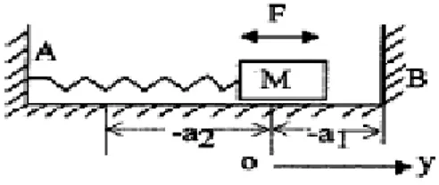
Example 6 [09; 13; 100] A body attached by a spring to a …xed point

A body M attached by a spring to a …xed point A and excited by a force F = h sin(pt + ), vibrates along a horizontal line and collides with a rigid wall B as shown in Fig. 2

Figure 2. A body M attached by a spring to a …xed point. The system can be described by the impulsive di¤ erential equations as follows

my00+ cy0_{+ ky = h sin(pt + ); y 2 [ a}2; a1] ; y0+= 8 < : y0; y = a1; y0 2 (0; b1] ; 2 (0; 1] ; y0; y = a1; y 0 2 [ b2; 0) ;

where y0+ is the velocity of the body after the impact is applied, y0 = 0 for y = a2; and all the

constants are positive.

A multi-body system vibrating with impact is given by

N y00+ Cy0+ Ky = H sin(pt + ); gi t; y; y0 6= 0;

y0+= By0; gi t; y; y

0

= 0; i = 1; 2; :::;

where y 2 Rn; N; C; K and B 2 Rn Rn; N; K are positive de…nite matrices and C is nonneg-ative de…nite matrix.

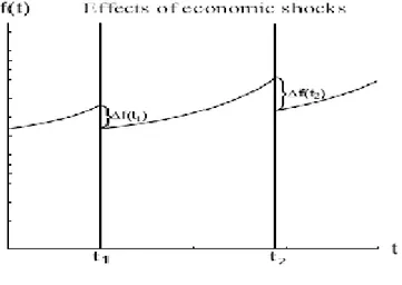
The results in this example are applicable to economic problems. Example 7 [41]The Impulsive Solow equation.

The seminal di¤ erential equation of Solow (1956) becomes an impulsive di¤ erential equation, when shocks to capital intensity are modelled with jumps. This statement results from an

analy-sis of unit roots in four German macroeconomic time series. IDE modelling of the Solow equation

Model the jumps of German capital K(t) and the capital intensity r(t) = K(t)

L(t) with real-valued piecewise continuous functions.

Let t1; t2; :::; tk::: > 0 be the moments, when the stock of capital K(t) is subject to shock e¤ ects

changing from the positions K(t_k) into the position K(t+_k) and r(t) is intrinsic to the system itself. An adequate mathematical model of the growth of capital in this case will be the impulsive di¤ erential equation of the form:

8 > > > < > > > : _ K(t) = sF (K(t); L0ent); t > t0; t 6= tk K(t0+ 0) = K0; K(t) = Jk(K(tk)) t = tk k = 1; 2; 3; :::; (1.1)

where functions Jk characterize the magnitude of the impulse e¤ ect at times tk; K(t0 0) and

K(t0+ 0) are respectively the capital level before and after the impulsive e¤ ect, K0 is the initial

capital.

Figure 3: Appearance of economic shocks in macroeconomic variables

It can be used in the economic studies of business cycles in situation when the total stock of capital K(t) is subject to shock e¤ ects.

problems of economics - the problem of the optimal control of the business cycles , (see R. M. May, [83]).

In the model (1.1) the moments of impulse e¤ ect is caused by an interior e¤ ect. But the moments of impulse e¤ ect can be caused by an exterior e¤ ect.

The solution of the impulsive Solow equation is the following K(t) = L0ent h r (t0)1 s n e n(1 )t₊ s n i 1 1 + X t0 tk<t Jk(K(tk)) :

The impulsive di¤erential equations can be successfully used to the mathematical simulation of biotechnological processes as seen in the following

Example 8 [12] Consider the equation of Verhulst dN

dt = N

k (K N ) ;

where N = N (t) denotes the biomass of a given population at the moment t 0, K is the capacity of the environment and is the di¤ erence between the birth-rate and death-rate. The case when external disturbances act upon the population is often met. We shall consider the cases when the external disturbances take place at …xed moments of time and are expressed as adding to or taking o¤ certain quantities of biomass. The impulsive analogue of the equation of Verhulst in this case has the form

8 > < > : dN dt = N k (K N ) t 6= tk N (tk) = N t+k N tk = Ik k = 1; 2; :::

where 0 < t1 < t2< t3< ::: are the moments of external e¤ ect, Ik; k = 1; 2; ::: are the amounts

of biomass added to (Ik < 0) or taken o¤ (Ik> 0) at the moments t1; t2; t3; :::

Impulsive di¤ erential equations arise naturally in various …elds such as population dynamics and optimal control. It seems that the …rst treatment of impulsive systems goes back to the monograph by Krylov and Bogolyubov [64] :

Example 9 [15](Population Dynamics ) The impulsive boundary value problem 8 > > > > > > > < > > > > > > > : @u @t(x; t) u(x; t) = u(x; t) a bu 2_{(x; t) ;} u( ; t) = 0; on in (0; T ); _{t 6= t}k; @ (0; T ); u(x; t+_k) = (1 + k)u(x; tk); on ftkg ; t = tk; u(x; 0+) = u0(x); on _{f0g ; k = 1; 2; ::::}

describes a single species population in bounded environment. The function y(x; t) represents the population density at the point x 2 and time t 0: Condition u(x; t+_k) = (1 + k)u(x; tk);

describes instantaneous changes in the population density due to phenomena as: harvesting, disasters, immigration, etc.

Example 10 [72] In this example, we assume that the host population is in a stationary de-mographic state, whose total size is constant N . Let N (a) ; 0 a rm (rm denotes the highest

age attained by the individuals in the host population) be the age density of the total number of individuals, and N (a) satis…es

N (a) = N e R0a (s)ds;

1(a) is the instantaneous death rate at age a of the host population, is the crude death rate,

we assume that (a) is nonnegative, locally integrable on [0; rm) ; and satis…es

Z rm 0 (a)da = 1; satis…es Z rm 0 f (a)da = 1;

where f (a) = e R0a (s)ds is the survival function. We can get the relation N (a) = N f (a).

The host population is divided into two groups: susceptible S(a; t) (who are healthy but can be infected), infected I(a; t) (which includes latent individuals, since individuals in incubation period can also infect susceptible population), S(a; t); I(a; t) is the age-densities of respectively

the susceptible and infected population at time t. N (a) also satis…es N (a) = S(a; t) + I(a; t):

Let M (t) denote the number of susceptible vectors (mosquito population) at time t; P (t) the number of infected vectors at time t: b; ₂ is the birth and death rate of vectors, respectively. Since blood transfusion, or using contaminated needles and syringes, susceptibles S(a; t) can be infected, and become infected individuals at a transmission ₁(a): Susceptibles S(a; t) are infected by infected vectors, and go into infected class at a transmission rate ₂: The number of new vectors by infected hosts depend on the transmission rate (a): The infected population can recover, and go into susceptible population at a transmission rate : In order to control the size of mosquito, we apply the pulse spraying strategy of insecticides, We spray insecticides upon mosquito at time n every months, is the period of spraying, n is the time at which we apply the nth_{(n 2 N ) pulse, and n} is the time just before applying the nth pulse. Every pulse can reduce a function p of mosquito population. We obtain the following system of equations that describes the dynamics of the model :

8 > > > > > > > > > > > > > > > > > > > > > > > > > > < > > > > > > > > > > > > > > > > > > > > > > > > > > : @S @t + @S @a = 1(a) + Rrm

0 1(a)I(a; t)da + 2p (t) S(a; t) + I;

for 0 < a < rm; t 6= n ; n 2 N ;

S(a; n ) = S(a; n _{); for t = n ; n 2 N ;} @I

@t + @I @a =

Rrm

0 1(a)I(a; t)da + 2p (t) S(a; t) ( 1(a) + ) I;

for 0 < a < rm; t 6= n ; n 2 N ;

I(a; n ) = I(a; n ); for 0 a < rm;

dM

dt = b M Rrm

0 (a)I(a; t)da 2M; for t 6= n ; n 2 N ;

M (n ) = (1 p) M (n _{) ; for t 6= n ; n 2 N ;} dP

dt = M Rrm

0 (a)I(a; t)da 2P; for t 6= n ; n 2 N ;

P (n ) = (1 p) P (n _{) ; for t 6= n ;} with boundary conditions

and initial conditions

S(0) = S0(a) 0; I(a; 0) = I0(a) 0; M (0) = M0 0; P (0) = P0 0;

where S0(a); I0(a) 2 L (0; rm) :

Chapter 2

Existence and Uniqueness Results

for Impulsive Evolution Equations

The problem of existence and uniqueness of the solution of impulsive evolution equations is similar to that of the corresponding ordinary evolution equations. The linear impulsive evolution equations in a Banach space have, for the …rst time, been considered by D. D. Bainov [12 15]. The existence of solutions, classical and mild, are established by Hernandez [54; 55], J. H. Liu, [78], Y. V. Rogovchenko [94], W. Zhang, R. P. Agarwal, E. Akin-Bohner [116], Chen Fangqi, chen Yushu [43], Benchohra [20; 21; 24] and Lakshmikanthan, [67] for linear and nonlinear cases. In this chapter, we present some basic properties of the impulsive problem in a Banach space. For more details one may refer to Hernandez [54; 55] and J. H. Liu [78] : We construct a new impulsive evolution operator corresponding to the impulsive evolution system and introduce a suitable de…nition of a PC-mild solution. The impulsive evolution operator can be used to reduce the existence of PC-mild solution for nonhomogeneous linear impulsive system to the existence of …xed points for some operator equation.

2.1 First order impulsive Cauchy problem

We de…ne impulsive di¤erential equations at …xed moments (…xed impulses) as follows: 8 > > > < > > > : y0(t) = Ay(t) + f (t; y); _{t 2 (0; T )}/_ftkg_k2 m 1 ; y(0) = y0;

y(t+) y(t ) = y(t ) = I y(t _{); k 2} m_;

where the …nal time T is a positive number, y0 is an initial condition in a Banach space X, endowed with a norm k:k, y : [0; T ] ! X is a vector function, and …nally, ftkg_k2 m

1 is an

increasing sequence of numbers in the open interval (0; T ) ; and y (tk) denotes the jump of

y (t) at t = tk

y (tk) = y t+k y tk ;

where y t+_k and y t_k represent the right and left limits of y (t) at t = tk; respectively: On the

other hand, the operators A; Ik : H ! H are given linear bounded or unbounded operators.

The function f : [0; T ] X _{! X is continuous on every closed interval [t}k; tk+1] ; and it is

non-linear in general.

The corresponding homogeneous system plays an important role in controllability studies, 8 > > > < > > > : '0(t) = A'(t); _{t 2 (0; T )} / ftkg_k2 m 1 ; '(0) = '0_; ' jt=tk = Ik('(tk)); k 2 m 1 ; (2.2)

and the following linear homogeneous impulsive di¤erential system 8 > > > < > > > : ~ '0 = A (t)~'; _{t 2 (0; T )}/_ftkg_k2 m 1 ; ~ '(0) = ~'0; ~ '(tk) = (I + Ik) 1Ik'(t~ k); k 2 m1 ;

is called the adjoint system to the impulsive system (2.2).

In the next section, we give some abstract results, some basic properties as well as the notion of solutions for the impulsive evolution equations.

Notion of Solution for the Impulsive Evolution Equation :

We …rst give the de…nition of a classical solution for impulsive evolution equations.

De…nition 11 (Classical solution) By a classical solution of an impulsive evolution equation we mean a piecewise absolutely continuous mapping with discontinuities of …rst kind at the points t = tk which, for almost all t; satis…es the system (2.1) and for t = tk, satis…es the jump

condition. In other words, a classical solution of the impulsive equation (2.1) is a function y 2 PC([0; T ] ; X) \ C1((0; T )/_{ft g ; X ); y(t) 2 D(A); for t 2 (0; T ) nft g}m; such that y

satis…es (2.1) in [0; T ) :

Note that the classical solutions for evolution equations without impulsive conditions are de…ned in an obvious way, see Pazy [90].

To be able to apply the method in [90], we need the following lemmas. Lemma 12 [90] Consider the evolution problem

8 < :

y0_{(t) = Ay(t) + f (t; y); t 2 (0; T ) ;} y(0) = y0:

If y0 _{2 D(A), and f 2 C}1((0; T ) X; X), then it has a unique classical solution which satis…es y(t) = S(t)y0+R₀tS(t _{s)f (s; y(s))ds; t 2 [0; T ) ;}

where S(t) is the semigroup generated by A:

Lemma 13 [78] Let assumptions (H1)-(H2) be satis…ed, and assume that y0 _{2 D(A) and} that f 2 C1_{((0; T ) X; X). Then, for the unique classical solution y(:; y}0_{) on [0; t}

1) of system

(2.1) without impulses (guaranteed by Lemma 12), one can de…ne y(t1) in such a way that y

is left continuous at t1 and y(t1) 2 D(A):

Proof. Consider the following evolution problem without impulses in (0; T ), 8

< :

w0(t) = Aw(t) + f (t; w(t)); 0 < t < T; w(0) = y0;

From Lemma 12, there is a classical solution given by

w(t) = S(t)y0+R₀tS(t _{s)f (s; w(s))ds; t 2 [0; T ) ;}

with w(t) 2 D(A); for t 2 [0; T ) : Next, applying Lemma 12 one has, for t 2 [0; t1) [0; T )

Next, we de…ne

y(t1) = S(t1)y0+

Z t1

0

S(t1 s)f (s; y(s))ds;

so that y(:) is left continuous at t1. Then apply Lemma 12 in [0; t1] to get

y(t) = w(t); [0; t1]:

Thus, we have, y(t1) = w(t1) 2 D(A) which completes the proof.

Before proving the main theorem, we need the following Lemma.

Lemma 14 [78] Assume that y0 _{2 D(A); q}k2 D(A); k 2 m1 and that f 2 C1((0; T ) X; X).

Then the impulsive system 8 > > > < > > > : y0_{(t) = Ay(t) + f (t; y(t)); t 2 (0; T )}/_ftkg_k2 m 1 ; y(0) = y0; y(tk) = qk; k 2 m1 ; (2.3)

has a unique classical solution y which, for t 2 [0; T ) ; satis…es y(t) = S(t)y0+ Z t 0 S(t s)f (s; y(s))ds + X 0<tk<t S(t tk)qk: (2.4)

Proof. First consider the interval J1= [0; t1) and apply Lemma 12 to the equation

y0(t) = Au(t) + f (t; y(t)); 0 < t < t1; y(0) = y0:

We obtain a unique classical solution y1 satisfying

y1(t) = S(t)y0+ Z t 0 S(t s)f (s; y1(s))ds; t 2 [0; t1) ; Next, de…ne y1(t1) = S(t1)y0+ Z t1 0 S(t1 s)f (s; y1(s))ds;

hand in J2 = [t1; t2), consider the equation

y0(t) = Au(t) + f (t; y(t)); t1 < t < t2; y(t1) = y1(t1) + q1

Since y(t1) = y1(t1) + q1 2 D(A); we can once again use Lemma 12 to get a unique classical

solution y2 satisfying y2(t) = S(t t1) [y1(t1) + q1] +R_tt₁S(t s)f (s; y2(s))ds; t 2 [t1; t2); so that y2(t2) = S(t2 t1) [y1(t1) + q1] + Z t2 t1 S(t s)f (s; y2(s))ds:

Therefore, y2(:) is left continuous at t2 and y2(t2) 2 D(A). It is easily seen that this procedure

can be repeated in Jk= [tk 1; tk); k 2 m+13 to get a classical solution

yk(t) = S(t tk 1) [yk 1(tk 1) + qk 1] +

Rt

tk 1S(t s)f (s; yk(s))ds; t 2 [tk 1; tk) ;

with yk(:) left continuous at tk and yk(tk) 2 D(A); k 2 m1 :

Now, de…ne y(t) = 8 > > > < > > > : y1(t); 0 < t < t1; yk(t); tk 1 < t < tk; k 2 m2 ; ym+1(t); tm < t < T:

It is clear that y(:) is the unique impulsive classical solution of (2.3).

Next, we use induction to show that (2.4) is satis…ed in [0; T ). In fact, (2.4) is satis…ed in [0; t1]. If (2.4) is satis…ed in (tk 1; tk], then for t 2 (tk 1; tk]

y(t) = yk+1(t) = S(t tk) [yk(tk) + qk] + Z t tk S(t s)f (s; y(s))ds = S(t tk) S(tk)y0+ Z t tk S(tk s)f (s; y(s))ds + X 0<ti<tk S(tk ti)qi+ qk 3 5 +Z t tk S(t s)f (s; yk+1(s))ds

y(t) = S(t tk)T (tk)y0+ Z tk 0 S(t s)f (s; y(s))ds + X 0<ti<tk S(t ti)qi +S(t tk)qk+ Z t tk S(t s)f (s; y(s))ds = S(t)y0+ Z t 0 S(t s)f (s; y(s))ds + X 0<ti<t S(t ti)qi:

Thus (2.4) is also true on (tk; tk+1]. Therefore (2.4) is true on [0; T ).

In what follows, we study the existence and uniqueness of mild solutions using the …xed point argument. First we start with the de…nition.

De…nition 15 (Mild solution) _{A function y(:) 2 PC([0; T ] ; X) \ C}1((0; T ) /

ftkg_k2 m 1 ; X );

is a mild solution for the problem (2.1) if it satis…es the impulsive condition and y(t) = S(t)y0+ Z t t0 S(t s)f (s; y(s))ds + X t0<tk<t S(t tk)Iky(tk); 8t 2 [0; T ) : (2.5)

We assume the following hypotheses:

(H1) f : [0; T ] _{X ! X and I}k : X ! X; k = 1; ::m; are continuous and there exist

constants L(f ) > 0; L(Ik) > 0; k 2 m1 ; such that

f (t; x) f (t; x0) L(f ) x x0 _{; t 2 [0; T ] ; x; x}0 _{2 X} Ik(x) Ik(x 0 ) L(Ik) x x 0 ; x; x0 _{2 X:}

(H2) Let S(:) be the strongly continuous semigroup generated by the unbounded

operator A: Let L(X) be the Banach space of all linear and bounded operators on X. We suppose that M " L(f )T + m X k=1 L(Ik) # < 1; where M = sup t2[0;T ]kS(t)kL(X) :

Under these assumptions, we can establish the existence and uniqueness of mild solutions. Theorem 16 [78] Let assumptions (H1)-(H2) be satis…ed. Then for every y0 _{2 D(A), the} problem (2.1) has a unique mild solution.

Proof. Let y0_{2 X be …xed. De…ne the operator F on PC([0; T ] ; X) by} (F x)(t) = S(t)y0+ Z t 0 S(t s)f (s; x(s))ds + X 0<tk<t S(t tk)Ikx(tk);

Then, it is clear that F : PC([0; T ] ; X) ! PC([0; T ] ; X). On the other hand, we have from assumption (H1), k(F x)(t) (F z)(t)k Z t 0 kS(t s)kL(X)kf(s; x(s)) f (s; z(s))k ds + X 0<tk<t kS(t tk)k_L(X)kIkx(tk) Ikz(tk)k M LT kx zk_PC+ X 0<tk<t M hkkx(tk) z(tk)k M LT kx zk_PC+ M kx zk_PC X 0<tk<t hk M " LT + k=m_X k=1 hk # kx zk_PC; x; z 2 PC([0; T ] ; X):

Now from assumption (H2), we see that F is a contraction operator on PC([0; T ] ; X). We conclude by the …xed point theorem that there is a unique mild solution y 2 PC([0; T ] ; X) such that

y = F y: This completes the proof.

Next, we study the existence of mild solutions for the initial value problem (2.1) We set the following assumptions:

(A1) _{The function a : [0; T ] ! [0; T ] is continuous and a(t) t; for every t 2 [0; T ] ;} (A2) The function f : [0; T ] X2 _{! X;}

satis…es the Caratheodory condition i.e.

(a) f (t; :) : X ! X is continuous for almost all t 2 [0; T ] ; (b) f (:; x) : [0; T ] 7 ! X is integrable for each x 2 X;

and there exists a continuous function g : [0; T ] ! [0; 1) and a nonincreasing function W : [0; 1) ! [0; 1) ;

such that

kf(t; x; y)k g(t)W (kxk + kyk); for all t 2 [0; T ] and x; y 2 X:

Theorem 17 [55] Let y0 _{2 X and let the following assumptions hold.}

(1) For each k 2 m1 , the operator Ik is completely continuous and bounded in X; with

Nk= sup fkIk(x)k : x 2 Xg ;

(2) For every t 2 [0; T ] and r > 0 the region fS(t)f(s; x1) : s 2 [0; t] ; kx1k r; g is relatively

compact in X. If 2M T R 0 g(s)ds < 1_R c ds W (s); where c = 2(M ku0k +Pnk=1M Nk); and M = sup t2[0;T ]kS(t)k ;

then the problem (2.1) has a unique mild solution. Remark 1

(1) If y is a solution of (2.1) then y 2 PLC1([0; T ] ; X):

(BV ((0; T ); X) being the space of bounded variation functions) and y(t) = S(t)y0+R₀tS(t s)f (s; y(s); )ds + X

0<tk<t

S(t tk)Ik(y(tk)); 8t 2 [0; T ] :

In fact, it has two parts: the …rst part is a continuous function yc 2 W1;1(0; T ; X), with

yc(t) = S(t)y0;

while the second one is the jump function de…ned by yd(t) =

X

0<tk<t

S(t tk)Ik(y(tk)); 8t 2 [0; T ] :

(3) The problem of existence and uniqueness of the solutions of impulsive di¤ erential equations is similar to that of the corresponding ordinary di¤ erential equations. We can represent the solution y(t) of equation (2.1) with initial condition y(0) = y0; as follows,

y(t) = 8 > > < > > : S(t)y0+R_tt 0S(t s)f (s; y(s))ds + P t0<tk<t S(t tk)Iky(tk); t 2 [t0; T ]+; S(t)y0+R_tt 0S(t s)f (s; y(s))ds P t0<tk<t S(t tk)Iky(tk); t 2 [t0; T ]

where [t0; T ]+ and [t0; T ] are maximal intervals on which the solution can be continued to the

right or to the left of the point t = t0, respectively.

(4) As a result, the solution of (2.2) is given by

'(t) = S(t tk)'(tk); for t 2 [tk; tk+1) ; k = 0; 1; 2:::

(5) The relationship between nonhomogeneous equation (2.1) and the corresponding homoge-neous equation is the following: if '(t) is a classical solution of (2.2) without an initial condition and y(t) is a classical solution of (2.1) without an initial condition, then the function '(t) + y(t) is again a classical solution of (2.1) without initial condition. Conversely, if y1(t) and y2(t) are

two solutions of (2.1) without an initial condition, then the di¤ erence y1(t) y2(t) is a solution

(6) If Ik = 0 for k 2 m1 ; then the equation (2.2) reduces to the ordinary evolution equation 8 < : '0_{(t) = A'(t); t 2 (0; T )}/_ftkg_k2 m 1 ; '(0) = '0; and the solution (2.2) reduces to

'(t) = S(t)'0:

Regarding the solution of (2.2), we have the following result.

Theorem 18 [80] If Ik maps D(A) to D(A), k = 1; 2::: and '0 2 D(A); then problem (2.2)

has a unique solution '(t) given by

'(t) = 8 > < > : S(t)'0 0 t t1 S(t)'0+ k P i=1 S(t ti)Ii('(ti)); tk< t tk+1; k 2 m0 : (2.6)

Proof: It follows from A.Pazy; [89] that the function '(t) de…ned by (2.2) satis…es (2.2)1

for 0 < t t1 and '(t1) = S(t1)'0 = '(t1) and such a solution '(t) is unique. From the given

assumption, we have '(t1) = I1('(t1)) 2 D(A): If '(t); de…ned by (2.2), satis…es equation

(2.2)1 for ti < t < ti+1, i 2 k1 and

'(t_i+1) = '(ti+1) = S(ti+1)'0+ i

P

j=1

S(ti tj)Ij('(tj)); i 2 k1;

'(ti) = Ii('(ti)) 2 D(A); i 2 k1;

then, for tk+1< t < tk+2; we have

'0(t) = AS(t)'0+ k+1_P i=1 AS(t ti)Ii('(ti)) = A'(t); '(t_k+2) = '(tk+2) = S(tk+2)'0+ k+1_P i=1 S(ti+1 ti)Ii('(ti));

and '(tk+1) = '(t+k+1) '(tk+1) = S(tk+1)'0+ k+1_P j=1 S(tk+1 tj)Ij('(tj)) S(tk+1)'0+ k P j=1 S(tk+1 tj)Ij('(tj)) = Ik+1('(tk+1)) 2 D(A):

Thus, the theorem is proved by induction.

Example 19 Let ; k 2 R; k 2 m1 and k 6= 1 for every k 2 m1 : Then, the solution

' 2 PLC [0; T ] ; ftkg_k2 m 1 ; X of 8 > > > < > > > : '0(t) + '(t) = 0 _{(0; T ); t 6= tk}; _{k 2} m₁ ; '(t+_k) = (1 + k)'(tk) '(0) = '0: is given explicitly by '(t) = Q 0<tk<t (1 + k)'0:

The next result is a consequence of Theorem 2.4. Impulsive Partial Di¤erential Equations Consider the partial di¤erential problem :

8 > > > < > > > : @y(x; t) @t + a(x) @y(x; t) @x = f (x; y); t > 0; t 6= tk; k 2 m 1 x 2 R; y(x; 0) = (x); y(x; tk) = Ik(y(x; tk)); k 2 m1 (2.7)

where Ik 2 C(Y; Y ); and

Y = C0(R) 2 C(R) : lim

with norm

k k = sup

x2Ij (x)j :

We de…ne the operator A on Y as follows :

A(x) = a(x)d (x)

dx ; (2.8)

D(A) = _{2 Y :} 0(x) exists and is continuous at x; lim

jxj!+1a(x) (x) = 0;

lim

x!x0

a(x) (x) exists when a(x0) = 0 :

We set the following assumptions :

(i) a(x) is positive and continuous on R; (ii) R₀1( 1

a(x))dx = +1 andjxj!+1lim a(x) = 0;

(iii) f 2 C1(R R); there exist a real positive number M such that @f (x; u)

@x M and

@f (x; u)

@u M; for every (x; u) 2 R R; limx! 1f (x; u) = 0; for each u 2 R;

(iv) Ik2 L(X) and Ik(D( A)) D( A):

Next, we are going to discuss the existence of solutions for the …rst order impulsive evolution problem (2.7).

Theorem 20 [80] Suppose (i)-(iv) are satis…ed. Then problem (2.7) has a unique mild solution in [0; 1) :

Proof: First, problem (2.7) can be written in an abstract form, 8 > > > < > > > : y0_{(t) + Ay(t) = g(y(t)); t 6= t}k; y(0) = y0; y jt=tk = Ik(y(tk)); k 2 m 1 ; (2.9)

(t) = 8 < :

S(t); [0; t1]

S(t tk)(Ik+ I)S(tk tk 1):::(I1+ I)S(t1); (tk; tk+1] ; k = 1; 2:::;

where S(t) is the semigroup generated by A:

Taking y1(t) = y0; then g(y1(t)) 2 D( A) and (t)g(y1(t)) is continuous in t except at tk;

it has discontinuities of …rst kind at tk and it is integrable in t: Hence, we can de…ne

u2(t) = (t)y0+ Z t 0 (t; )g(y1( ))d ; where (t; ) = 8 > > > > > > > > > > > > < > > > > > > > > > > > > : S(t tk)(Ik+ I)S(tk tk 1)::: :::(I1+ I)S(t1 ) S(t tk)(Ik+ I)S(tk tk 1)::: if t 2 (tk; tk+1] ; 2 [0; t1]

:::(Il+ I)S(tl ); if k l and t 2 (tk; tk+1] ; 2 (tl 1; tl] ;

S(t ); if t and t; _{2 (t}k; tk+1]

or t; _{2 [0; t}1] ; k = 1; 2:::; l = 1; 2::::

It is easy to check that y2(t) 2 D( A); if t 6= tk; and satis…es the following problem:

8 > > > < > > > : w0(t) + Aw(t) = g(y1(t)); t 6= tk; k = 1; 2:::; w(0) = y0; w jt=tk = Ik(w(tk)); k = 1; 2::::

In a similar way, we can de…ne

yn(t) = (t)y0+

Z t 0

for n = 2; ::::; so that yn(t) satis…es 8 > > > < > > > : w0(t) + Aw(t) = g(yn 1(t)); 0 < t < 1; t 6= tk; w(0) = y0; w jt=tk = Ik(w(tk)); k = 1; 2::: (2.11)

For a given T > 0; let k0= max fk jtk2 [0; T ]g and N = max fkIkk jkIkk 1; and 1 k k0g ;

we get kyn+1(t) yn(t)kY N M Z t 0 ky n( ) yn 1( )kY d ; for n = 2; 3; :::: Therefore, kyn+1(t) yn(t)kY (N M ) n 1 tn 1 n! 0maxSky2( ) y1( )k ; (2.12)

for n = 2; 3; ::::It follows from (2.12) that there exists a real valued function y(t) on [0; T ] such that yn(t) converges uniformly to y(t) on [0; T ] : Since yn(t) satis…es (2.11), then by virtue of

(2.10) and assumption on f; we see that y(t) satis…es y(t) = (t)y0+

Z t 0

(t; )g(y( ))d :

The argument above shows that (2.9) has a mild solution on [0; T ] ; for each T > 0: If the problem (2.9) has another mild solution ~y(t) on [0; T ] ; then

ky(t) _y(t)k~ _Y M Z t

0 k (t; )k ky(t)

~

y(t)kY d :

By Gronwall’s inequality, y(t) = ~y(t) on [0; T ] : So, we see that problem (2.9) has a unique global mild solution on [0; 1) : The theorem is proved.

Representation of Solutions of Some Impulsive Linear Systems

This section deals with the solution representation of linear impulsive evolution equations. We consider the following homogeneous linear impulsive system with time-varying

generat-ing operators ₈ > > > < > > > : y0_{(t) = A(t)y(t) + f (t); t 2 (0; T )}/_ftkg_k2 m 1 ; y(0) = y0; y(tk) = Iky(tk) + k; k 2 m1 ; (2.13)

on some in…nite dimensional Banach space X; where 0 = t0 < t1 < t2 < :::: < tk::: < tm <

T; and fA(t); t 2 [0; T ]g is a family of unbounded operators on X satisfying the following assumptions :

For t 2 [0; T ] one has

(H1) The domain D(A(t)) = D is independent of t and is dense in X: (H2) A(t) is a closed operator in X:

(H3) For t 0; the resolvent R( ; A(t)) = ( I A(t)) 1 exists, for all with Re 0; and there exists a real constant M independent of and t such that

kR( ; A(t))k M (1 + j j) 1 for Re 0: (H4) The resolvent of the unbounded operator A(t) is compact. (H5) There exist constants L > 0 and 0 < 1 such that

(A(t) A(s)) A 1(r) _{L jt sj ;} for _{t; s; r 2 [0; T ] :} Let us begin with the following lemma.

Lemma 21 (See Ahmed [2] p. 159) Under assumptions (H1)-(H5), the Cauchy problem x0_{(t) = A(t)x(t); t 2 (0; T ] with x(0) = x}0; (2.14) has a unique evolution system fU(t; s) j 0 s t _{T g in X satisfying the following properties} (1) U (t; s) 2 L(X); for 0 s t T:

(2) U (t; r)U (r; s) = U (t; s); for 0 s t T:

(3) U (:; :)x 2 C ( T; X) ; for x 2 X; T = f(t; s) : s 2 [0; T ] ; t 2 [s; T ]g :

derivative @

@tU (t; s) 2 L(X) and it is strongly continuous on 0 s < t T: Moreover, @ @tU (t; s) = A(t)U (t; s); for 0 s < t T; @ @tU (t; s) _L(X)= kA(t)U(t; s)kL(X) C t s; A(t)U (t; s)A 1_(s) L(X) C; for 0 s < t T:

(5) For every z 2 D and t 2 (0; T ] ; U(t; s)z is di¤erentiable with respect to s on 0 s t T and

@

@sU (t; s)z = U (t; s)A(s)z:

Furthermore, for each x0 _{2 X; the Cauchy problem (2.14) has a unique classical solution} x 2 C1([0; T ] ; X) given by

x(t) = U (t; 0)x0_{; t 2 [0; T ] :}

In order to construct an impulsive evolution operator and investigate its properties, we shall consider the following impulsive Cauchy problem

8 > > > < > > > : y0(t) = A(t)y(t); _{t 2 (0; T )}/_ftkg_k2 m 1 ; y(0) = y0; y(tk) = Iky(tk); k 2 m1 ; (2.15)

where m 2 N ; is a …xed positive integer. For every y0 2 X; D is an invariant subspace of Ik.

Using Lemma 1 and 2 in ([12] p. 19-20.) step by step, one can check that the impulsive Cauchy problem (2.15) has a unique classical solution y 2 PC([0; T ] ; X) \ C1((0; T )/_ftkg_k2 m

1 ; X );

G(t; s) = 8 > > > > > > > > > > > > > > > > > > > > > > > > > > > < > > > > > > > > > > > > > > > > > > > > > > > > > > > : Uk(t; s), for s t 2 [tk 1; tk] ; Uk+1(t; t+k) (I + Ik) Uk(tk; s); for tk 1 < s tk < t tk+1; k 2 m1 ; Uk(t; tk) (I + Ik) 1Uk+1(t+k; s); for tk 1< s tk< t tk+1; k 2 m1 ; Uk+1(t; tk) 2 4 i+1 Y j=k (I + Ij) Uj(tj; t+j 1) 3 5 (I + Ii) Ui(ti; s); for ti 1< s ti < tk< t tk+1; k 2 m1 ; Ui(t; ti) 2 4 k 1_Y j=i (I + Ij) 1Uj+1(t+j; tj+1) 3 5 (I + Ik) 1Uk+1(t+_k; s); for ti 1< t ti< tk< s tk+1; k 2 m1 :

The operator G(t; s); (t; s) 2 T is called the impulsive evolution operator associated with

fIk; tkg_k2 m 1 :

Proposition 22 _{[105] The impulsive evolution operator G(t; s); (t; s) 2} T has the following

properties:

(a) G(t; s) 2 L(X) for 0 s t T:

(b) G(t; r)G(r; s) = G(t; s) for 0 r s t T; and G(s; s) = I:

(c) If fU(t; s)g 0 s < t T is a compact operator, then G(t; s) is also compact for 0 s < t T:

Proof : (a) is due to property (1) of Lemma 21 and assumption Ik2 L(X) for k 2 m1 ;

(b) is evident,

(c) Since fU(t; s)g ; 0 s < t T are compact operators, one can deduce that G(t; s) is also compact for 0 s < t T:

Now we are able to introduce the PC mild solution of impulsive Cauchy problem (2.13) as follows :

De…nition 23 For every y0_{2 X; f 2 L}1_{([0; T ] ; X); the function y 2 PC((0; T )}/_ftkg_k2 m 1 ; X )

given by x(t) = G(t; 0)x0+ Rt 0G(t; s)f (s)ds + X 0<tk<t G(t; t+_k) k; for t 2 [0; T ] :

is said to be a mild solution of the impulsive Cauchy problem (2.13). On the other hand, we have the following existence theorem :

Theorem 24 _{[49] If fU(t; s)g ; t; s 2} T is an evolution operator in a Banach space X with

in…nitesimal generator A (t) and Ik2 L(X); for k 2 m1 ; then the problem

8 > > > < > > > : y0_{(t) = Ay(t) + f (t); t 2 (0; T ) t 6= t}k; k 2 m1 ; y(0) = y0; y(tk) = Ik(y(tk)); k 2 m1 ; (2.16)

has a unique solution y(t) given by y(t) = U (t; t+_{k 1})y(t+_{k 1}) +R_tt k 1U (t; s)f (s)ds; t 2 (tk; tk+1] ; k 2 m 1 ; (2.17) such that y(t+_k) = 1 Y j=k (I + Ij) U (tj; tj 1)y0+ k X i=1 i Y j=k (I + Ij) U (tj; tj 1) (2.18) Z ti ti 1 U (ti; s)f (s)ds; for each k 2 m1 : Proof : We have y0_{(t) = Ay(t) + f (t); t 2 [t}0; t1] ; y(0) = y0;

and the ordinary variation of parameters leads to y(t) = U (t; t0)y(t+0) +

Rt

y(t1) = U (t1; t0)y(t+0) +

Z t1

t0

U (t1; s)f (s)ds:

Since y(t1) = I1(y(t1)) ; then

y(t1) = (I + I1) U (t1; t0)y(t0) + (I + I1) U (t1; t0) Z t1 t0 U (t0; s)f (s)ds: (2.19) Moreover, for t 2 (t1; t2] ; y(t) = U (t; t1)y(t+₁) +R_tt 1U (t; s)f (s)ds; t 2 (t1; t2] ;

where y(t+₁) is given by (2.18). This implies that Theorem 24 holds for k = 1: Now, suppose that (2.16) and (2.17) are true when k = m; namely, as t 2 (tm; tm+1] ; one has

y(t) = U (t; tm)y(t+m) + Z t tm U (t; s)f (s)ds; (2.20) where y(t+_m) = 1 Y j=m (I + Ij) U (tj; tj 1)y0+ m X i=1 i Y j=m (I + Ij) U (tj; tj 1) (2.21) Z ti ti 1 U (ti 1; s)f (s)ds: then, (2.20) leads to y(t) = U (tm+1; tm)y(t+m) + Z tm+1 tm U (t; s)f (s)ds: It follows from the impulsive system (2.15) and (2.21) that

y(t+_m+1) = (I + Im+1) y(tm+1)

= (I + Im+1) U (tm+1; tm)y(t+m) +

Z tm+1

tm

y(t+_m+1) = (I + Im+1) U (tm+1; tm)y(t+m) + (I + Im+1) U (tm+1; tm) Z tm+1 tm U (tm; s)f (s)ds = (I + Im+1) U (tm+1; tm) 1 Y j=m (I + Ij) U (tj; tj 1)y0 + (I + Im+1) U (tm+1; tm) m X i=1 i Y j=m (I + Ij) U (tj; tj 1) Z ti ti 1 U (ti 1; s)f (s)ds + (I + Im+1) U (tm+1; tm) Z tm+1 tm U (tm; s)f (s)ds = 1 Y j=m+1 (I + Ij) U (tj; tj 1)y0+ m+1_X i=1 i Y j=m+1 (I + Ij) U (tj; tj 1) Z ti ti 1 U (ti 1; s)f (s)ds: Accordingly, as t 2 (tm+1; tm+2] ; we have y(t) = U (t; tm+1)y(t+m+1) + Z t tm+1 U (t; s)f (s)ds;

which means that (2.16) and (2.17) hold when k = m + 1: Then the Theorem is true for any t 2 (tk; tk+1] ; and k 2 m1 : This, completes the proof.

The next theorem is of theoretical importance as it relates the solutions of (2.13) with the impulsive evolution operator G(t; 0):

Theorem 25 [7] Let x(t) = x(t; 0; x0) be a solution of the impulsive problem (2.13). Then x(t)

has the representation

x(t) = G(t; 0)x0+ Z t 0 G(t; s)f (s)ds + X 0<tk<t G(t; t+_k) k where x(0) = x0; and t 0:

Proof. Let x(t; 0; x0) be the solution of (2.13) and let t(s) = G(t; s)x(s): Clearly,

(t) (0) = Z t 0 0 (s) ds + X 0<tk<t (tk) :

Since we have (tk) = G(t; t+k)x t + k G(t; tk)x tk = G(t; t+_k) x t+_k x t_k + G(t; t+_k)x t_k G(t; t_k)x t_k = G(t; t+_k) x (tk) + G(t; tk)x tk ; we obtain that X 0<tk<t (tk) = X 0<tk<t G(t; tk)x t_k + G(t; t+_k) x (tk) = X 0<tk<t G(t; tk)x tk + X 0<tk<t G(t; t+_k)Ikx tk + X 0<tk<t G(t; t+_k) k = X 0<tk<t G(t; tk)x t_k + X 0<tk<t [ G(t; tk) + G(t; tk)] Ikx t_k + X 0<tk<t G(t; t+_k) k = X 0<tk<t G(t; tk) [I + Ik] x tk + X 0<tk<t G(t; tk)Ikx tk + X 0<tk<t G(t; t+_k) k = [ G(t; tk) (I + Ik) + G(t; tk)Ik] x t_k + X 0<tk<t G(t; t+_k) k:

On the other hand, by di¤erentiating the relation (s) = G(t; s)x(s) we obtain

0

(s) = @

@sG(t; s) x(s) + G(t; s)x

0

(s)

Integrating both sides from 0 to t we get G(t; t)x(t) G(t; 0)x(0) = Z t 0 G(t; s)f (s)ds + X 0<tk<t [ G(t; tk) (I + Ik) + G(t; tk)Ik] x tk + X 0<tk<t G(t; t+_k) k: Thus, we obtain x(t) = G(t; 0)x(0) + Z t 0 G(t; s)f (s)ds + X 0<tk<t G(t; t+_k) k:

This completes the proof.

Suppose that X is a Hilbert space. Consider the following Cauchy problem 8 > > > < > > > : '0_{(t) + A(t)' (t) = 0; t 2 (0; T ) n ft}kg_k2 m 1 ; ' (0) = '0; ' (tk) = Ik' (tk) ; k 2 m1 : (2.22)

Consider the corresponding adjoint impulsive problem : 8 > > > < > > > : ~ '0(t) + A (t)~'(t) = 0; _{t 2 (0; T ) n ft}kg_k2 m 1 ; ~ '(T ) = '0; ~ '(tk) = Ik(I + Ik) 1_'(t~ k) k 2 m 1 ; (2.23)

where A (t) ; I_k are the adjoint operators of A (t) and Ik; respectively.

Remark 2 It is easy to verify also that the adjoint problem of (2.22) is (2.23), i.e. they are mutually adjoint of each other.

Similarly to the discussion on the adjoint impulsive Cauchy problem of homogenous linear impulsive system with time-varying generating operator, the mild solution of the impulsive

problem (2.23) can be given as ~ x( ) = (T; )~x0; < T; where (T; ) = 8 > > > > > > > > > < > > > > > > > > > : U (T; ); for _{2 (t}k 1; T ] ; U (tk 1; ) (I + Ik) U (T; tk 1); for tk 2< s tk 1< T; U (ti; ) (I + Ii) 2 4 Y <tJ<T (I + Ij) U (tj; tj 1) 3 5 U (T; tk 1); for ti 1< ti< tk< ::: < T:

The next theorem relates the solution of (2.23) with the impulsive evolution operator (T; ):

Theorem 26 [7] Let ~x( ) = ~x(T; ; ~x0) be a solution of the impulsive problem (2.25). Then

~

x(s) has the representation ~ x( ) = (T; )~x0+ Z T (s; )Bu(s)ds + X <tk<T (t_k; )Dkvk with ~ x(T ) = ~x0:

Proof. The proof is similar to that of Theorem 25. Let ~x(T; ; ~x0) be the solution of (2.23)

and let (s) = (s; )~x(s): Clearly, ( ) (T ) = Z T0 0 (s) ds + X <tk<T (tk)

Recall that (tk) = (tk; )~x tk (t + k; )~x t + k = (t_k; ) ~x t_k x t~ +_k + (t_k; )~x t+_k (t+_k; )~x t+_k = (t_k; ) x (t~ k) + (tk; )~x t+k ; Let Jk + Ik(I + Ik) 1_{; we obtain that} X <tk<T (tk) = X < k<T (tk; )~x t+_k + (t_k; ) x (t~ k) = X <tk<T (tk; )~x t+_k + (t_k; ) [Jk] ~x t+_k + (t_k; )D_kwk = X <tk<T (tk; )~x +k + (tk; ) + (tk; ) [Jk] ~x t+k + (t_k; )D_kwk = X < k<T (tk; ) [I + Jk] ~x t+k + X < k<T ( k; ) [Jk] ~x +k + X < k< ( _k; )D_kwk = X < k< ( k; ) [I + Jk] + ( k; ) [Jk] ~x +k + X <tk<T ( _k; )D_kwk:

On the other hand, by di¤erentiating the function (s) = (s; )~x(s) we obtain

0 (s) = d ds[ (s; )~x(s)] = @ @s (s; ) ~x(s) + (s; )~x 0 (s) = A G(t; s)x(s) + G(t; s) [A x(s)] + (s; )B u (s):

Hence ( ; )~x( ) (T; )~x(T ) = Z T (s; )B (s)ds + X <tk<T (tk; ) (I + Jk) + (tk; )Jk x t~ +k + X <tk<T (t_k; )D_kwk: Thus, we obtain ~ x( ) = (T; )~x(T ) Z T (s; )B (s)ds + X < k<T ( k; ) (I + Jk) + ( k; )Jk x t~ +_k + X < k<T ( _k; )D_kwk:

This completes the proof.

Proposition 27 [7] The impulsive evolution operators G(t; s) related to (2.22) can be repre-sented explicitly as follows

G(t; t) G(t; 0) = Z t 0 G(t; s)A (s) ds X 0<tk<t h Ik(I + Ik) 1 i G(t; t_k)

Proof. Let G(t; s) be an impulsive evolution operator of (2.22). Then, 8 > < > : @ @sG(t; s) = G(t; s)A (s) ; t 2 [tk; tk+1) ; k 2 m 0 ; + 2G(t; tk) = G(t; t+k) G(t; tk) = G(t; tk) h Ik(I + Ik) 1 i k 2 m 10 :

It is not di¢ cult to see that the integration of @

@sG(t; s) with respect to s over an interval [0; t] leads to G(t; t) G(t; 0) = Z t 0 G(t; s)A (s) ds X 0<tk<t h Ik(I + Ik) 1 i G(t; t_k):

This completes the proof.

Proposition 28 [7] The impulsive evolution operators (s; ) of (2.23) can be explicitly rep-resented as follows (T; ) = ( ; ) + Z T (s; )A (s) ds + X <tk<T h Jk(I + Jk) 1 i (tk; )

Proof. Let (s; ) be the impulsive evolution operators of (2.23). Then, 8 > < > : @ @s (s; ) = (s; )A (s) ; t 2 (tk; tk+1] ; k 2 m 0 ; 1 (tk; ) = h Jk(I + Jk) 1 i (tk; ); k 2 m 10 :

It is not di¢ cult to see that the integration of @

@s (s; ) with respect to s over an interval [ ; T ] leads to ( ; ) (T; ) = Z T (s; )A (s) ds + X <tk<T h Jk(I + Jk) 1 i (tk; ) which gives (T; ) = ( ; ) + Z T (s; )A (s) ds + X <tk<T h Jk(I + Jk) 1 i (tk; ):

This completes the proof.

A direct consequence of the Proposition 2.27 is the following. Corollary 29 [7] Let I +

h

Ik(I + Ik) 1

i 1

= Ik; k 2 m1 : For each s 2 [0; T ] we have

8 < : @ @tG(t; s) = G(t; s)A (t) ; t 2 [tk; tk+1) ; k 2 m 0 ; + 1G(tk; s) = G(t+_k; s) G(t_k; s) = IkG(t_k; s) k 2 m1 :

Proof. By Proposition 2.27 we have G(t; t) G(t; ) =

Z t

G(t; s)A (s) ds X hIk(I + Ik) 1

i

It is easy to verify that @

@tG(t; ) = G(t; )A (t) ; 8 2 [0; T ] : We obtain for each _{2 [0; T ] ; t + h 2 [ ; T ] ; that}

G(t + h; t + h) G(t + h; ) = Z t+h G(t + h; s)A (s) ds X <tk<t+h h Ik(I + Ik) 1 i G(t; t_k): Leting h # 0+ _{we obtain} G(t+; t+) G(t+; t) = Z t+ t G(t+; s)A (s) ds X t<tk<t+ h Ik(I + Ik) 1 i G(t; t_k):

This implies that

G(t+_k; tk) = I +

h

Ik(I + Ik) 1

i 1

G(tk; tk) = Ik:

It follows immediately from I + h

Ik(I + Ik) 1

i 1

= Ik, and the semigroup property of G(t; s)

that

G(t+_k; s) = G(t+_k; tk)G(tk; s) = IkG(tk; s); 8s 2 [0; T ] :

Using the de…nition of +₁G(tk; s) we have +

1G(tk; s) = G(t+_k; s) G(t_k; s) = IkG(tk; s) k 2 m1 :

This completes the proof. Corollary 30 [7] Let I +

h

Jk(I + Jk) 1

i 1

= Jk; k 2 m1 : For each s 2 [0; T ] we have

8 < : @ @ (s; ) = (s; )A (s) ; t 2 (tk; tk+1] ; k 2 m 0 ; 2 ( ; tk) = Jk ( ; tk) k 2 m 10 :

In the following we will study the existence of weak solutions of …rst order impulsive evolu-tion equaevolu-tions and we will apply these results to study exact controllability by HUM method in chapter 3.

For impulsive evolution equations with an unbounded linear operator A of the form 8 > > > < > > > : y0_{(t) + A(t; y) = f (t; y); t 2 (t}0; T ) / ftkg_k2 m 1 ; y(0) = y0 _{2 H;} y(tk) = Iky(tk) k 2 m1 (2.24)

where the operators A : [t0; T ] V ! V ; f : [t0; T ] H ! V and for each k 2 m1 ; Ik: H ! H;

H and V being Hilbert spaces such that V is a dense subspace of H having a structure of a re‡exive Banach space, with continuous embedding V ,! H ,! V and V ,! H is compact, V being the topological dual space of V; have been considered in several papers, for instance, Ahmed [3:4] ; Liu [78] ; Rogovchenko [93] and Pongchalee [91] : The question of existence and regularity of solutions have been discussed there. However, these questions are still open when the operator A is nonlinear.

2.2 Second order impulsive Cauchy problem

In this section we discuss the existence of mild and classical solutions for some abstract second order impulsive equations.

We consider the following impulsive second order initial value problem of the form 8 > > > > > > > < > > > > > > > : y00(t) = Ay(t) + f (t; y(t); y0(t)); _{t 2 (0; T ) n ft}kg_k2 m 1 ; y(0) = y0_{; y}0 (0) = y1_; y0(tk) = Ik1(y(tk)); k 2 m1 ; y0(tk) = I_k2(y0(tk)); k 2 m1 ; (2.25)

where the …nal time T is a positive number, y0; y1 is an initial condition in a Banach space X; y (t) : [0; T ] ! H is a vector function, and …nally, ftkg_k2 m

1 is an increasing sequence of

numbers in the open interval (t0; T ) ; and y (tk), y0(tk) denote the jump of y (t) and y0(t)

at t = tk respectively, i.e, y (tk) = y t+_k y t_k ; y 0 (tk) = y 0 t+_k y0 t_k ;

where y t+_k ; y0 t+_k and y t_k ; y0 t_k represent the right and left limits of y (t) ; y0(t) at t = tk respectively: We assume that A is the in…nitesimal generator of a strongly continuous

cosine function of bounded linear operators, fC(t)g, t 2 R; with dense domain D(A)= fx 2 X; C(t)x is twice continuously di¤erentiable g and I_ki _{: X ! X; i = 1; 2; are given linear bounded operators.}

We denote by E the set

E = fx 2 X; C(t)x is once continuously di¤erentiable g (2.26) and S = fS(t)g ; t 2 R; the associated sine function that is