O
pen
A
rchive
T
OULOUSE
A
rchive
O
uverte (
OATAO
)
OATAO is an open access repository that collects the work of Toulouse researchers and
makes it freely available over the web where possible.
This is an author-deposited version published in :
http://oatao.univ-toulouse.fr/
Eprints ID : 12387
To link to this article : DOI :10.1145/2451236.2451238
URL :
http://dx.doi.org/10.1145/2451236.2451238
To cite this version : Gourmel, Olivier and Barthe, Loïc and Cani,
Marie-Paule and Wyvill, Brian and Bernhardt, Adrien and Paulin,
Mathias and Grasberger, Herbert
A Gradient-Based Implicit Blend
.
(2013) ACM Transactions on Graphics, vol. 32 (n° 2). pp. 1-12. ISSN
0730-0301
Any correspondance concerning this service should be sent to the repository
administrator:
[email protected]
A Gradient-Based Implicit Blend
OLIVIER GOURMEL, LOIC BARTHE Universit ´e de Toulouse, CNRS MARIE-PAULE CANI
Grenoble Universit ´es, CNRS, INRIA Grenoble BRIAN WYVILL
University of Victoria and University of Bath ADRIEN BERNHARDT
Grenoble Universit ´es, CNRS, INRIA Grenoble MATHIAS PAULIN
Universit ´e de Toulouse, CNRS and
HERBERT GRASBERGER University of Victoria
We introduce a new family of binary composition operators that solves four major problems of constructive implicit modeling: suppressing bulges when two shapes merge, avoiding unwanted blending at a distance, ensuring that the resulting shape keeps the topology of the union, and enabling sharp details to be added without being blown up. The key idea is that field functions should not only be combined based on their values, but also on their gradients. We implement this idea through a family of C∞composition
operators evaluated on the GPU for efficiency, and illustrate it by applications to constructive modeling and animation.
Categories and Subject Descriptors: I.3.5 [Computer Graphics]: Compu-tational Geometry and Object Modeling
General Terms: Theory, Design
This work has been partially funded by the IM&M project (ANR-11-JS02- 007), the Natural Science and Engineering Research Council, Canada, the GRAND NCE, Canada, Intel Corp., and by the advanced grant EXPRESSIVE from the European Research council.
Authors’ addresses: O. Gourmel and L. Barthe (corresponding author), IRIT, Universit´e de Toulouse, CNRS, France; email: [email protected]; M.-P. Cani, Laboratoire Jean Kuntzmann, Grenoble Universit´es, CNRS, INRIA Grenoble, France; B. Wyvill, Department of Computer Science, University of Bath, UK; A. Bernhardt, Laboratoire Jean Kuntzmann, Grenoble Uni-versit´es, CNRS, INRIA Grenoble, France; M. Paulin, IRIT, Universit´e de Toulouse, CNRS, France; H. Grasberger, Department of Computer Science, University of Victoria, Canada.
Additional Key Words and Phrases: Implicit curves and surfaces, interactive techniques implicit surfaces, blending, constructive solid geometry (CSG), geometric modeling, surface-solid object representations
1. INTRODUCTION
Functionally based implicit surfaces [Bloomenthal 1997b] were in-troduced in the eighties as promising alternatives to mesh-based and parametric representations. They opened the way to construc-tive modeling systems where different object components could be smoothly blended, and enabled the production of animations where fluid-like objects could change topology over time through succes-sive merging and splitting. These effects were achieved by combin-ing field functions uscombin-ing a composition operator. Surpriscombin-ingly, after being enhanced in the nineties by the introduction of convolution surfaces [Bloomenthal 1997b] and of general construction trees [Wyvill et al. 1999], little advance was made on such operators in the last decade, leaving four major problems unsolved.
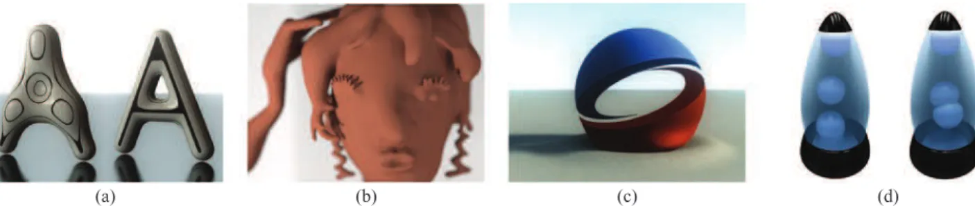
(1) Bulging problem. Implicit blending creates unwanted bulging. For instance, a shape generated by blending together some implicit cylinders defined in the same plane will necessarily be thicker where the cylinders join, as shown in Figure 1(a-left) where the “A” is composed of three blended cylinders. The expected result is the “A” on the right.
(2) Locality problem. Implicit models typically blend at a distance. This is a major problem in modeling applications, where pre-venting the blend between at least some parts of the mod-els (e.g., between the hand and the head of the character in Figure 1(b)) is necessary. The issue is serious in animation too, where pieces of soft material should be allowed to deform each other and eventually blend, but only where they collide.
(d) (c)
(b) (a)
Fig. 1. (a) The unwanted bulge created by standard blending (left) is suppressed by our gradient-based method while preserving the desired topological genus (right). (b) We also prevent small details from blowing up and primitives from blending where they do not intersect. (c) Our generic framework allows the modeling of a wide range of composition operators such as “bulge in contact” and (d) blending (left) and “bulge in contact” (right) combined in the same animation to mimic a lavalamp.
(c) (b)
(a)
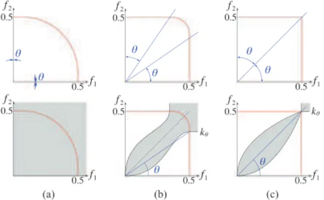
Fig. 2. Three compositions applied to a pair of cylindrical implicit primi-tives forming a cross: (a) standard union based on max; (b) clean union; (c) Barthe’s blending operator parameterized by an opening angle θ . First row: plots of g(f1, f2) where the axes are f1 and f2. Black lines:
some iso-curves, white line: 0.5-iso-curve (surface of interest), background color: gradient direction with vertical (respectively, horizontal) gradient in blue (respectively, in red), green lines: boundaries outside of which g = max(f1, f2). Second row: implicit surface g(f1, f2) = 0.5. Some
iso-lines of g are depicted in a horizontal cutting plane.
(3) Absorption problem. Sharp and thin details are smoothed and they blow up when blended into larger implicit primitives, since they are totally included into the support region of the latter. This problem prevents the creation of thin details such as the eyelashes in Figure 1(b). This is why implicit surfaces have the reputation of only producing simple, blobby shapes.
(4) Topology problem. Lastly, although implicit modeling is an excellent way of generating arbitrary topologies, blending often produces material that will fill a hole that a designer intended, for example, the center of the “A” in Figure 1(a-left). The user has no easy way to control, or at least to predict, the resulting topology.
Solving the preceding problems is essential for both construc-tive modeling and animation. While individual solutions have been proposed, none of them solves all these four issues at once. Doing so efficiently opens the way to many applications, from sketch-based interactive design of 3D shapes (Figure 1(b)) to the inter-active animation of deformable solids (Figures 1(c) and 1(d)). We
review the state-of-the-art and the contributions before presenting the required technical background and our general solution to these four problems.
1.1 Previous Work
Implicit surfaces are well known for their ability to combine shapes by simply composing the associated field functions. Composition is generally expressed as a binary operation, except for the n-ary operators; max, which results in a union and sum, which generates smooth blending between the input shapes [Sabin 1968; Ricci 1973; Blinn 1982]. Improving composition operators has been a major topic of research, and modeling techniques were enhanced by the introduction of clean union operators generating an exact union of the input shapes but with a smooth field everywhere else and of blending operators with local shape control [Pasko et al. 1995; Barthe et al. 2004]. Other operators were developed for animation applications, such as the generation of a contact surface surrounded by bulges when soft objects collide [Cani 1993].
The elimination of the bulging problem was only tackled in two seminal papers: Rockwood [1989] proposed an operator, the su-perelliptic blend, where the range of the blend is parameterized by the cosine of the angle between the field gradients. With this formulation, the blend smoothly transitions to a union where the composed objects’ surfaces become collinear. Even though sup-pressing the unwanted bulges, this operator was C0 only and
in-creased both the locality problem and the topology problem, as reported in Bloomenthal [1997a]. The latter discussed alternative solutions for the n-ary composition of skeleton-based primitives: the kernels or the skeletons of convolution surfaces were used to parameterize a switch from sum to max operators. In addition to not being generally applicable, the lack of smoothness of these early solutions limited their usability in the case of successive blends. Our work builds on Rockwood [1989] since our new composition operators are smooth functions of the angle between field gradients. Although identified early [Bloomenthal 1997b], the locality prob-lemwas only solved recently in a general setting [Pasko et al. 2005; Bernhardt et al. 2010]. The proposed solutions are based on an extra implicit primitive, the blending volume, whose field is used to interpolate between blending and clean union (such as those of Figure 2). Bernhardt et al. [2010] automatically generate blending volumes around intersection curves and sets parameters such that small primitives do not blow up, providing a solution to the absorp-tion problemas well, however, this method has some drawbacks. (1) Only G1 continuous field functions are produced leading to
(a) (b) (c) Fig. 3. Bernhardt’s operator interpolating between clean union and Barthe’s blending. The distortions of the iso-curves of g (a) result in a G1-only implicit surface (b) which still has a bulge on top and exhibits a poor curvature distribution, shown by depicting reflection lines (c).
(2) Computations involve sampling the intersection curve be-tween the two input surfaces or extracting the curve from the intersection of the meshes used for display. This makes the so-lution costly and not scalable, especially in applications where many intersection curves would need to be generated at differ-ent resolutions, such as in a detailed model.
The new method presented here is a more general, scalable ap-proach and is able to restrict blending to regions where the input shapes intersect. At the same time the topological genus of the re-sulting shape can be constrained to remain that of the union (topol-ogy problem), which none of the previous solutions could achieve. Among recent uses of implicit surfaces, we can notice several experimental sketch-based modeling systems [Savchenko et al. 1995; Karpenko et al. 2002; Alexe et al. 2005; Wyvill et al. 2005; Bernhardt et al. 2008; Brazil et al. 2010] for which our new composition method would be especially useful.
1.2 Contributions
We present a generic family of composition operators that brings a unified solution to the four major problems mentioned before. The key idea is to parametrize the blending by the angle between the gradients of the combined field functions, as suggested by Rockwood [1989]. This enables us to interpolate between a union and a blend in the same composition. Using these operators we generate smooth blending between some parts of input shapes and union elsewhere. Blends near intersections are localized without requiring any extra implicit primitive, which makes the method efficient and scalable. In contrast with early work the operators described using our system are C∞continuous, which is a sufficient
property to handle successive compositions.
Our blending technique preserves sharp details and gives enough control on the blend localization so that in general, the topology of the composed object can remain that of the union, which makes composition predictable and well suited to constructive modeling frameworks. Our operators can also be tuned to animate progressive separation of soft material while preventing disjoint parts from blending at a distance. They can also generate contact surfaces surrounded by bulges, possibly followed by progressive merging, when soft objects collide.
The method is generic among functionally based implicit sur-faces. Although it can be applied to discrete fields as well, where f is defined as some interpolation of sample values stored in a grid, we do not address level-set modeling frameworks since the composed field functions we output are not governed by differential equations. This article derives our solution for local implicit primitives, such as soft objects and metaballs. As explained in the next section, these surfaces are the most challenging to handle since the composed field
has to maintain compact support. However, our framework also ap-plies to globally supported primitives, as we illustrate in Section 5.1 with convolution surfaces. Section 2 presents the necessary back-ground and we refer to Bloomenthal [1997b] for a full description of implicit models.
2. BACKGROUND
Implicit surfaces. A functionally based implicit surface S is the C-iso-surface of a field function f : R3
→ R, defined as S = {p ∈ R3
| f (p) = C}. (1) We can identify two types of field functions: globally supported and locally supported field functions.
In fields of global support, implicit surfaces are defined as 0-iso-surfaces and the inside of the surface can be either defined by points pin space such that f (p) < 0 as in Hoffman and Hopcroft [1985] and Barthe et al. [2001] works, or by points p in space such that f(p) > 0 as in Pasko et al. [1995] works.
Local support field functions are commonly positive, decreasing functions of the distance, for instance, to a skeleton, that vanish at a distance R from this skeleton. A skeleton can be a point, a line segment, etc. In this case, the implicit surface is an iso-surface “around” the skeleton, for example, a sphere if the skeleton is a point. The implicit surface is the 0.5-iso-surface, and we use the convention that f (p) > 0.5 defines the interior and f decreases outside an object.
Composing field functions.One of the strengths of implicit mod-eling is the ability to combine fields to form a new shape, using a composition operator as
f = g(f1, f2), (2)
where g : R2
→ R is a binary composition operator, f1and f2are
field functions defining the combined implicit surfaces, and f is the field function defining the resulting object. As we will see, different operators are to be developed for global and local field functions.
Blending.A standard operator for generating smooth blends is the sum [Blinn 1982]
g(f1, f2) = f1+ f2. (3)
Unfortunately, it does not provide any control on the shape of the resulting blend, and can only be applied to local support field func-tions or to convolution surfaces. Therefore, several binary blending operators were proposed over the years for field functions with global support [Bloomenthal 1997b]. The idea is to blend 0-iso-surfaces while meeting specific limit properties, continuity con-straints, or aspect of iso-curves [Hoffmann and Hopcroft 1985; Rockwood 1989; Barthe et al. 2001]. For instance, the superelliptic blend [Rockwood 1989] is defined as
g(f1, f2) = 1 −· 1 − f 1 r1 ¸t + −· 1 − f2 r2 ¸t + , (4) where [∗]+= max(0, ∗), t controls the shape of the blend, making
it closer to the combined objects when it increases, and r1and r2
control the boundaries of the blend on each combined primitive. This operator exhibits some gradient discontinuities that can be avoided by using the Pasko et al. blending set-theoretic operator [1995] defined as: g(f1, f2) = f1+ f2− q f2 1 + f22+ a0 1 +¡f1 a1 ¢2 +¡f2 a2 ¢2, (5) where a0, a1, and a2have an equivalent effect on the blend than,
re-spectively, t, r1, and r2in Eq. (4). Better field variations and user
defined as
g(f1, f2) = min(f1, f2) − H (|f1− f2|) , (6)
where H : R → R is a piecewise cubic polynomial defining the shape of the blend from user-selected control points.
Union. Another well-known operator performs a union using the max function [Sabin 1968; Ricci 1973]
g(f1, f2) = max(f1, f2). (7)
This operator generates C0 continuous field functions that can
cause creases on subsequent blends with additional surfaces.
Clean union. Clean union operators have been introduced by Pasko et al. [1995] (Eq. (8)) and improved by Barthe et al. [2003] for field functions with global support.
g(f1, f2) = f1+ f2−
q f2
1 + f22 (8)
They improve on the standard max operator whose sharp field is illustrated in Figure 2(a-bottom) by performing a union of the surfaces while providing a smooth field function everywhere else (Figure 2(b-bottom)). In a sense, a clean union operator is a union operator on the combined surfaces and a blending operator of their field functions everywhere else. This allows an object built using such an operator to be later blended with another implicit primitive without introducing unwanted sharp edges into the blend [Pasko and Adzhiev 2004].
Visual representation of binary operators. In their work, Hoffman and Hopcroft [1985] introduce an R2space in which
op-erators g are defined and plotted with the value of the field functions f1and f2respectively as abscissa and ordinate. In this space,
ver-tical lines represent the iso-surfaces of the field function f1 and
the horizontal lines, those of the field function f2. The top row of
Figure 2 illustrates three operators plotted in this space in which the white line represents the object iso-surface. The composition oper-ator g = max is represented as in Figure 2(a) while a clean union operator is represented as in Figure 2(b) and a blending operator that smoothly links iso-surfaces of the field function f1with those
of the field function f2at the vicinity of their intersection (i.e., close
to f1= f2) is represented as in Figure 2(c).
Composing locally supported field functions. When using locally supported field functions, primitives are defined by 0.5-iso-surfaces and field functions uniformly equal zero outside the boundary of their support. Thus, composition operators have to be such that g(0, f2) = f2(on and outside the support of f1, g
repro-duces the field function f2) and g(f1,0) = f1(on and outside the
support of f2, g reproduces the field function f1). This also implies
that g(0, 0) = 0. These properties make the definition of composi-tion operators more subtle and tedious than for global supports. All these properties are fulfilled by the operators presented in Figure 2. For instance, the clean union operator presented in Barthe et al. [2004], similar to the one depicted in Figure 2(b), is defined as g(f1, f2) = max(f1, f2) if µ f1≤ 12and µ f2≥ q f1 2 or f2≤ 2f 2 1 ¶¶ or µ f1> 12and µ f2≤ q f1 2 or f2≥ 2f 2 1 ¶¶ {C : ˆhC(f1, f2) = 1} otherwise (9) in which ˆhCis defined as ˆhC(f1, f2) = q (f1−2C2)2+(f2−2C2))2 C−2C2 if f1≤ 12 r ³ f1−√C2 ´2 +³f2−√C2) ´2 C−√C2 otherwise. (10)
An intricate closed-form solution for the computation of C is given in Barthe et al. [2004]. For blending operators, the sharpness of the blending shape can be controlled by a parameter t if the sum is replaced by [Ricci 1973]
g(f1, f2) =¡f1t+ f t 2
¢1t . (11)
However, if some additional control is required on the blend boundary, as was achieved in the global support case through Eqs. (4), (5), and (6), then the blending operator proposed in Barthe et al. [2004] needs to be used. This operator is illustrated in Figure 2(c) with θ = θ1= π2 − θ2and defined as
g(f1, f2) =
max(f1, f2) if f2≤ tan(θ1)f1or f1≤ cot(θ2)f2
{C : ˜hC(f1, f2) = 1} otherwise
(12) in which f2= tan(θ1)f1and f1= cot(θ2)f2correspond to the green
lines in Figure 2(c) (the max is used under the first line and on the left of the second). In between these two lines, ˜hCis defined as
˜hC(f1, f2) = (f1− C. cot(θ2))2 (C − C. cot(θ2))2 +(f2− C. tan(θ1)) 2 (C − C. tan(θ1))2 (13) and θ1, θ2control the boundaries of the blend on each combined
primitive (as r1, r2in Eq. (4) and a1, a2in Eq. (5)).
Opening angles to control the blend. Our solution is based on the work by Barthe et al. [2004] we already mentioned, in which the operator g, is designed to:
(1) give fine control over the resulting shape, as does the superellip-tic blend [Hoffmann and Hopcroft 1985; Hsu and Lee 2003]; (2) avoid the gradient discontinuities in the field function exhibited
by displacement blends [Rockwood 1989]; (3) handle field functions with local support.
The solution presented in Eq. (12) uses the concept of an opening angle θ ∈ [0, π/4] (Figure 2(c)) first introduced in Barthe et al. [2003]. The blend is delimited by boundary lines (green lines in Figure 2(c)). Inside these boundaries the iso-lines of g(f1, f2) are
arcs of ellipses defined in Eq. (13) (as suggested in Hoffmann and Hopcroft [1985]). Outside, no blend occurs and the resulting field function is defined as f = g(f1, f2) = max(f1, f2) (Eq. (12))
in order to exactly reproduce one of the fields of the input field functions. The boundary lines are controlled by varying the opening angle θ so that any intermediate blending (illustrated with θ = π/8 in Figure 2(c)) can be produced between a full blend when θ = 0 and a union (g = max) when θ = π/4 (Figure 2(a)). When θ ∈ [0, π/4], this operator is G1
continuous and when θ = π/4, it is C0.
In practice, the opening angle can be set automatically from a point p, selected in object space R3, on one of the primitives
where the user wants to switch between blending and union. For instance, suppose that the point p(x, y, z) is selected on the 0.5-iso-surface of the field function f1, that is, f1(p) = 0.5. Then, in
the R2 space (Figure 2(c) top) the opening angle θ is calculated
) e ( ) d ( ) c ( ) b ( ) a (
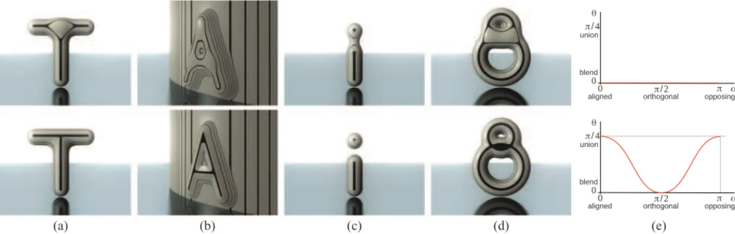
Fig. 4. Comparison between standard blending (first row)—equivalent to a null opening function—and our method (second row) with a opening function that smoothly switches from clean union when α = 0 or α = π to blending when α = π/2. Our solutions to: (a) unwanted bulge; (b) blow up of small details; (c) blending at distance; (d) topology modification; (e) plot of θ (α).
as θ = arctan(f2(p)/f1(p)) = arctan(2f2(p)). The point p can
also be set automatically from the relative size of the composed primitives [Bernhardt et al. 2010].
Interpolating between clean union and blending. Opera-tors interpolating between clean union and blending are able to perform both union and a smooth blend in the same composition. For instance, they enable the combined objects to blend where they are in contact while avoiding any shape deformation everywhere else. They have been introduced by Pasko et al. [2005] for globally supported field functions. Pasko’s operator is defined by Eq. (5) in which the coefficient a0varies: if a0 = 0, the operator performs a
clean union (as in Eq. (8)), and the larger a0, the larger the blending.
Bernardt et al. [2010] proposed such an operator for locally sup-ported field functions. This operator linearly interpolates between the clean union operator defined in Eq. (9) and the blending opera-tor defined in Eq. (12). The limitations of these methods have been discussed in Section 1.1 and Bernhardt’s operator is illustrated in Figure 3. Note that the clean union operator introduced in Barthe et al. [2004] (Figure 2(b)) does not support the insertion of an open-ing angle that would allow the interpolation between a blend and a clean union.
3. GRADIENT-BASED COMPOSITION
Let f1and f2be the field functions of the implicit primitives to be
composed and g be the composition operator we are looking for. As in Rockwood [1989], we claim that g should not only depend on f1and f2, but also on their gradients. Indeed, this appears as a
pertinent option to smoothly blend intersecting shapes where they form a sharp angle, while avoiding bulges where their surfaces are already aligned. This section first presents the key features of our solution. We then explain the field continuity issues that motivate the introduction of a family of quasi-C∞operators in Section 4.
3.1 Controlling Opening from Angle between Gradients
As we just mentioned, g should be able to generate smooth blending between selected parts of the input shapes and union elsewhere. Following Barthe et al. [2004] we choose g with an opening angle parameter θ ∈ [0, π/4] (see Figure 2(c) and Section 2). θ controls
the locality of the blend, that is, the limit values in the (f1, f2) space
out of which a union is computed.
The key feature of gradient-based blending is to define the open-ing angle θ as a function of the angle α between the field gradients at the query point p
θ = θ(α(p)) with α(p) = arccos ∇f1(p) · ∇f2(p) k∇f1(p)kk∇f2(p)k
, (14) where α is the angle between the field gradients and the opening angle θ : [0, π ] → [0, π/4] is defined as a continuous function we call an opening function.
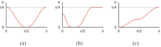
While a constant opening function θ applies the same type of composition everywhere along the input surfaces (such as smooth blending, shown in the first row of Figure 4), choosing opening functions that adequately tune the opening angle according to α allows us to seamlessly solve the four challenging problems we mentioned. Figure 4 shows how this is achieved; from left to right we have:
(a) the bulging problem: The “T” in the top row shows the inflation produced by smooth blending where surfaces are aligned (α close to 0). To avoid this, the opening function should switch to union when α = 0 (aligned gradients). This is done by choosing θ such that θ (0) = π/4 (union for aligned gradients) and θ(π/2) = 0 (blending for orthogonal gradients).
(b) This behavior also naturally prevents the absorption problem on small details since the inflation produced by the blend is gradually reduced as we come close to the “top” of sharp features (where the input surfaces are aligned).
(c) The locality problem occurs when two surfaces come close to each other and blend while they do not intersect, so when α is close to π. This is easily avoided by choosing θ such as θ (π ) = π/4 (union for opposing gradients) and θ (π/2) = 0 (blending for orthogonal gradients).
(d) This setting also avoids the topology problem, that is, the change of topological genus shown on top, since there are points inside each handle where the angle between gradients is π and which will therefore remain outside of the composed shape.
The opening functions used to generate these compositions are depicted in Figure 4(e). Note that the one on the second row, which
(a) (b) (c)
Fig. 5. (a) Two cylindrical implicit primitives are combined using Barthe’s G1operator, where our gradient-based opening function is used to set the
opening angle. The resulting shape still looks smooth; (b) a third primitive is added with the same blending operator. A C0sharp crease now appears;
(c) same scene using our new quasi-C∞blending operator.
we call the camel opening function for its shape, solves all four challenging problems we mentioned. It will be fully described in Section 5.
3.2 Continuity Issues
Computing composition based on the gradients of the input fields having a finite level of continuity locally causes a loss of one order of continuity for the resulting field. This decrease cannot be avoided, but efforts can be made such that neither the opening function θ nor the composition operator g (based on it) introduce any extra source of discontinuity, which could cause artifacts in case of consecutive blends. In particular, Barthe’s operator [Barthe et al. 2004], depicted in Figure 2(c), cannot be used in our framework since it is G1only
and sets up a transition to a standard, C0-only union. If the opening
angle of this operator is set to a function θ of the field gradients, it generates a G1field function with the expected blend after the first
composition (Figure 5(a)) and the loss of continuity after each com-position results in a C0field function with a sharp edge in the second
blend (Figure 5(b)) while a smooth blend as the one illustrated in (Figure 5(c)) was expected. Higher-degree polynomials could be used to define the composition operator, but this would still limit the number of compositions that can be consecutively performed in the same region. Instead, our goal is to define C∞operators g based
on C∞opening functions θ and to set them to control transition to
a clean union (with a smooth field everywhere outside the surface of interest) when θ = π/4.
The constraint for g and θ to be C∞is in fact theoretical: in
prac-tice, we just need g and θ to approximate some C∞functions at a
given precision. This has to be done without introducing oscillations in the field, since the latter would result in curvature artifacts. We say that a function verifying this looser constraint is quasi-C∞
con-tinuous. Relaxing our continuity constraint to quasi-C∞will enable
us to efficiently store our operators as textures on the GPU and to evaluate them with hardware linear interpolation.
Section 4 introduces our opening functions and our new compo-sition operators, which are applied to shape modeling and animation in Section 5. In these sections, the input fields are supposed to be singularity free, that is, with smoothly varying, nonzero gradients vectors. The application of our framework to more general settings will be discussed in Section 6.
4. QUASI-C∞OPERATORS
4.1 Opening Functions
(a) (b) (c)
Fig. 6. Role of the slope of θ in blending. The red (respectively, blue) vectors are gradients of the horizontal (respectively, vertical) primitive. (a) Union; (b) blending with a sharp opening function (w0 = w1 = 3):
unwanted bumps appear where the surfaces are almost aligned, since θ falls very quickly to 0 there; (c) tuning the slope of θ according to the type of input primitives while keeping its other parameters unchanged solves the problem. Here, we set w0= w1= 1, a value preselected for soft objects.
Q1 Q2 Q0 A0 A1 A2 P 0 P/4 A0=0 A1=P/2 A2=P Q ) b ( ) a (
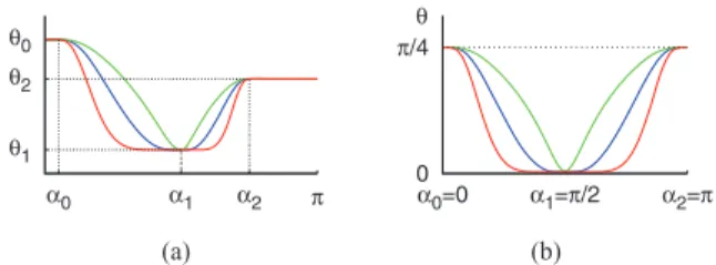
Fig. 7. (a) The 8 parameters of a opening function θ with w0 = w1
respectively equal to 3, 1, and 1/3 for the red, blue, and green curves; (b) three possible opening functions for the blend in Figure 6, using the same values for w0and w1.
into the opening angle of the composition operator. Based on the work of Section 3 this family of functions should be flexible enough to implement various modes of conversion, including, but not re-stricted to those of Figure 4(e). Opening functions designed to model organic shapes and to animate contact situations will be shown in Section 5. The family of functions needed for θ should enable to set some key values and provide some slope control, without which unwanted bumps may appear, depending on the slopes of the input fields around regions where a clean union is applied. See Figure 6. We therefore use a class of functions θ (α), α ∈ [0, π] defined from eight parameters α0, α1, α2, θ0, θ1, θ2, w0and w1. We have
θ(α) = θ0 α ≤ α0 ³ κ³α−α1 α0−α1 ´´w0 (θ0− θ1) + θ1 if α ∈]α0, α1] ³ κ ³ α−α1 α2−α1 ´´w1 (θ2− θ1) + θ1 if α ∈]α1, α2[ θ2 otherwise (15) where κ(x) = 1 − exp à 1 − 1 1 − exp¡1 − 1 x ¢ ! . (16) This function is controlled with eight parameters: three values of αi(i = 0, 1, 2), where α0and α2are limits of the intervals [0, α0]
and [α2, π] in which θ is set to be constant, and the three associated
values for θ (θ0= θ(α0), θ1= θ(α1), θ2= θ(α2)) and two additional
parameters w0and w1controlling the slope of the opening function
in respectively [α0, α1] and [α1, α2]. See Figure 7. In order to ensure
C∞continuity, θ is piecewise defined from a function κ of class C∞
that is flat at the boundaries of its support (i.e., all their successive derivatives equal zero).
In this section we describe a practical set of C∞ functions for
(a) (b) (c)
Fig. 8. Our operator g. First row: The opening angle θ defines the width of the region where composition (here, smooth blend) is applied, at the level of the iso-value (red iso-curve). Second row: The boundary curves kθbound
the region where the values of g are computed with ¯g (light grey area). A max operator is used outside. (a) Opened operator (θ = 0); (b) intermediate situation; (c) closed operator (θ = π/4).
4.2 Composition Operators
Let us now define another family of quasi-C∞functions for the
com-position operator g. This operator should produce smooth blends and also be able to generate other useful compositions, such as bulges when soft objects come in contact [Cani 1993]. Whatever the type of composition, the operator should be parameterized by the opening angle θ, θ ∈ [0, π/4]. The challenge is to define an operator that will fully apply the composition when θ = 0 (opened operator, e.g., a smooth blend), and gradually switch to a clean union between the input shapes when θ = π
4 (closed operator),
while avoiding the limitations of Bernard’s operator (Section 1.1 and Figure 3).
Following the construction of operators with an opening angle, our operator g uses the angle θ to define the width of the region where the composition is applied at the level of the iso-value (red iso-curve in Figure 8). We also use boundary curves kθ bounding
the region where the values of g modify the field of the combined field functions f1and f2(light grey area in Figure 8). In this region,
g = ¯g and g = max outside. A critical contribution here is the spe-cial shape of our boundary curves kθwhen θ varies from 0 to π/4
(Figure 8(b)). This shape has been specifically designed to continu-ously interpolate between the vertical and horizontal boundary lines of a standard blend (θ = 0, Figure 8(a)) and the smooth boundary curves intersecting at f1 = f2 = 0.5 of a clean union (θ = π/4,
Figure 8(c)).
We introduce a family of C∞boundary curves whose intermediate
shape is shown in the second row of Figure 8(b) and in Figure 9(c). These boundary curves are defined by C∞functions kθ(f ), where
f is either f1or f2. We set kθ(f ) = tan(θ)/2 inside of the implicit
primitives, where f ≥ 0.5. Outside the primitives, where f < 0.5 the expression of kθis kθ(f ) = tan(θ ) 2 µ 4 1 + tan(θ)λθ(f ) ¶2 , (17) with λθ(f ) = ( f if f ≤tan(θ ) 2 1−tan(θ) 4 φ(22f −tan(θ)1−tan(θ)) + tan(θ ) 2 otherwise (18)
and φ is a function ensuring the C∞continuity of λ
θ. φ is computed
by binary search at the required precision, from φ−1defined as:
φ−1(x) = x +1 elog µ log µ 1 ν(x)+ 1 ¶ + 1 ¶ , (19) where e = exp(1) and with
ν(x) = exp (exp(e − ex) − 1) − 1. (20) In practice, the computation of φ does not affect efficiency since our operators are precomputed on the GPU (see Section 4.3). The value of g inside the region bounded by the boundary curves kθ(in
grey on Figures 8 and 9(c)) is defined by an operator ¯g : R2
→ R, which sets the type of composition we desire. The equation of our composition operator g is thus
g(f1, f2) =
½ max(f1, f2) if f1≤ kθ(f2) or f2≤ kθ(f1)
¯g(f1, f2) otherwise .
(21) The function ¯g is defined from a silhouette curve ¯s(ϕ) : [0, π/2] → R describing the shape of the iso-curves of ¯g as il-lustrated in Figure 9. For instance, an arc-of-a-circle is created using ¯s(ϕ) = 1, ∀ϕ. For given values of f1and f2, the value of our
operator ¯g(f1, f2) is computed by solving the following equation in
C: ¯g(f1, f2) = {C : ¯hC(f1, f2) = 1} (22) with ¯hC(f1, f2) = p (f1− kθ(C))2+ (f2− kθ(C))2 ¯s(ϕ) (C − kθ(C)) , (23) and ϕ = arctanf2− kθ(C) f1− kθ(C) , (24) which expresses the fact that the iso-curves of ¯g are scaled versions of ¯s. In practice, Eq. (23)) does not always have a closed-form solution. We thus precompute sampled values of g and interpolate them on the GPU, as detailed in Section 4.3.
Using any C∞silhouette curve ¯s, such that ¯s(0) = ¯s(π/4) = 1
and with flat derivatives at the level of the boundary curve (so that g’s derivatives match those of the max function) is thus sufficient for getting a C∞operator g. To illustrate how different these silhouette
curves can be and the variety of resulting compositions, Section 5 will give the equations of the curves we use for smooth blending and for a “bulge-in-contact” composition.
4.3 Implementation on the GPU
As discussed earlier, we use families of opening functions and of composition operators that have all the required smoothness properties, but that may not have any closed-form expression. For efficiency, we developed a GPU implementation for these functions, which enables us to apply gradient-based compositions in real time. The GPU implementation is based on the following precomputa-tions: the opening function which gives θ from the angle between gradients (Eq. (15)) and its derivative ∂θ
∂αare stored as 1D textures.
We also precompute values of the operator g and of its partial derivatives ∂g
∂f1,
∂g ∂f2,
∂g
∂θas functions of θ , f1, and f2in a regular grid
stored as a 3D texture. This is done efficiently using the following procedure: The values of g are computed by grid slice (fi
1, f j 2),
(i, j ) ∈ [0; N − 1]2, for each grid coordinate θ
k, k ∈ [0; N − 1] (N3
being the size of the grid). In a slice, for each i, we set Ci= f1iand
we follow the Ci-iso-curve Giof g and update the sample values as
(a) (b) (c)
Fig. 9. (a) A silhouette curve ¯s(ϕ); (b) defines the shape of the C-iso-curves of ¯g to produce (c) the corresponding operator g.
(a) (b)
Fig. 10. Computation of the interpolation parameter γ1(a) (respectively
γ2(b)), defined as the distances from X to Gi(respectively from X to Gi+1),
used to compute ¯g at a sample point X in Eqs. (25), (26), and (27).
—Outside of the boundary curves, that is, for each j such that f2j<
kθ(f1i), g = max(f1, f2) (Eq. (21)), so we set g(f1i, f j 2) = Ci
and g(f2j, f1i) = Ci.
—Inside of the boundary curves, for each sampling point X(Xx, Xy)
located in the bounding box of the silhouette curve ¯s scaled by (Ci+1− kθ(Ci)) with the bottom-left corner in Oi, we compute
γ1and γ2as in Eqs. (26) and (27). When γ1 ≥ 0 and γ2 ≥ 0,
X is between Giand Gi+1, that is, the Ci-iso-curve and the Ci+1
-iso-curve, and we compute ¯g(X) by linearly interpolating Ciand
Ci+1as in Eq. (25). We have
¯g(X) = γ2Ci+ γ1Ci+1 γ1+ γ2
(25) with
γ1 = kX − Oik − ¯s(ϕi) (Ci− kθ(Ci)) (26)
γ2 = ¯s(ϕi+1) (Ci+1− kθ(Ci+1)) − kX − Oi+1k (27)
where
Oi= (kθ(Ci), kθ(Ci)) and ϕi= arctan
Xy− kθ(Ci)
Xx− kθ(Ci)
. (28) Once all the values of g are computed, its partial derivatives are evaluated using finite differences and stored in other grids.
During field queries for a composed implicit surface, the values in these textures are linearly interpolated on the GPU: we first get θfrom the gradients of the input fields and then g(f1, f2) with this
specific opening angle θ . Depending on the primitive, gradients are either computed using a closed-form expression or finite differ-ences. To efficiently apply successive compositions, the gradient of
163 323 643 1283 max error 5 .03× 10 −2 2 .90× 10 −2 1 .39× 10 −2 6 .72× 10 −3 mean error 2 .97× 10 −3 1 .43× 10 −3 7 .32× 10 −4 3 .69× 10 −4
Fig. 11. Close-up on the surface obtained after three successive blends when g is stored into textures of different resolutions. The piecewise linear interpolation generates artifacts in reflections (here illustrating the continuity of the fifth derivatives) with the 163and 323grids that are not perceptible
using higher resolutions. The third and fourth rows respectively give the max and mean approximation error provided by the trilinear interpolation of the precomputed values.
g(f1, f2) is computed as ∇g = ∇f1 ∂g ∂f1 + ∇f 2 ∂g ∂f2+ ∇α ∂θ ∂α ∂g ∂θ. (29) A consequence of our GPU implementation is that the operators we use in practice are not exactly the C∞functions we developed, but
quasi-C∞approximations of the latter: indeed, linear interpolation
of values in a texture prevents unwanted oscillation and enables us to approximate the functions at any desired precision. We tested the method with 163, 323, 643, and 1283grids for g and its gradients.
Figure 11 shows the improvement of reflection lines on a very close view of a composed primitive when texture resolution increases. Our current implementation uses 1283grids which is accurate enough
to prevent any visual artifact, even after multiple compositions. Note that if a very high precision was required, for example, for a manufacturing application, an offline evaluation mechanism with bounded error could be set up, where binary search would be used to find the resolution needed to obtain a given error bound.
5. APPLICATIONS
In this section, we present applications of our generic composition operators to constructive modeling and animation. This leads us to define specific silhouette curves ¯s and the associated opening functions θ .
5.1 Smooth Blending for Constructive Modeling
Being able to smoothly blend arbitrary shapes is one of the most useful compositions in constructive modeling systems. To create a
0 1 0 1 sb -(c) (b) (a)
Fig. 12. Close view of the top of the cross formed by two blended cylin-drical primitives: (a) using Bernhardt’s blending; (b) using our operator gb
with a opening function preventing the unwanted bulge; (c) plot of ¯sbfrom
which gbis derived.
(a) (b) (c)
Fig. 13. Plots of gbin the (f1, f2) space for different values of the opening
angle θ . (a) Opened operator: θ = 0. (b) θ =π
8. Note the improved shape of
the iso-curves compared to those of Figure 3; (c) closed operator, resulting in a clean union: θ =π
4.
good blending operator ¯gb, we need a C∞silhouette curve ¯sb, which,
in addition to meeting the value and derivative constraints listed at the end of Section 4.2 (values 0.5 and null derivatives of every order at the extremities), avoids curvature oscillations as much as possible, as illustrated in Figure 12.
Our solution plotted in Figure 12(c) is a symmetric silhouette curve whose curvature monotonically increases, with a maximum at ϕ = π/4, then decreases back to zero. We define ¯sbas
¯ sb(ϕ) = 1 − 1 elog µ log µ 1 ν(ϕ)+ 1 ¶ + 1 ¶ , (30) where ν is defined in Eq. (20).
For our precomputations of g on the GPU, we express this profile function in polar form, as ¯sb(ϕ), by sampling the curve at points
Xi= (xi,s¯b(xi)) and precomputing the value of ϕiat each Xi. To
evaluate the function ¯sb(ϕ), we use binary search to find the interval
[ϕi; ϕi+1] containing ϕ, and then use linear interpolation. Although
not exactly flat at the boundaries, this silhouette curve has zero derivatives in ϕ = 0 and ϕ = π/2 up to an error of ǫ = 10−5, which
is accurate enough for our needs. This operator is illustrated in R2
space in Figure 13 for different values of θ . Its fairness leads to a clear improvement compared with Bernhart’s blending solution as shown with reflection lines in Figures 12(a) and 12(b).
This blending operator gb computed using ¯sb can be combined
with different opening functions according to the need. Our appli-cations to shape modeling lead us to design two specific examples of opening functions.
The first one, whose parameter values are given in the first row of Table I, is called the camel opening function because of the shape of the associated curve (see its plot in Figure 15(a)). It is symmetric and was especially designed to solve, for Wyvill’s local-support soft objects [Wyvill et al. 1986], all four problems mentioned in the Introduction (Figure 4). In the case of CAGD applications, where two primitives join, this opening function provides smooth, predictable blending behavior while preventing bulges.
Table I. Parameter Values Defining Our Different Opening Functions
α0 α1 α2 θ0 θ1 θ2 w0 w1
Camel 0 π/2 π π/4 0 π/4 1 1 Organic 0 π/3 3π/4 π/6 0 π/4 3 1 Contact 0 π/2 π 0 π/10 π/4 1 0.7
The second one, whose parameter values are given in the sec-ond row of Table I, is called the organic opening function (see its plot in Figure 15(b)). It was developed for an interactive modeling system dedicated to the modeling of organic shapes, using global-support convolution surfaces based on the Cauchy kernel [Tai et al. 2004]. Here, being able to model both smooth and sharp features in the same composition is important: for instance, when blending a character’s nose to the head (Figure 1(b)) or the leg and tail of an animal to its body (Figure 14(right)), the junction has to be smooth at the top but sharp at the bottom. To achieve this, our organic opening function is set to be asymmetric: surfaces smoothly blend where they have nearly orthogonal gradients, while a clean union generating sharp creases is used when gradients tend to be in oppo-site directions (see Figure 14(left)). This enables us to get detailed organic-like models with both smooth parts and sharp creases.
5.2 Bulge in Contact for Soft Objects Animation
To illustrate the variety of compositions we can achieve, we de-signed a “bulge-in-contact” operator gc, inspired by Cani [1993],
which instead of blending primitives that intersect, mimics the ef-fect of two surfaces in contact that bulge as if made from a soft material such as rubber (Figures 16, 1(c) and (d)).
Keeping in mind that the silhouette curve ¯s directly gives the shape of the deformation, Figure 16(a) shows the deformation of f1
on the right and of f2on top. We set ¯s such as to create smoothly
increasing and then decreasing bulges. This is done by using values smaller than 0.5 on the silhouette curve. Figure 16(c) shows the resulting point of contact (no deformation) and the deformation as f1and f2overlap.
Defining these contact silhouette curves is done using the para-metric expression ¯sc(t)(xc(t), yc(t)) with
xc(t) = ½ t if t ≥ 1 1 − K exp¡1 − 1 2−t¢ (t − 1) otherwise yc(t) = ½ 1 − K exp¡1 − 1 t¢ (1 − t) if t ≥ 1 2 − t otherwise (31)
for t ∈ [0, 2], where K ∈ [0, 1] is a parameter that controls the thickness of the bump. The effect of K on the iso-curves of ¯gc
is illustrated in Figure 16(a). The curve ¯scis perfectly flat at the
extremities and is, as desired, only C0continuous at ϕ =π 4 in order
to simulate the fold to be created between the two input surfaces. Again, the polar form ¯sc(θ ) can easily be evaluated using binary
search, as done for ¯sbin Section 5.1.
Finally, a contact opening function, whose parameter values are given in the third row of Table I, is designed so that when used with our bulge-in-contact operator, objects do not deform at a distance but bulge when they intersect, mimicking contact between soft objects, as illustrated in Figure 15(c). The operator gc is illustrated with
K = 0.8 in Figures 1(d) and 16(c).
6. RESULTS AND DISCUSSION
Even though the implementation of the set of functions presented here can be considered complex, its usage is not. The functions can
Barthe’s blending “camel” blending “organic” blending “organic” blending in interactive modeling
Fig. 14. Comparison of Barthe’s blending with our operator gb, used either with the camel or with the organic opening function.
0 P/4 0 P/2 P Q 0 P/4 0 P/2 P Q 0 P/4 0 P/2 P Q (c) (b) (a)
Fig. 15. Three useful opening functions: (a) camel and (b) organic opening functions used with the blending operator gb; (c) contact opening function
used with the bulge-in-contact operator gc.
be used in an interactive modeling framework as any other operator; objects are added to the scene, selected, and the operator is applied to two of them. With most traditional implicit operators the resulting shape is fixed after applying the operator. In contrast our new set of functions provide ways to further modify the shape, by altering the silhouette curve and the opening function in a graphical editor, however, most of the useful opening functions are defined in this article and cover most of the practical cases. New opening functions only need be defined for specialized operations.
The usefulness of our generic composition framework for con-structive modeling and animation applications is illustrated in Figures 17 and 1(d). The model presented in Figure 17 has been built using ten different primitives combined with either our blend-ing operator together with the camel openblend-ing function or with our clean union operator (generating sharp edges). In the case of a blend overlapping a sharp edge, we use the procedure presented in Sec-tion 7 and in Figure 19. The object has been created interactively using the Blob-tree [Wyvill et al. 1999] in several sessions over a period of about eight hours. In the “lava lamp” animation, gcis
used in conjunction with our blending operator to also get some blending when bubbles leave the bottom of the lamp. Other in-teresting animation effects can be easily produced by dynamically modifying the opening function parameters during an animation. For instance, Figure 18 illustrates an animation where primitives do not blend when they are not in contact, but do blend (and thus deform each other) when they separate even though they are not in contact anymore, as in standard blending.
Achieving good-quality results leads us to use more complex equations for composition than in all previous methods. The efficient evaluation of our operators is based on precomputation that only needs to be performed once for each operator and for each opening function, and just requires the memory space of a few textures. This implementation allows us to use arbitrarily complex expressions for gand θ , while answering field queries at the cost of a simple texture fetch. Therefore, when designing a new operator, one can focus on the desired effect rather than on the best properties a closed-form equation could achieve. The precomputation of our operator and its partial derivatives in 1283grids takes 600 ms on a Core I7 950 and
their transfer to the device memory from the host memory takes
0 0.2 0.4 0.6 0.8 1 0 0.2 0.4 0.6 0.8 1 (c) (b) (a)
Fig. 16. (a) Plots of ¯scfor K = 0.25 (red), K = 0.5 (green) and K = 0.75
(blue); (b) the corresponding operator gcwhen θ =π8 and K = 0.8; (c) the
application of our operator gc.
Fig. 17. Constructive modeling examples built using our new operators. In this model, clean union and clean difference operators have been used in conjunction with gradient-based blending operators. Both sharp edges and subsequent gradient-controlled blends have thus been efficiently performed.
3 ms. The 786 million evaluations of g required for the rendering of Figure 11 take less than 270 ms on a NVIDIA GTX 480.
7. LIMITATIONS
First, as we emphasized in Section 4.1, adequate slope for the open-ing function has to be used, dependopen-ing on the slope of the input field functions, for not creating extra artifacts when removing a bulge. In practice, we use the interactive feedback of implicit modeling sys-tems to preset the steepness parameters w0and w1of our opening
functions according to the family of field function used. Typically, we need sharper opening functions to blend soft objects based on smooth polynomial field functions than to compose sharper convo-lution surfaces. Once the steepness parameters are set, we design specific opening functions by adjusting the three input values for (αi, θ(αi)). Providing an automatic tuning of the opening function’s
slope would be a better solution. The method, as currently imple-mented, still requires little user interaction since the manual tuning only needs to be done once for a given family of field functions, for each opening function.
A drawback of our gradient-based operators is that they theoreti-cally require at least the continuity of the gradient directions of the field functions f1 and f2 to be combined. Using our composition
Fig. 18. From left to right, the opening function is modified to create different blending behaviors during an animation.
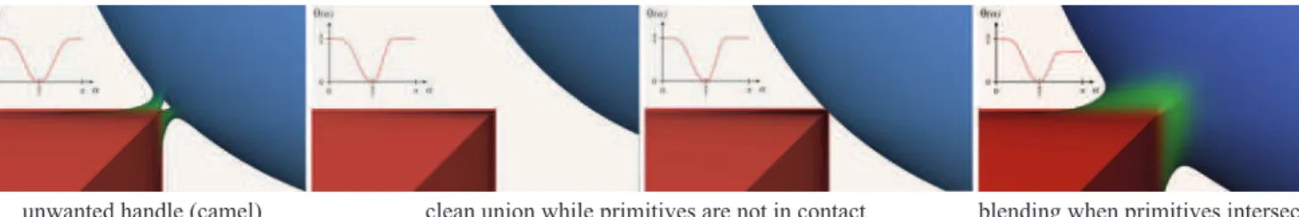
blending when primitives intersect clean union while primitives are not in contact
unwanted handle (camel)
Fig. 19. Composition of a cube and a sphere at a gradient discontinuity (an edge of the cube). On the left, the artifact generated when the camel opening function is used for blending, and then, opening functions solving the problem when the sphere moves and intersects the cube.
framework in a more general setting, where the field may have a few singular points (with null gradients and therefore undefined angle between gradients) would, however, be desirable, as well as using it even for shapes with gradient discontinuities, for example, for primitives with sharp edges. In case of null gradient vectors, we simply decrease the opening angle to min(θ0, θ1, θ2) when the
gradient norm becomes close to null, so that the opening function is constant at the vicinity of the singularity. This only leaves us with the case of artifacts created by discontinuities of the gradient field. This is illustrated by Figure 19(left), where the camel opening function is used for blending in the vicinity of a sharp edge. The problem can be solved in the following way: while primitives are not in contact, an opening function preventing blend is required, and as soon as the primitives intersect, a blend can be progressively performed. This is done easily by manually tuning a few opening function parameters as illustrated in Figure 19. In an animation, the opening function parameters have thus to be preset in key primitive positions such as those presented in Figures 19 and then interpolated during the animation.
As with all recent composition methods, the gradient-based op-erators are restricted to binary compositions of implicit surfaces. This may limit their applicability in situations where many primi-tives need to be symmetrically connected at once. Generalizing the idea of using gradients into n-ary composition operators would be a topic for future work. Similarly, although they can be used to compose convolution primitives, our operators cannot replace the sum performing the convolution integral of each element (points, segment, triangles) of a complex skeleton defining a convolution surface [Bloomenthal 1997b]. We do not provide a solution to the problem of a single convolution primitive unintentionally blending with itself.
8. CONCLUSION AND FUTURE WORK
We have presented a generic family of composition operators appli-cable to both constructive implicit modeling and animation. These operators, implemented in real time on the GPU, allow precise tun-ing of the transition between smooth blends and sharp union within a single composition operation, making compositions both more
general and more predictable. The main feature of our approach is the use of gradient-controlled blending: our operators are not only a function of the field functions to be combined, but also of their gradient. This avoids the well-known weaknesses of implicit mod-eling, such as creating unwanted bulges and blending at distance. In general, the topology of the resulting shape can be set to the topology of the union. Moreover, our operators naturally prevent small details from blowing up even when blended into much larger primitives, thanks to the sharp changes of gradient values. In conse-quence, complex models with both smooth parts and sharp creases can be easily created, in contrast with the common idea that implicit surfaces can only represent smooth, blobby shapes.
The natural extension of using the angle between field gradients would be the use of the information on the norm of these gradients to improve blends. This norm could be used to automatically set the slope parameters of the opening functions, according to steepness of the input fields. Another extension would be to rely on the second derivatives of the input fields to detect fast local gradient variations. This would help us to avoid user interaction currently necessary to adjust opening functions in areas where the field functions are very distorted or at the vicinity of gradient discontinuities such as sharp edges. Lastly, the general methodology we developed for the open-ing functions, that is, definopen-ing C∞curves with some shape control
parameters, could be reused to introduce local-support C∞fields for
implicit primitives. This would ensure always having smooth gra-dient fields, whatever the number of gragra-dient-based compositions.
REFERENCES
ALEXE, A., BARTHE, L., CANI, M.,ANDGAILDRAT, V. 2005. Shape modelling by sketching using convolution surfaces. In Pacific Graphics Short Papers.
BARTHE, L., DODGSON, N. A., SABIN, M. A., WYVILL, B.,ANDGAILDRAT, V.
2003. Two-Dimensional potential fields for advanced implicit modeling operators. Comput. Graph. Forum 22, 1, 23–33.
BARTHE, L., GAILDRAT, V.,ANDCAUBET, R. 2001. Extrusion of 1D implicit
profiles: Theory and first application. Int. J. Shape Model. 7, 179–199.
BARTHE, L., WYVILL, B.,AND DEGROOT, E. 2004. Controllable binary csg
BERNHARDT, A., BARTHE, L., CANI, M.-P.,ANDWYVILL, B. 2010. Implicit
blending revisited. Comput. Graph. Forum 29, 2, 367–376.
BERNHARDT, A., PIHUIT, A., CANI, M. P.,ANDBARTHE, L. 2008. Matisse:
Painting 2D regions for modeling free-form shapes. In Proceedings of
the Eurographics Workshop on Sketch-Based Interfaces and Modeling.
57–64.
BLINN, J. F. 1982. A generalization of algebraic surface drawing. ACM Trans.
Graph. 1,3, 235–256.
BLOOMENTHAL, J. 1997a. Bulge elimination in convolution surfaces.
Com-put. Graph. Forum 16, 31–41.
BLOOMENTHAL, J., ED. 1997b. Introduction to Implicit Surfaces. Morgan
Kaufmann, San Fransisco, CA.
BRAZIL, E., MACEDO, I., SOUSA, M. C.,DEFIGUEIREDO, L.,ANDVELHO,
L. 2010. Sketching variational hermite-rbf implicits. In Proceedings of
the 7t h Sketch-Based Interfaces and Modeling Symposium (SBIM’10).
Eurographics Association, 1–8.
CANI, M.-P. 1993. An implicit formulation for precise contact modeling between flexible solids. In Proceedings of the 20t hAnnual Conference on Computer Graphics and Interactive Techniques (SIGGRAPH’93).313– 320. (Published as Marie-Paule Gascuel).
HOFFMANN, C.ANDHOPCROFT, J. 1985. Automatic surface generation in
computer aided design. Vis. Comput. 1, 2, 92–100.
HSU, P. C.ANDLEE, C. 2003. Field functions for blending range controls on soft objects. Comput. Graph. Forum 22, 3, 233–242.
KARPENKO, O., HUGHES, J.,ANDRASKAR, R. 2002. Free-Form sketching with
variational implicit surfaces. Comput. Graph. Forum 21, 585–594.
PASKO, A.ANDADZHIEV, V. 2004. Function-Based shape modeling:
Math-ematical framework and specialized language. In Automated Deduction
in Geometry, Lecture Notes in Artificial Intelligence, vol. 2930, Springer, 132–160.
PASKO, A., ADZHIEV, V., SOURIN, A.,ANDSAVCHENKO, V. 1995. Function
representation in geometric modeling: Concepts, implementation and ap-plications. Vis. Comput. 11, 8, 429–446.
PASKO, G. I., PASKO, A. A., ANDKUNII, T. L. 2005. Bounded blending for function-based shape modeling. IEEE Comput. Graph. Appl. 25, 2, 36–45.
RICCI, A. 1973. A constructive geometry for computer graphics. Comput. J.
16, 2, 157–160.
ROCKWOOD, A. 1989. The displacement method for implicit blending
sur-faces in solid models. ACM Trans. Graph. 8, 4, 279–297.
SABIN, M.-A. 1968. The use of potential surfaces for numerical geome-try. Tech. rep. VTO/MS/153, British Aerospace Corporation, Weybridge, UK.
SAVCHENKO, V., PASKO, A., OKUNEV, O.,ANDKUNII, T. 1995. Function
representation of solids reconstructed from scattered surface points and contours. Comput. Graph. Forum 14, 181–188.
TAI, C., ZHANG, H.,ANDFONG, J. 2004. Prototype modeling from sketched silhouettes based on convolution surfaces. Comput. Graph. Forum 23, 71–83.
WYVILL, B., FOSTER, K., JEPP, P., SCHMIDT, R., SOUSA, M. C.,ANDJORGE, J. 2005. Sketch based construction and rendering of implicit models. In
Proceedings of the Eurographics Workshop on Computational Aesthetics in Graphics, Visualization and Imaging. 67–74.
WYVILL, B., GUY, A.,ANDGALIN, E. 1999. Extending the csg tree: Warping,
blending and Boolean operations in an implicit surface modeling system.
Comput. Graph. Forum 18,2, 149–158.
WYVILL, G., MCPHEETERS, C.,ANDWYVILL, B. 1986. Data structure for soft