Étude des débits des cours d'eau canadiens dans un climat changeant

ÉTUDE DES DÉBITS DES COURS D'EAU CANADIENS DANS UN

CLIMAT CHANGEANT

MÉMOIRE PRÉSENTÉ

COMME EXIGENCE PARTIELLE

DE LA MAÎTRISE EN SCIENCES DE L'ATMOSPHÈRE

PAR VINCENT POITRAS

UNIVERSITÉ DU QUÉBEC À MONTRÉAL Service des bibliothèques

Avertissement

La diffusion de ce mémoire se fait dans le respect des droits de son auteur, qui a signé le formulaire Autorisation de reproduire et de diffuser un travail de recherche de cycles

supérieurs (SDU-522 - Rév.01-2006). Cette autorisation stipule que «conformément

à

l'article 11 du Règlement no 8 des études de cycles supérieurs, [l'auteur] concède

à

l'Université du Québec

à

Montréal une licence non exclusive d'utilisation et de publication de la totalité ou d'une partie importante de [son] travail de recherche pour des fins pédagogiques et non commerciales. Plus précisément, [l'auteur] autorise l'Université du Québec

à

Montréal

à

reproduire, diffuser, prêter, distribuer ou vendre des copies de [son] travail de recherche

à

des fins non commerciales sur quelque support que ce soit, y compris l'Internet. Cette licence et cette autorisation n'entraînent pas une renonciation de [la] part [de l'auteur]

à

[ses] droits moraux ni

à

[ses] droits de propriété intellectuelle. Sauf ententè contraire, [l'auteur] conserve la liberté de diffuser et de commercialiser ou non ce travail dont [il] possède un exemplaire.))

Je tiens tout d'abord à faire d'incommensurables remerciements à ma directrice de recherche Laxmi Suhama qui m'a donné un soutien indéfectible tout au long de ma maîtrise. J'aimerais également remercier Frank Seglenieks, chercheur à l'Université de Waterloo, qui m'a révélé tous les secrets du schéma de routage W ATroute. J'aimerais aussi remercier Naveed Khaliq, chercheur à Environnement Canada, qui m'a fait bénéficier de son expertise en statistique pour l'analyse d'événements extrêmes. Enfin, j'aimerais saluer les professems et les chercheurs de l'UQAM, ceux d'Ouranos, ainsi que mes collègues étudiants qui sont trop nombreux pour être tous nommés mais dont l'aide et le support m'ont été indispensables.

TABLE DES MATIÈRES

LISTE DES TABLEAUX v

LISTE DES FIGURES vi

LISTE DES ACRONYMES ix

LISTE DES SYMBOLES xi

RÉSUMÉ xiv

INTRODUCTION l

ABSTRACT 9

1. Introduction Il

.2. Model, data and methods 13

2.1. Canadian RCM 13 2.2. Observational data 14 2.3. Methodology 15 2.3.1 Mean flows 16 2.3.2 Extreme flows 19 3. Results · 20 3.1. Mean flows 20 3.1.1. Validation 20 3.1 .2. Projected changes 23 3.2. Low flows 24 3.2.1. Validation 24 3.2.2. Projected changes 26 3.3. High flows 27 3.3.1. Validation 27 3.3.2. Projected changes 28

4. Summary and conclusions 28

TABLEAUX 32

FIGURES 36

RÉFÉRENCES 63

CONCLUSION 69

ANNEXE A: ÉQUATION DE ROUTAGE 74

LISTE DES

TABLEAUX

Tableau Page

Table 1: Lake routing parameters for the Great Lakes. Observed levels in current climate are from NOAA and projected departure levels for future climate follow Angel and Kunkel

(2009) 33

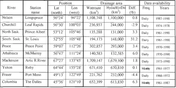
Table 2: Details of the gauging stations used in the validation of streamflows. Data come from HYDAT for ail basins except Yukon and Columbia and are available on a daily basis.

RivDis dataset is used for Yukon and Columbia and are available on a monthly basis 33

Table 3: Comparison of observed and CGCM·ERA40c mean daily hydrographs (monthly for Yukon and Fraser). The comparison period depends on the availability of observed data (see

Table 2) 34

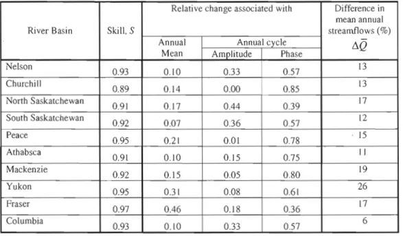
Table 4: Comparison of CGCM·ERA40c and CGCM·CGCMc simulated 30-year mean daily

hydrograph (1961-1990) 34

Table 5: Comparison of CGCM·CGCMc (1961-1990) and CGCM·CGCMf (2041-2070)

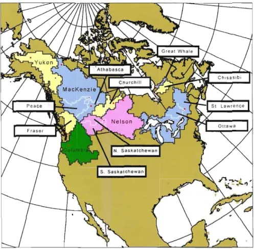
Figure Page Figure 1: CRCM computationa1 domain in polar stereographic projection, with the studied basins. The ones in white are the sub-basins; Ottawa is a subbasin of St. Lawrence, North and

South Saskatchewan that of Nelson and Peace and Athabasca that of MacKenzie 37

Figure 2: Observed (black), CRCM·ERA40c unrouted (purple) and routed (green) mean daily hydrographs. The comparison period varies from basin to basin, depending on the

availability of observational data, and is indicated on each subfigure 38

Figure 3: 30-year mean daily hydrographs for CRCM·ERA40c (1961-1990; green), CRCM·CGCMc (1961-1990; blue) and CRCM·CGCMf(2041-2070; red). The shaded area (for the blue and red curves) represent the member spread of respective ensembles. Data have

been smoothed with a 31-day running mean 39

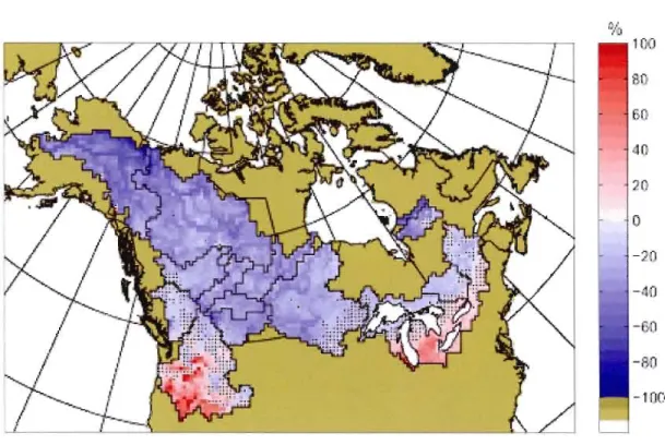
Figure 4: Spatial distribution of the boundary forcing errors associated with the 30-year mean annual streamflows (in %). Dots are used to highlight grid cells where the forcing

errors are not significant according to a {-test at significance level of 0.05 40

Figure 5: Spatial distribution of the boundary forcing errors associated with the 30-year mean winter (DJF) strearnflows (in %). Dots are used to highlight grid cells where the forcing

errors are not significant according to a {-test at significance level of 0.05 .41

Figure 6: Spatial distribution of the boundary forcing errors associated with the 30-year rnean springs (MAM) strearnflows (in %). Dots are used to highlight grid cells where the forcing

errors are not significant according to a {-test at significance level of 0.05 .42

Figure 7: Spatial distribution of the boundary forcing errors associated with the 30-year mean summer (JJA) streamflows (in %). Dots are used to highlight grid ceIls where the forcing

errors are not significant according to a {-test at significance level of 0.05 .43

Figure 8: Spatial distribution of the boundary forcing errors associated with the 30-year mean autumn (SON) streamflows (in %). Dots are used to highlight grid cells where the forcing

Vil

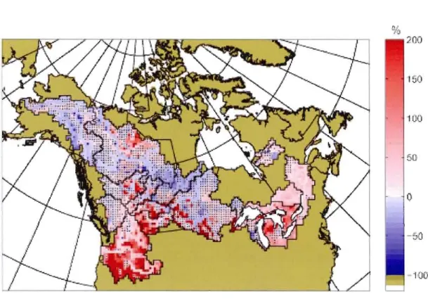
Figure 9: Spatial distribution of the projected changes to the 30-year mean annual

streamflows (in %). Dots are used to highlight grid cells where the projected changes are not

significant according to a (-test at significance level of 0.05 .45

Figure 10: Spatial distribution of the projected changes to the 30-year mean win ter (DJF)

streamflows (in %). Dots are used to highlight grid cells where the projected changes are not

significant according to a (-test at significance level of 0.05 .46

Figure Il: Spatial distribution of the projected changes to the 30-year mean springs (MAM)

streamflows (in %). Dots are used to highlight grid cells where the projected changes are not

significant according to a (-test at significance level of 0.05 .47

Figure 12: Spatial distribution of the projected changes to the 30-year mean summer (JJA)

streamfIows (in %). Dots are used to highlight grid cells where the projected changes are not

significant according to a (-test at significance level of 0.05 .48

Figure 13: Spatial distribution of the projected changes to the 30-year mean auturnn (SON) streamfIows (in %). Dots are used to highlight grid cells where the projected changes are not

significant according to a (-test at significance level of 0.05 .49

Figure 14-a: Scatter plots of annual 15-day 10w flows for observed (black triangles), CRCM·ERA40c (green cicles) and CRCM·CGCMc (blue circles). Also shown are the distribution (in %; solid curves) of the 15-day low flow events that have been smoothed with a 7-day running mean. The left axis corresponds to the scatter plot and the righl axis

corresponds to the distribution 50

Figure 14-b: Same figure 14-a but without observations to allow a better resolution of the

vertical axis 51

Figure 15: Spatial distribution of the boundary forcing errors associated with the IO-year

retum levels of 15-day low flows for the FMAM period (in %) 52

Figure 16: Spatial distIibution of the boundary forcing errors in the 10-year return levels of

15-day low flows for the ASOND period (in %) 53

Figure 17: Scatter plots of annual 15-day low flows for CRCM·CGCMc (blue circles) and CRCM·CGCMf (red cu-cles). Also shown are the distribution (in %; solid curves) of the 15­ day low flow events that have been smoothed with a 7-day running mean. The left axis

corresponds to the scatter plot and the right axis cOITesponds to the distribution 54

Figure 18: Spatial distribution of the projected changes to the lO-year return levels of 15-day

low flows for the FAMM period (in %) 55

Figure 19: Spatial distribution of the projected changes to the 10-year return levels of 15-day

Figure 20: Box plots of the annual number of days with flows below the low-flow threshold

Q20P' In each subflgure, the fn'st (Jast) five boxes in blue (red) cOlTespond to the five

members of the CRCM·CGCMc (CRCM·CGCMf) ensemble. The bottom, rniddle and upper lines correspond to the lower quartile, median and upper quartile. The whiskers extend from

each end of the box to show the extent of the rest of the data 57

Figure 21: Scatter plots of annual I-day high flows for observed (black triangles), CRCM·ERA40 (green cü"Cies) and CRCM·CGCM (blue circles). Also shown are the

distribution (in %; solid curves)of the I-day high flow events that have been smoothed with

a 7-day running mean. The left axis corresponds to the scatter plot and the right axis

corresponds to the distribution 58

Figure 22: Spatial distribution of the boundary forcing errors in the 10-year retU1l1 level of 1­

day high flows for the MAMJJ period (in %) 59

Figure 15: Scatter plots of annual I-day high flows for CRCM·CGCMc (blue) and

CRCM·CGCMf (red). Also shown are the distribution (in %; solid curves) of the I-day high

flow events that have been smoothed with a 7-day running mean. The left axis corresponds to

the scatter plot and the right axis corresponds to the distribution 60

Figure 24 : Spatial distribution of the projected changes to the 10-year retU1l1 level of I-day

high flows for the MAMJJ period (in %) 61

Figure Al: (A), une représentation schématique d'un canal d'écoulement d'aire constante et

de:longueur L; (B) une représentation schématique de l'aire d'écoulement du canal rempli à

pleine capacité (ABr) el de l'aire d'écoulement associée avec la quantité d'eau excédentaire

AIC AMNO CLASS CFCAS CRCM

ERA

ENA GCM GIEC GEV GTOP30 IPCC HYDAT MCG MRC MRCC

LISTE DES ACRONYMES

Akaike information criterion Amérique du Nord

Canadian Land Surface Scheme

Canadian Foundation for Climate and Atmospheric Sciences Canadian Regional Climate Model

European Centre for Medium-Range Weather Forecasts re-analysis Équivalent de neige en eau

Global Climate Model

Groupe Intergouvernemental d'Experts sur le Climat

Generalized Extreme Value

Global Topograplùc Data (30 arc second)

Intergovernmental Panel on Climate Change

Hydroclimatological Data Retrieval Program (Canada)

Modèle climatique global Modèle régional du climat

NARCCAP NASA NGA NOAA PClC RCM RivDis SRES SRTM30 SWE USGS UQAM

North American Regional Climate Assessment Program

National Aeronautics and Space Administration National Geospatial-lntelligence Agency

National Oceanic and Atmospheric Administration Pacifie Climate Impacts Consortium

Regional Climate Model

Global River Discharge Database Special Report on Emission Scenarios

Shuttle Radar Topography Mission 30 second product Snow Water Equivalent

United Stated Geological Survey Université du Québec à Montréal

~Q j.1, (J A CRCM·CGCMc CRCM·CGCMf

LISTE DES SYMBOLES

Différence du débit moyen en pourcentage

Différence du débit moyen en pourcentage corrigé en fonction de l'aire de drainage réelle et celle utilisée dans les simulations

Paramètre de location de la distribution de valeur extrême généralisée

Paramètre d'échelle de la distribution de valeur extrême généralisée

Paramètre de localisation de la distribution de valeur extrême généralisée

Aire d'écoulement

Aire d'écoulement d'un réservoir rempli à pleine capacité

Aire d'écoulement associée au débordement d'un réservoir

Ensemble de cinq simulations du climat présent (1961-1990) produite MRCC piloté par le MCGC.

Ensemble de cinq simulations du climat futur (2041-2070) produite MRCC piloté par le MCGC.

CRCM·ERA40c DA H io ln 1 n L Q

Simulation du climat présent (1961-1990) produite MRCC piloté par ERA40.

Aire de drainage

Erreur ou changement relatif associé à l'amplitude dans la

climatologie annuelle du débit des cours d'eau

Eneur ou changement relatif associé à la moyenne dans la

climatologie annuelle du débit des cours d'eau

Errem ou changement relatif associé à la phase dans la

climatologie annuelle du débit des cours d'eau

Fonction de distribution cumulative de la distribution de valeur extrême généralisée

Recharge d'eau provenant du ruissellement produit dans la cellule même

Recharge d'eau provenant des cellules voisines

Recharge d'eau totale

Coefficient de rugosité de Manning d'un canal d'écoulement

Coefficient de rugosité de Manning associé au débordement d'un réservoir

Longueur du canal d'écoulement Niveau d'eau d'un lac (Grands Lacs)

Niveau d'eau du lac situé en aval du lac i (Grands Lacs)

xiii

Q

15 LF ()flF ~l,JO) ()HF ~1,I0) R

s

S T

v

Seuil de faible débit (établi au 20e percentile)

Événement de crue (l jour)

Événement d'étiage (15 jours)

Niveau de retour à 10 ans des événements de crue

Niveau de retour à 10 ans des événements d'étiage

Rayon hydraulique

Pente du canal d'écoulement

«Coefficient d'habileté» (Skill coefficient)

Volume d'eau total contenu dans un réservoir

Volume d'eau contenu dans un réservoir rempli à pleine capacité

Volume d'eau associé au débordement d'un réservoir

Période de retour

Selon le Groupe International d'Experts sur le Climat (lPCC, 2007), les changements climatiques vont entraîner une intensification du cycle hydrologique à l'échelle globale et un accroissement des précipitations dans certaines régions du monde, notamment celles situées aux latitudes moyennes et élevées. Des changements survenant au niveau de la quantité de précipitation saisonnière ainsi qu'au niveau de l'intensité et de la fréquence des événements extrêmes ont un impact direct sur l'amplitude des écoulements fluviaux saisonniers et sur la période d'occurrence et la fréquence des inondations et des sécheresses. De tels changements auront des impacts significatifs sur les ressources hydriques régionales. Cette étude se concentre sur la validation et l'évaluation des changements projetés au niveau des écoulements fluviaux moyens et au niveau de la période d'occurrence et de la fréquence des écoulements extrêmes, i.e. les écoulements de fort débit (crue) et de faible débit (étiage), pour les bassins canadiens sélectionnés. Cela se fait en utilisant un ensemble de simulations du

Modèle régional du climat canadien correspondant au climat actuel (1961-1990) et à un

climat futur (2041-2070) basé sur le scénario SRES A2. La validation est effectuée en évaluant les erreurs de peIformance et celles dues au pilotage, causées respectivement par la dynamique interne et la physique du modèle et par les erreurs associées au pilotage du

modèle à ses frontières. Les résultats suggèrent des erreurs de performance positives des

écoulements annuels moyens pour les bassins sans régulation situés dans la partie ouest du Canada (toujours supérieur à 30% sauf pour le bassin de l'Athabasca ou la différence n'est que de 4%) en raison d'une surestimation de l'équivalent en eau de la neige (SWE). Les erreurs dues au pilotage sont, en général, plus petites que les elTeurs de performance (le

coefficient d'habileté S est infér;eur à 85% pom 12 des 14 bassins dans le cas des erreurs de

peIformance alors que ce n'est le cas que de 2 bassins pour les erreurs de pilotage) et présentent sauf pour les bassins situés plus au sud, un biais négatif (pouvant aller jusqu'à -25%) La validation des étiages suggère que le modèle a quelques difficultés pour reproduire l'amplitude observée et la période d'occurrence des étiages, tandis qu'au niveau des crues, le modèle reproduit raisonnablement la période d'occurrence, quoique avec quelques différences entre les amplitudes observées et modélisées. En général, les résultats suggèrent une augmentation de l'amplitude de l'écoulement hivernal et un pic de fonte de

neige survenant plus tôt (une à deux semaines) pour les bassins situés plus au nord, de même

que des changements significatifs quant aux caractéristiques des crues et des étiages.

Mots-clés: Changement climatique, crue, étiage, modèle climatique régional, écoulement fluvial.

INTRODUCTION

Le cycle hydrologique peut sommairement être décrit comme étant un échange continu d'eau enb:e la surface telTestre et l'atmosphère complété par le transport horizontal de cette demière dans ces deux domaines et le tout agrémenter de changement de phases. Le soleil est de loin la principale source d'énergie l'alimentant, permettant entre autres, l'évaporation de l'eau depuis les océans ou les surfaces continentales. L'eau contenue dans l'atmosphère pourra éventuellement se condenser et former des précipitations pour ensuite regagner la surface tenestre. Sur les surfaces émergées, l'eau ainsi précipitée est l'origine, de manière directe ou indirecte (via l'accumulation et la fonte de neige ou de glace), de la production de ruissellement qui alimente par voies souterraines ou par la surface les cours d'eau qui ultimement se jetteront dans un océan ou une mer intérieure. Le cycle

hydrologique et le climat ont une très forte influence réciproque (e.g. Bierkens et al., 2008).

Par exemple, l'eau intervient dans le bilan radiatif de la Tene. Ainsi, la couverture nuageuse et l'étendue des surfaces enneigées ou glacées ont une incidence majeure sur l'albédo de notre planète et donc sur l'énergie qu'elle reçoit du soleil. La présence de nuages dans

l'atmosphère contribue aussi, tout comme la présence de vapeur d'eau, à l'effet de selTe en

bloquant le rayonnement infrarouge en provenance de la surface telTestre. Grâce à ses

propriétés thermodynamiques, l'eau est un des principaux vecteurs de la redistribution énergétique sur notre planète et ce, tant au plan vertical qu'horizontal. Par exemple, la chaleur latente impliquée dans les phénomènes d'évaporation et de condensation permet un transfert de l'énergie de la surface vers l'atmosphère pour ensuite pouvoir être transportée par

les vents. On peut aussi penser à la grande capacité calorifique de l'eau qui permet, entr

autres, le transport d'une quantité considérable d'énergie dans les courants océaniques tels

que le Gulf Stream.

Étant donné les liens étroits unissant le climat et le cycle hydrologique, il est attendu que les changements climatiques auront un impact significatif sur les ressources hydriques

par tout sur le globe. Puisque le Canada compte parmi les pays qui possèdent les plus importantes réserves d'eau douce dans le monde, la stabilité de ces réserves en présence de

changements climatiques est clairement un sujet de souci qui nécessite des informations détaillées et fiables (Environment Canada, 2004). Ces informations peuvent évidemment être de natures très variées.

Le présent mémoire est spécifiquement consacré à évaluer l'impact qu'auront les

changements climatiques sur le débit des cours d'eau canadiens. En plus de l'étude du débit moyen, nous attarderons à celle des débits d'étiage et de crue. Les principaux bassins versants canadiens (ou situés partiellement au Canada) sont étudiés dans ce mémoire: Saint­ Laurent, Churchill, Nelson, Mackenzie, Yukon, Fraser et Columbia. L'étude de quelques-uns de ces bassins a été approfondie en considérant certains. C'est le cas pour celui du Saint­ Laurent (sous-bassin de l'Outaouais), du MacKenzie (sous-bassins de la Peace et de l'Athabasca) et du fleuve Nelson (sous-bassins Saskatchewan Nord et Sud). Deux bassins de

taille plus modeste, Grande-Rivière (ou Chisasibi) et Grande-Rivière-à-Ia-Baleine1 ont

également été considérés en raison de leur importance stratégique au niveau de la production hydroélectrique. En plus de la production d'énergie, l'ensemble des cours d'eau étudiés

couvre une grande variété de secteurs d'activités. On peut, par exemple, penser à la

navigation fluviale sur le Saint-Laurent, à l'utilisation industrielle d'eau pour l'extraction des sables bitumineux dans le bassin de l'Athabasca ou encore à l'usage intensif d'eau faite dans les bassins des rivières Saskatchewan pour l'élevage et l'agriculture. De plus, avec

l'accroissement de la population, l'approvisionnement en eau à des fins domestiques

constituera un enjeu majem lors des années à venir à plusieurs endroits. Par ailleurs, avec le développement des régions nordiques, l'exploitation des fleuves Yukon et MacKenzie risque de s'accroître énormément dans le reste du siècle.

1 Par souci de simplicité on référera au bassin de la Grande-Rivière-à-la-Baleine conune étant

Grande-Baleine, et pour éviter toute confusion avec la Grande-Rivière, on utilisera le nom autochtone de cette dernière: Chisasibi.

3

Les modèles climatiques globaux (MCG) atmosphérique avec leur bilan d'eau fermé,

comportant à la fois une branche terrestre et une branche atmosphérique, constituent des

outils de choix pour simuler le climat à l'échelle globale. Toutefois en raison de leur

résolution plutôt grossière, un certain nombre de processus hydrologiques ne peut pas être résolus par les MCG. Les modèles régionaux climatiques (MRC), avec leur résolution plus fine, constituent une alternative de choix pour étudier l'interaction entre le climat et les systèmes hydrologiques. Dans cette étude, le Modèle régional climatique canadien (MRCC

version 4.2 - Caya et Laprise, 1999; Laprise et al., 2008; de Elia et al. 2005) est utilisé et la

production de ruissellement est effectuée au moyen d'un schéma de surface multicouche

(Canadian Land SUlface Scheme CLASS; Verseghy, 1991; Verseghy et al., 1996). Par contre

le model ne calcule pas le cheminement l'écoulement du ruissellement ainsi produit n'est

effectué. Pour ce faire, nous avons dû avoir recours à un schéma de routage externe. Nous

avons retenu le schéma WATroute (Kouwen et al., 1993), car il est prévu que ce dernier soit

éventuellement intégré dans CLASS comme schéma de routage par défaut. Ce mémoire

permettra donc d'avoir une meilleure idée de l'habileté de WATroute à simuler des

écoulements fluviaux à partir du ruissellement fourni par CLASS et ainsi de faciliter leur

intégration. Il est à noter que WATroute n'avait jamais été utilisé pour traiter des données du

MRCC. Il a donc été nécessaire, entre autres, d'adapter le schéma à la grille polaire­

stéréographique du MRCC, ce qui a inclus notamment l'établissement d'un réseau digital d'écoulements (la procédw'e utilisée est brièvement décrite dans l'annexe B). Mentionnons également qu'une équation spécifiquement dédiée à la modélisation de débit de décharge des Grands Lacs a été implantée afin d'obtenir des résultats plus réalistes pour le bassin du Saint­ Laurent. Bien qu'elle ait été de nature plutôt technique, cette phase d'adaptation du schéma

de routage, qui a précédé l'étude de l'effet des changements climatique à proprement dit, a

constitué la majeure partie du travail nécessaire à la réalisation de cette étude.

Dans un climat projeté plus chaud, la capacité de rétention d'eau de l'atmosphère devrait s'accroître, augmentant ainsi le potentiel d'évapotranspiration et de précipitation.

Cela devrait mener à un cycle hydrologique intensifié et favoriser un plus grande variabilité

climatique (Trenberth et al., 2003). A priori, un plus grand potentiel d'évapotranspiration

en grande partie des changements qui se produiront au niveau des précipitations. Dans son quatrième rapport, le Groupe intergouvernemental d'expert sur le climat (GŒC; IPCC, 2007)

« anticipe avec un degré de confiance élevé que d'ici au milieu du 2]e siècle, le ruissellement augmentera de la à 40 % aux latitudes élevées et dans certaines régions tropicales humides

(... ] et diminuera de la à 30 % dans certaines régions sèches des latitudes moyennes et des

zones tropicales sèches (... ] ». Plus spécifiquement pour l'Amérique du Nord l'IPCC (2007)

rapporte plusieurs évidences d'occurrence hâtive des crues printanières ainsi qu'une augmentation de l'écoulement soutenain hivernal pour les bassins caractérisés par un important couvert nival en hiver.

La démarche utilisée dans ce projet de maîtrise est en grande partie inspirée de celle présentée dans Sushama et al. (2006). Dans cet article, le MRCC a été utilisé pour évaluer l'impact des changements climatiques sur plusieurs variables hydro-météorologiques: la précipitation, l'évaporation, le ruissellement, l'équivalent de en eau de la neige, l'humidité du sol ainsi que celle qui nous intéresse plus spécifiquement, le débit des cours d'eau. L'étude a porté sm six bassins majeurs d'Amérique du Nord dont cinq sont également considérés dans ce mémoire: Nelson, Churchill, Fraser, MacKenzie et Yukon, le sixième étant le Mississipi. Il est usuel dans ce genre d'étude d'évaluer le signal de changements climatiques conune étant la différence entre les simulations des climats futur et présent, plutôt que de faire une comparaison directe à des données d'observation. Cette démarche est basée sur l'hypothèse que certaines erreurs de simulation inhérentes au modèle utilisé et présentes à la fois dans le climat futur et dans le climat présent s'annulent, au moins partiellement. Néanamoins, l'étude des projections climatiques doit être accompagnée d'une évaluation des eneurs de modélisation. Pom un modèle régional climatique: il existe deux principales sources d'erreurs; l'une provient des imprécisions en lien avec les équations utilisées (elTeurs de performance), tandis que l'autre a pour origine les elTeurs que peuvent

contenir les données utilisées pour le pilotage du modèle à ses frontières (elTeurs dues au

pilotage). Pour le climat présent, il est possible d' «éliminer» le dernier type d'elTeur en

utilisant des données de réanalyse (i.e. des données d'observation corrigées à l'aide d'un

modèle pour atténuer les effets de l'imprécision des instruments et des méthodes de mesures) pour piloter le modèle puisque ces dernières sont censées reproduire de façon «parfaite» les

5

conditions réelles. Les données de simulation ainsi obtenues peuvent être comparées à des

données d'observation afm d'ex traire le signal d' eneur de performance. L'ex traction du signal d'erreur dues au pilotage s'effectue de manière similaire, c'est-à-dire, en comparant des simulations pilotées par une réanalyse (ne contenant que des erreurs de performance) et des simulations pilotées par un MCG (contenant les deux types d'eneurs).

En revenant plus spécifiquement à l'étude du débit des cours d'eau effectuée par

Suhama et al. (2006), les auteurs se sont non seulement intéressés aux changements projetés

relativement à la climatologie annuelle des écoulement fluviaux, mais également aux effets qu'auront les changements climatiques sur les événements extrêmes tels que les débits de

crue et les débits d'étiage. À ce sujet, rappelons qu'une des principales conclusions du

quatrième rapport du GIEC (lPCC, 2007) était qu'au 21 e siècle, les extrêmes climatiques

allaient devenir plus fréquents, plus dispersés et plus intenses. Les principaux résultats pour les cinq bassins COmmuns aux deux études sont les suivants. Dans le climat projeté (2041­ 2070), les débits d'automne, d'hiver et de printemps seront accrus pour les bassins du nord­ ouest (Mackenzie, Yukon, Fraser) en comparaison des valeurs du climat de référence (1961­ 1990). En raison du climat plus chaud, les débits des fleuves Nelson et Churchill, qui drainent les prairies canadiennes, augmenteront à la fin de l'hiver, mais l'amplitude de leur crue printanière, causée par la fonte de la neige, se verra réduite. En ce qui a trait aux débits

d'étiage, deux approches ont été privilégiées par Sushama et al. (2006). Dans l'une d'elles,

un seuil de faible débit a été établi (défini comme étant 20e percentile du débit journalier des

simulations pour la période 1961-1990) et les fréquences annuelles de journée avec un débit en-deçà de ce seuil ont été comparées pour les climats simulés présent et futur. En comparaison de la fréquence d'occunence pour l'année médiane de la période 1961-1990, celle de la période 2041-2070 décroît dans les cinq bassins. L'autre approche utilisée a

consisté à définir un événement d'étiage comme étant le minimum annuel du débit moyen

d'une période de sept jours et à en étudier la distribution annuelle. Les résultats obtenus

suggèrent un décalage dans la distribution de ces événements à partir de la fin de l 'hiver vers l'automne pour ces trois bassins: Fraser, Nelson et Churchill. Ces deux périodes d'étiage sont en fait générées par deux mécanismes différents. La première est le résultat d'une longue période d'absence de ruissellement causée par le gel, tandis que la seconde est la

conséquence d'une évapotranspiration accrue en raison d'un grand apport énergétique et d'une importante croissance végétative estivale. Les niveaux de retour à 10 ans des événements d'étiage ont également été calculés. Cette quantité est en fait l'estimation

statistique de la plus petite valeur susceptible d'être rencontrée à chaque période de 10 ans.

Plus explicitement, au coms d'une période de 10 ans, 10 événements d'étiage sont définis (un pour chaque année). D'un point de vu statistique, une seul de ces événements devrait avoir une valem égale ou inférieur au niveau de retours calculé. Un accroissement statistiquement significatif de la valeur des niveaux de retour a été observé pour les événements se produisant

à la fin de l'hiver ou au printemps pour tous les bassins, tandis que des diminutions

statistiquement non-significatives, pour Fraser et Nelson, ainsi qu'un accroissement non­ significatif pour Churchill ont été notés pom ceux se produisant en automne. Les événements de crue (maximum annuel du débit quotidien) ont été étudiés de manière similaire. Toutefois,

en raison d'eneurs de performance associées notamment à la simulation des précipitations et

au couvert nival, les résultats obtenus ont été jugés moins probants.

En plus de considérer un plus grand nombre de bassins, notamment dans l'est du Canada ainsi que quelques sous-bassins, certaines améliorations ont été apportées dans la

présente étude par rapport à ce qui a été fait dans Sushama et al. (2006). Ainsi, au lieu

d'utiliser des simulations uniques pour chacune des deux périodes étudiées, nous avons considéré des ensembles de simulations, ce qui a l'avantage de permettre une évaluation de l'incertitude associée au signal de changement climatique. Par ailleurs, tous les résultats présentés dans cet article ont été obtenus pour des points situés près de l'exutoire de chacun

des bassins. Les observations ainsi que les simulations effectuées à ces endroits ont

l'avantage de représenter une réponse intégrée de l'ensemble de chacun des bassins. Toutefois, ils cachent de probables inhomogénéités spatiales. En conséquence, en plus de l'étude des débits mesurés près des exutoires des bassins, nous avons également généré des cartes pom étudier la distribution spatiale de certaines variables. Une version améliorée du MRCC (4.2 vs.3.7) qui inclut notamment le schéma de sllIface CLASS a également été utilisée. Plusieurs études avaient en effet montré que le schéma de surface trop simple utilisé

7

Le cœur de ce mémoire est constitué de l'article « Canadian Strearriflows in a

Changing Climate » que sera soumis au Journal of Hydrometeorology. On trouve dans la

seconde section l'article (faisant suite à l'introduction) une description du MRCC, des

données de simulation et d'observation utilisées, ainsi que la méthodologie employée dans l'analyse. La troisième section est celle des résultats; on y présente l'évaluation des erreurs et des changements projetés, pour l'écoulement annuel moyen ainsi que pour les événements extrêmes de crue et d'étiage. Par soucis de concision, le développement de la principale équation du schéma de routage ainsi que la procédure de création du réseau digital

d'écoulement n'ont pu être inclus dans l'article, ils sont donc présentés en annexe à la fin de

ce mémoire. Il est aussi à noter que pour suivre plus fidèlement la structure d'un article à

soumettre, la liste des tableaux, celle des figures et les références sont placées avant la conclusion du mémoire.

CANADIAN STREAMFLOWS IN A CHANGING CLIMATE

V. Poitras,l L. Sushama,l F. Seglenieks2 and E. Soulis2

1 Canadian Regional Climate Modelling and Diagnostics Network,

University of Quebec at Montreal, Canada

2 Department of Civil Engineering, University of Waterloo, Canada

Conesponding Author address:

Vincent Poitras

Department of Earth and Atmospheric Sciences University of Quebec at Montreal

Case postale 8888, Succursale Centre-ville Montreal (Quebec) H3C 3P8 CANADA

ABSTRACT

According to the lntergovernmental Panel on Climate Change (lPCC, 2007), an intensification of the global hydrological cycle and increase in precipitation for sorne regions around the world, including the northern mid- to high-Iatitudes, is expected in future c1imate. Changes in the amount of seasonal precipitation and the intensity and frequency of extreme events directly affect the magnitude of seasonal streamflows and the timing and intensity of floods and droughts. Such changes will have significant impacts on regional water resources and therefore it is desirable to assess projected changes to the mean and extreme streamflows. This study, therefore, is focused on the validation and assessment of projected changes to mean annual strearnflows and the timing, frequency and intensity of extreme flows, i.e. low and high flows, over selected Canadian basins using an ensemble of Canadian Regional Climate Model (CRCM) current (1961-1990) and future (2041-2070) simulations that correspond to SRES A2 scenario. Validation is pelformed by assessing the RCM performance and lateraI boundary forcing en'ors, due to the internaI dynamics and physics of the model and the lateral boundary forcing errors, respectively. ResuIts suggest positive performance errors for the mean anoual strearnflows for the unregulated basins situated in the western parts of Canada Canada (al ways higher than 30% except for the Athabasca watershed where the difference is only 4%) due to overestimation of snow water equivalent. The boundary forcing enors are generally smaller than performance errors peIformance (the skill coefficient S is lower than 85% for 12 of the 14 basins for the pelformance errors while for the forcing errors, it is the case for only two basins) and shows negative bias for ail basins except the southern ones (up to -25%). Validation of low flows suggests sorne model

difficulties in capturing the observed magnitude and timing of low flows, while for high flows, the model captures reasonably weil the timing, albeit with sorne differences between the observed and modelled magnitudes. Results, in general, suggest an increase in the magnitude of winter streamf]ows and an earlier snowmelt peak (one or two week) for the northern basins. Results also suggest significant changes to the studied characteristics of low and high flows.

11

1. INTRODUCTION

Climate change will have significant impacts on water resources around the world because of the close connection between the climate and the hydrologic cycle. Precipitation, temperature and evapotranspiration are among the most dominant climatic drivers that

determine water availability. In a warmer projected climate, the water-holding capacity of

the atmosphere, and hence the evapotranspiration and the precipitation potential, increase and

this favours increased climate variability, with more intense precipitation (Trenberth el al.,

2003). Although a higher evaporatranspiration will favour a decrease in the runoff generation, this effect could be offset by more precipitation. According to the fourth assessment report of the Intergovemmental Panel on Climate Change (IPCC; 2007), for the high-Iatitude regions, annual runoff is projected with high confidence to increase by 10 to 40% by mid-century in a projected warmer climate. IPCC (2007) also reports abundant evidence for an earlier occurrence of spring peak river flows and an increase in winter base flow in north-american basins with important seasonal snow coyer in projected warmer climate.

Regional Climate Models (RCMs) and Global Climate Models (GCMs), with their complete closed water budget including both the atmospheric and land surface branches are ideal tools to understand better the linkages and feedbacks between climate and hydrological

systems and to evaluate the impact of climate change on water resources (e.g. Kay el al.,

2006 a; 2006 b; Graham el al., 2007 a; 2007 b; Sharma, 2009). Currently, RCMs offer higher

spatial resolution than General Circulation Models (GCMs), allowing for greater topographic complexity and finer-scale atmospheric dynarnics to be simulated and thereby representing a more adequate tool for generating the information required for regional impact studies. Number of recent studies have used RCM outputs to study projected changes to the various

components of the hydrologic cycle (e.g. Jha el al.; 2004, Wood el al., 2004; Sushama el al.,

2006).

Since Canada has sorne of the largest freshwater reserves in the world, the stability of these reserves to regional climate changes is clearly an important concem, requiring detailed

and reliable information. ln this paper, we focus on the impact of climate change on mean and extreme strearnflows over selected Canadian basins, using an ensemble simulations fram the Canadian RCM (CRCM - Caya and Laprise (1999); Laprise el al. (2003); de Elia el al.

(2008)). Several earlier studies have looked at various Canadian basins. For example,

Sushama el al. (2006) studied projected changes to mean and extreme strearnflows of five large Canadian basins, i.e. the Nelson, Churchill, Fraser, MacKenzie and Yukon basins. Their study focussed mainly on the projected changes to mean and extreme streamflows at the outlet of the studied basins, using three sets of CRCM simulations. Consistent with the IPCC (2007), their study also noticed an increase in the winter strearnflows and earlier spring snow melt.

The CUITent work is an extension of the previous work by Sushama el al. (2006),

using a much larger ensemble of CRCM simulations (5 simulations for cUlTent-climate and 5 for future-climate), and most importantly looks at the spatial distribution of projected changes to mean annual and extreme streamflows over 14 basins, namely the St. Lawrence, Ottawa, Chisasibi, Great Whale, Nelson, Churchill, North Saskatchewan, South Saskatchewan, Peace, Athabasca, Mackenzie, Yukon, Fraser and Columbia basins. Ali basins have their outlet situated in Canadian telTitory, except Yukon and Columbia which are situated in US terri tory. It should be noted that the Ottawa basin is a sub-basin of the St. Lawrence. Similarly the North and South Saskatchewan basins are sub-basins of Nelson, and Peace and Athabasca are sub-bassins of MacKenzie. The selected basins give a good coverage of the various climatic zones of Canada. The version of CRCM used in this study is a much impraved one compared to that used in Sushama el al. (2006), with more realistic representations of the land surface scheme, snow parameterization and thus surface hydrology. The CRCM version used in Sushama el al. (2006) uses a beautified bucket scheme for the land moisture regime, while the version used in this study has a physically based multilayer land surface scheme

(Canadian Land SUiface Scheme Class; Verseghy (1991), Verseghy el al. (1993)) with an

advanced representation of moisture and thermal regimes, which is discussed in detail in the next section.

The paper is organized as follows: Section 2 describes the regional climate model, data - both modeled and observed, and the methodology adopted in this study. Results

13

related to the validation and projected changes to both mean annual and extreme streamflows are presented in Section 3, followed by summary and conclusions in Section 4.

2. MûDEL, DATA AND METHûDS 2.1 Canadian RCM

The streamflows used in this study are derived from the transient climate change simulations pelformed with the operation al version, i.e. the fourth generation, of the Canadian RCM (CRCM). The CRCM is a limited-area nested model based on the fully elastic non-hydrostatic Euler equations, solved with a semi-implicit and semi-Lagrangian scheme. An extensive description of the model can be found in Caya and Laprise (1999) and later modiftcations are presented in Laprise et al. (2003) and de Elia et al. (2008). The model's horizontal grid is uniform in polar stereographie projection (45 km grid length true at 600

N) and its vertical resolution is variable with a Gal-Chen scaled-height telTain following coordinates (29 levels, with model top at 29 km) (Gal-Chen and Somerville, 1975). The CRCM lateral boundary conditions are provided through a one-way nesting method inspired by Davies (1976) and reftned by Yakimiw and Robert (1990). An additional spectral nudging technique is also applied to large-scale winds (Riette and Caya, 2002).

The subgrid-scale parameterization package is mostly based on the CGCM3.1, except for the moist convective adjustment scheme that follows Bechtold-Kain-Fritsch's

parameterization (Bechtold et al., 2001). The land smface scheme is the Canadian LAnd

Surface Scheme, version 2.7 (CLASS 2.7; Verseghy, 1991; Verseghy et al., 1993). This

version of CLASS uses three soil layers, 0.1 m, 0.25 m and 3.75 m thick, conesponding approximately to the depth influenced by the diurnal cycle, the rooting zone and the annual variations of temperature, respectively. CLASS includes prognostic equations for energy and water conservation for the three soil layers and a thermally and hydrologieail y distinct snowpack where applicable (treated as a fourth variable-depth soillayer). The thermal budget is performed over the three soil layers, but the hydrological budget is done only for layers above the bedrock. Vegetation canopy in CLASS is treated explicitly with properties based

on four vegetation types: coniferous trees, deciduous trees, crops and grass. Vegetation canopy can intercept rain and snow precipitation and has its own energy and water treatment with prognostic variables for canopy temperature, water storage and mass. In an attempt to crudely mimic subgrid-scale variability, CLASS adopts a "pseudo-mosaic" approach and divides each grid ceH into a maximum of four sub-areas: bare soil, vegetation, snow over bare soil and snow with vegetation. The energy and water budget equations are first solved for each sub-area separately and then averaged over the grid cell.

The CRCM runoffs are transformed to streamflows using a routing scheme that is discussed in the methodology section. An ensemble of ten 30-year CRCM simulations are ana1yzed in trus paper of which five cOITespond to CUITent climate (1961-1990) and the other five are matching pairs of future climate (2041-2070), based on the SRES A2 scenario (IPCC 2001). These five CRCM pairs are driven by five different members of an ensemble of CGCM3.l simulations at the lateral boundaries. In addition, a CRCM simulation driven by

ERA40 (Uppala et al. 2005) for the cun·ent period (1961-1990) is also considered. In the rest

of this paper, ERA40 driven simulations will be refelTed to as CRCM·ERA40c, while the five CUITent and future simulations will be referred to as CRCM·CGCMc and CRCM·CGCMf, respectively.

2.2 Observational data

The observed streamflow data used in the validation of streamflow characteristics are derived from: (1) the Canadian National Water Data Archive (HYDAT, 2001) for the Canadian streamflow gauging stations and (2) the Global River Discharge database (RivDis; Vorosmarty, 1998) for the US gauging stations. Daily streamflows are available from HYDAT whi1e RivDis has monthly data. Details of the gauging stations used in the validation of simulated streamflows are given in Table 2, and their locations are shown in Fig. 1. Of the selected basins, sorne are heavily regulated (e.g. St. Lawrence, Nelson, Churchill and North and South Saskatchewan; the latter two are subbasins of Nelson), while sorne (e.g. Yukon, Athabasca, Chisasibi and Great Whale) can be considered pristine (for the yeaTS considered) to some extent.

15

2.3 Methodology

As indicated earlier this study focuses on the validation and assessment of projected

changes to the Canadian RCM simulated mean annual and extreme streamflows, over 14

selected Canadian basins, shown in Fig. 1. Streamflows are generated from CRCM simulated runoff using WATroute, a cel\-to-cel\ routing scheme, which is based on the routing

algorithm of the WATflood distributed hydrological model (Kouwen et al., 1993). The

motivation for the choice of this routing scheme cornes from the project to develop a new version of CLASS integrating it. Routing through the digital river network system is performed using a single surface reservoir for each grid cell and is based on the Manning's equation for flow velocity. This leads to the expression:

(1)

where

Q

is the outflow (nàs),

S

,Sr and L are respectively the slope (m/m), storage(m\ and

length of the stream segment (m), and n the roughness parameter (dimensionless). In the SI

units, the constant k takes the value 1 ml/3/s. Following Kouwen (2004) a lake routing

algorithm was implemented to compute the outflows (Qi) of the Great Lakes:

(2)

where Li is the water level of the lake (Li+1 refers to the level of the downstream Jake) and the

constants A,B,C and L_oknown for each lake (see table 1). In this study, this algorithm is used

for Great Lakes, i.e. Lake Superior, Michigan, Ontario, Erie, Huron and St. Clair. The second

parenthesis in Bq. (2) takes care of backwater effects, and is important only for Lake

Michigan-Huron (from Lake ~t. Clair) and for Lake St. Clair (from Lake Erie); the constant

C is therefore zero for all other Great Lakes (Table 1). For the C1.ment 1960-1990 period, Li

takes values of observed mean levels that are obtained from National Oceanic and

Atmospheric Administration (NOAA (2009)), while for the 2041-2070 future period,

Thirty-year mean daily streamflow hydrographs (referred to as mean hydrograph, hereafter) and extreme flows, i.e. low and high flows, are derived from the CRCM CUITent and future clirnate streamflows that are computed as explained above. The study of the extreme flows is particularly important since the impact of climate changes is expected to result more from changes in the frequency and the severity of extreme events than from an increase or a decrease in the annual mean (IPCC, 1995). The methodology followed in the validation and assessment of projected changes to simulated mean flows is presented fll'st, followed by validation and projected changes to selected low- and high-flow characteristics, namely frequency of occurrence, timing of events and return levels associated with seleeted return periods.

2.3.1 Mean flows

The two main sources of eITors in a RCM simulated field are the RCM performance errors and the lateral boundary forcing errors, due to the internai dynamics and physics of the regional mode} and to the error in the boundary forcing data, respectively. As suggested by IPCC (2001), the study of RCM simulations nested by analysis of observations or so-called 'perfect' boundary conditions can revea} RCM 'performance eITOrs'. FOllOwing this guidance, we first evaluate the performance errors of CRCM simulated streamflows by comparing CRCM·ERA40c mean hydrographs with those observed at selected gauging stations. This is followed by the assessment of 'boundary forcing errors' by comparing

CRCM·ERA40c and CRCM·CGCMc mean hydrographs. ln addition, spatial distribution of

the boundary forcing eITors associated with the 30-year mean annual streamflows is also assessed.

Following Arora et al. (2000), a skill coefficient S is used to quantitatively assess the

performance and boundary forcing errors associated with the simulated mean hydrographs:

17

In Eq. (3), R is the coefficient of correlation, and

f3

a weighting factor. Oj and 0; are the

standard deviations and

cf

and

0;

the variances of the two compared mean daily

hydrographs. When 5=1, there is a perfect match between the two compared datasets, when 5=0, there is no correlation and when 5<0 the correlation is negative. The use of skill, 5, is sought to gain information not only about correlation, but the absolute values as weil.

A hydrograph can be characterized by its mean value, phase and amplitude, and we therefore further evaluate the hydrograph in terms of the en"ûr variances for the streamflow

values. Following Arora and Boer (1999), the error (e) or the difference between two

hydrographs Q2 and QI can be written as:

(4)

2

where

e

is the mean and el, the deviation from the mean. The mean-squared difference e

may be developed and re-arranged as in Arora and Boer (1999):

(5)

where

(6)

are, the relative elTors associated with the time mean' and amplitude and phase of the time

variability, respectively. ln addition to the relative error Em associated with mean, it is also

interesting to study the relative difference between the mean value of the hydrographs Q2

(7)

~Q is representative of percentage difference in the mean annual streamflows over the

studied period and are used in the assessment of performance and boundary forcing errors. In the assessment of peIformance errors, since the drainage areas of the gauging stations differ

from those in the model (Table 1). Therefore, an adjusted value of ~Q is defined to reflect

this difference in area as:

~Q

=

[DAo

~s -1~X100

(8)

C

DA

Q

,

S 0

for all basins except the St. Lawrence basins. ln Eq. (8), DAo is the measured drainage area

and _DAs the drainage area used in the simulations, while Qo and Qs represent the observed

and the simulated the simulated streamflows respectively. This correction is based on the approximation of spatial homogeneity in the runoff bias, which could be relatively reasonable for smaller basins, but less so for the larger ones. In addition to the above discussed validation, the spatial distribution of boundary forcing errors associated with the 30-year mean annual streamflows is also studied.

Projected changes to the ensemble mean hydrograph are assessed usmg the same statistics described above, i.e. using the skill coefficient S (Eq. (3)) and comparison of changes to the time mean, and phase and amplitude of time variability (Eq. (6)) of the mean

hydrographs at the gauging stations in current and future climate. In addition, spatial

distribution of projected changes to mean annual and seasonal streamflows is also studied (Eq. 7). In order to assess the significance of boundary forcing error and the projected changes, we have performed a {-test at 0.05 significance level.

19

2.3.2 Extreme flows

As discussed earlier, the low- and high-flow characteristics considered in this study are the frequency, timing and return levels. The low flows and high flows are respectively

defined as the annual minimum of lS-consecutive days average flow (QI~F ) and as the annual

daily maximum flow (Q]HF ). To study the frequency of low flows, an alternative definition is

used: flows below a tlu'eshold, defined as the 20th percentile of the simulated five 30-year

CRCM-CGCMc daily streamflows (Q20P)' are considered low flows. Contrary to the

previous definition, the number of low flow events is allowed to vary from year to year, and hence make possible the study of the frequency.

CRCM·ERA4Oc simulated timing and seasonal distribution of low flows (QI~F ) and

high flows (Q1HF) are compared to those observed at selected gauging stations to assess the

performance enors. In addition, CRCM·ERA40c simulated and observed low- and high-flow retum levels associated with selected retum periods are also compared at the gauging

stations. For low flows, the 10-year lS-day low-flow, (4~~, 10)' which is the statistical estimate

of the lowest average flow that would be experienced during a consecutive lS-day period with an average recunence interval of 10 years is considered. Similarly for high flows, the

10-year 1-day high-flow, (47.~0» is considered. The boundary forcing enors at gauging

stations are assessed by comparing CRCM·CGCMc and observed low- and high-flow characteristics described above. The spatial distribution of boundary forcing el1'OfS is also studied.

The return levels ({4~~T)) are computed using a modified version of EVJM, a

software package for extreme value analysis (Gençay et al., 2001). The Generalized Extreme

Value (GEV) distribution with the cumulative distribution function:

is considered. In Eq. (9), J.1, (J and

ç

are, respectively, the location, shape and scale

parameters;

Q;F

is the extreme event magnitude of duration d days, and EF distinguishes the

extreme flow event considered, LF for low flows and HF for high flows. The retum levels

associated with return period T (10 years in this study), are obtained by inverting Eq. (9), and

setting H=lfJ for low-flow analysis and H=l-lfJ for high-flow analysis. A non-stationary

framework, allowing linear variation of GEV parameters with time is assumed, i.e., J.1

=

J.10

+

J..1..t, ln (5 = (50

+

(5l t and ; = ;0

+

;It. From the various competing models (i.e. different combinations of time-trends in the location, scale and shape parameters of the GEV distribution), the best model is chosen based on Akaike Information Criterion (AIC; Akaike,

1974; Coles, 2001). In the nonstationary context, the return levels presented and discussed in

this paper correspond to that for the centre year of the 30-year current/future time window. For the purpose of studying changes to the frequency of low flows, the total number

of days with f]ows below Q20P for each year is obtained and their frequency distlibution

studied.

3. RESULTS 3.1 Mean flows 3.1.1 Validation

The performance errors associated with the mean daily hydrograph and mean annual streamflows will be presented first, followed by the boundary forcing errors. Figure 2 shows the observed and CRCMoERA40c simulated mean daily hydrographs at the 14 studied gauging stations. Also shown are the CRCMoERA40c unrouted hydrographs; for the unrouted case, the runoffs produced upstream of the CRCM grid cell containing the gauging station are instantaneously drained into this cell. Comparison of the routed and unrouted hydrographs in Fig. 2 and conesponding skill coefficients in Table 2 demonstrate the improvemenl brought by routing the CRCM runoffs. For the St. Lawrence, Nelson, Churdùll, South Saskatchewan and North Saskatchewan basins, neither the routed nor the unrouted

21

simulated streamflows agree with observations. It is important to note that these basins are

heavily regulated (Martz et al.; 2007; Dickson, 1975), and such regulations are not taken into

account in this study. Of the 14 basins considered in this study, only the Yukon, Athabasca, Chisasibi and Great Whale basins (for the considered period) have minimum regulation and therefore can be considered to have a natural regime.

In the case where human activities affecting the streamflows are mainly

non-water-consumptive (such as flow regulations for hydropower), the phase and the amplitude of the hydrographs will almost inevitably be modified, though the mean value will remain nearly unchanged (if several years are considered). This statistic is therefore very interesting to study. The percentage differences between modelled and observed mean annual

streamflows ~Q and ~Qc' given in the last two columns of Table 2, suggest an

overestimation for the western basins (al ways higher than 30% except for Nelson and Athabasca). This overestimation, is generally believed to be associated with the overestimation of the snow water equivalent (SWE) by the CRCM in the western part of the

continent reported for instance in Laprise et al. (2003). The overestimation observed in South

Saskatchewan is particularly high, +234% (+155%) for t>Q (t>QJ. The nearly fiat

hydrograph for the basin is due ta intensive use of water for agriculture, (Martz et al., 2007).

The differences between CRCM·ERA40c and observed mean annual streamflows are much

smaller for the eastern basins, with differences in the -22% ta 10% range for t>

Q

and in the ­

8% ta -12% for t>

Q

c' This is consistent with previous studies of snow water equivalent

(SWE) for east of Canada, where errors in SWE are relatively smaller compared ta the western parts of Canada.

Almost ail simulated and observed hydrographs are characterized by peak flow rates between March and July, which can be linked with snowmelt. A secondary peak occurring in faIl, associated with increased rainfall can also be noted for sorne basins (e.g. Chisasibi and Great Whale). For the St. Lawrence, Nelson, Churchill, North and South Saskatchewan basins, the snowmelt peak is not weil defined for observed streamflows and is due to the huge regulation as a1ready discussed. CRCM.ERA40c peak flows for the western basins are clearly

overestimated, which is consistent with the overestimated SWE for these regions by the CRCM.

In general, the elTors associated with the amplitude and the phase of hydrographs are

larger than the errors associated with the mean flow for ail basins (Table 2), except for Great

Whale basin. However, it should be noted that the skill (S) is very high for the Great Whale

basin. AIso, in general, as observed in Fig. 2 and Table 2, the elTorS associated with the amplitude are generally larger than those associated with phase, with the exceptions of the Great Whale, Chisasibi and Athabasca basins.

The CRCM·ERA40c and CRCM·CGCMc simulated mean hydrographs shown in Fig. 3 will now be compared to assess the boundary forcing elTors; the thick blue line corresponds to the CRCM·CGCMc ensemble mean and the shaded area show the spread amongst the five simulations, while the green curve corresponds to CRCM·ERA40c. Qualitatively, the agreement between CRCM·CGCMc and CRCM·ERA40c simulations are better than what was noted between CRCM·ERA40c and observations, which is confirmed quantitatively by the skill factor S (Table 3). The skill is greater than 0.90 for half of the basins with a minimum value of 0.84 for the North and South Saskatchewan basins, and a maximum value of 0.95 for the Great Whale basins. The mean annual streamflows at the gauging cells are associated with a negative boundary forcing elTor in all basins except the

Columbia, St. Lawrence and Ottawa basins as can be seen from the value of i1Q . Since the

drainage areas of the gauging cells are exactly the same, the differences are due to the

differences in runoffs produced. This underestimation of annual streamflows !TI

CRCM·CGCMc is mainly due to underestimation of SWE in this simulation compared to CRCM·ERA40. Comparison of errors associated with the mean, amplitude and phase suggests larger difference associated with phase as shown in Table 3. Fig. 3 suggests earlier snowmelt peak in CRCM.ERA40c compared to CRCM·CGCMc, for aIl basins except Fraser and Columbia. The magnitude of peak flow is also underestimated in a majority of basins for

CRCM·CGCMc compared to CRCM·ERA40c. An other noticeable feature of the

CRCM·CGCMc l'uns is the increased uncertainty associated with the secondary high-flow peak, as can be noticed by the large spread, for sorne basins (e.g. Churchill, Athabasca).

23

The spatial distribution of the boundary forcing errors, in percentage, associated with the mean annual and mean seasonal streamflows are shown in Fig. 4-5-6-7-8. For the annual strearnfJows (Fig. 4) , the southern basins, St. Lawrence, Ottawa and Columbia, are largely dominated by positive boundary forcing errors, i.e. an overestimation of the mean annual streamflows by CRCM·CGCMc compared to CRCM·ERA4ûc, while the northern most basins are characterized by a negative boundary forcing error. Once again, this negative boundary forcing error can be attributed to the underestimation of SWE by the CRCM·CGCMc compared to CRCM·ERA4ûc, which was also noted in the hydrographs. That is also refJected in the boundary forcing enors of mean springs streamflows (Fig. 6) which is relatively similar to the distribution of the boundary forcing enors associated with the mean an nuai strearnfJows. For win ter (Fig. 5), an underestimation of the streamflow is dominated in each basin except St. Lawrence basin and Nelson basin. For summer (Fig 8), enors are less homogenous; nevertheless, southem basins (St. Lawrence and Columbia) are dominated by overestimation. In autumn (Fig. 9) the overestimation still to cover these regions but extend also Nelson basin, Churchill basin and the south-eastern part of MacKenzie basin.

3.1.2 Projected changes

Projected changes to the mean annual streamflows and mean hydrographs are assessed by comparing CRCM·CGCMc and CRCM·CGCMf hydrographs shown in Fig. 3 and Table 5. Results suggest increases (up to 28% for Chisasibi) in the mean annual

streamflows (~Q in Table 5) for a1l basins except the St. Lawrence (-1 %). Earlier snowmelt

peaks associated with a warmer future climate can be noticed for ail basins, except the Fraser. The percentage changes associated with the phase of the annual cycle given (Table 5) confirm this observation. Similarly, increase in the magnitude of peak fIows can also be noted for a majority of the basins. As for the secondaI)' peak, cleaI° increases can be noticed for the Ottawa, Fraser and Columbia basins, and a clear decrease for the Churchill basins.

The spatial distribution of projected changes to the 3û-year mean annual streamflows shown in Fig. 9 shows increases, for ail regions except for southem parts of the Columbia and sorne parts of the Nelson, St. Lawrence and South Saskatchewan basins. For the 3û-year