Optimization of pocket machining strategy in HSM

Any correspondence concerning this service should be sent to the repository administrator:

[email protected]

To link to this article:

doi:10.1007/s00170-011-3801-9

http://dx.doi.org/10.1007/s00170-011-3801-9

This is an author-deposited version published in:

http://oatao.univ-toulouse.fr/

Eprints ID: 6531

To cite this version:

Msaddek, El Bechir and Bouaziz, Zoubeir and Dessein, Gilles and Baili, Maher

Optimization of pocket machining strategy in HSM. (2012) The International

Journal of Advanced Manufacturing Technology, vol. 62 (n° 1-4). pp. 69-81.

ISSN 0268-3768.

O

pen

A

rchive

T

oulouse

A

rchive

O

uverte (

OATAO

)

OATAO is an open access repository that collects the work of Toulouse researchers and

makes it freely available over the web where possible.

Optimization of pocket machining strategy in HSM

Maher Baili

Abstract Our two major concerns, which should be taken into consideration as soon as we start the selecting the machining parameters, are the minimization of the machin-ing time and the maintainmachin-ing of the high-speed machinmachin-ing machine in good state. The manufacturing strategy is one of the parameters which practically influences the time of the different geometrical forms manufacturing, as well as the machine itself. In this article, we propose an optimization methodology of the machining strategy for pockets of com-plex forms. For doing this, we have developed analytic models expressing the feed rate of the cutting tools trajec-tory. Then, we have elaborated an optimization method based on the analysis of the different critical parameters so as to distinguish the most suitable strategies to calculate the cutting time and define the machine dynamics. To validate our results, we have compared them to the experimental ones and also to those found in literature.

Keywords Machining . Pocket . Modeling . Simulation . Optimization . Strategy . HSM

Nomenclature

Vf(t) Instantaneous feed rate

V

! _{Feed rate vector}

Vft Tangential feed rate

Vfprog Programmed feed rate

Vftcy Feed rate imposed by tcy

Vflsacc Feed rate for static look ahead imposed

by the acceleration

Vflsjerk Feed rate for static look ahead imposed by the jerk

Vs Feed rate for static look ahead

Vst Feed rate for modified static look ahead

Vf (i) Feed rate of a block (i)

Vmax Maximal feed rate

Vmaxi Maximal feed rate of axis (i)

A(t),Af Instantaneous feed acceleration A

! _{Feed acceleration vector}

At Tangential acceleration

An Normal acceleration

Amax Maximal acceleration

Amaxi Maximal acceleration of axis (i)

J(t) Instantaneous feed jerk

J

! _{Jerk vector}

Jt Tangential jerk

Jc Normal jerk

Jmax Maximal jerk

Jmaxi Maximal Jerk of axis (i)

Jcurv Curvilinear tangential jerk

Jtcurv Tangential Jerk on curvature

rjct Rate of curvilinear jerk associated of

tangential jerk

tcy Time of interpolation cycle

E. B. Msaddek (*)

:

Unit of Research of Mechanics of the Solids, Structures and Technological Development, ESSTT, Tunis, Tunisia

e-mail: [email protected]

Z. Bouasiz

e-mail: [email protected]

G. Dessein

:

Laboratory Production Engineering, National School of Engineers of Tarbes,

47 Avenue Azereix, BP 1629, 65016 Tarbes Cedex, France

G. Dessein

e-mail: [email protected]

M. Baili

TIT(*) Interpolation tolerance of trajectory

δt Crossing time of discontinuity

R,R(s) Curvature radius

Rj Curvature radius of block (j)

L,Ltraj Length of the tool path

Li Length of the tool path of a block (i)

β Angle between two blocks

βj Angle of a block (j)

α Angle between a block and the machine axis

αj Angle between a block (j) and the machine axis

d Distance

dacc Acceleration distance

ddec Deceleration distance

1 Introduction

For years and years, the machining optimization in high-speed machining (HSM) has gained great interest among industrials [5,11,12]. This interest is due to the manufac-turing importance in HSM of tools and molds most often used in the industrial fields [11,12].

The hollowing out of a complex form pocket, based on a computer-assisted design model, passes through the gener-ation of a computer-aided manufacturing (CAM) strategy machining trajectory. In order to assure the best perform-ances possible, in terms of quality and productivity, it is necessary to integrate the greatest number of constraints and phenomena during the generation of the machining trajec-tories [13].

The considerable constraints are due to the behavior of

the numerical control unit (NCU) [9, 10]. The detailed

behavior of the NCU is in accordance with the real behavior in HSM. The dynamic modelization has become necessary for the machining optimization [12,13]. For this, a simula-tion tool has been developed to integrate the real behavior modelization of the machine. This tool allows to integrate prior to the trajectory calculation, the cinematic constraints (speed, accelerations, jerks, passage of discontinuities). So, it makes it possible to have a complete strategy analysis in order to numerically optimize the HSM pockets.

Several recent studies have been interested in the HSM strategy optimization for the realization of pockets and complex forms. Monreal and Rodriguez [5], Tournier et al. [13], and Tapie et al. [9,10] have worked on the adaptation of the tool path to the HSM machine cinematics. Pateloup et al. [7,8] and Mawussi et al. [3] have structured a method-ology to help choose the machining strategy for such a pocket geometry in a context of high-speed machining. The results show that the geometrical criteria of analysis must be completed by a dynamic study. In an HSM context, it matters to integrate the specificities machine NC in the trajectory calculation. Consequently, Pateloup et al. [8] have

examined at the same time the influence of the interpolation modes, that of the curvature, and also that of the trajectory continuity upon the trajectory path time of a pocket hollow-ing out.

Tapie et al. [9,10] and Pateloup et al. [7] have integrated the dynamic modelization in order to determine the causes of the variations applied to the feed rate. This modelization integrates the jerk, the acceleration, and the interpolation cycle time so as to explicit the slowing down of the machine in linear and circular interpolation. Thus, these researches include the study of the HSM machine real behavior in the pocket hollowing out. Besides, other interpolations, like B-spline, are tested with the Siemens 840 D controller.

In most cases, these authors present the same optimiza-tion algorithms with the feed rate experimental readings having no justified variation. Moreover, no studies have numerically optimized the CAM machining strategy, by

studying all the strategies of the CAM software

Mastercam© and taking into account HSM machine real feed rate for the hollowing-out of pockets.

In this article, a dynamic model of the feed rate calculation will be presented according to the tool path. Our objective is to numerically optimize the machining strategy of a complex form pocket in HSM. For doing this, a simulation tool of trajectories and of feed rates has been developed by using the numerical calculation software Matlab©.

Afterwards, different criteria (trajectory length, small segments number, machining time…) have been exam-ined for each CAM software machining strategy. Our purpose is to find out the trajectory capable of assuring a quality and a maximal productivity. At last, we will compare our numerical optimization approach with the experimental ones well as with those of the literature, in order to validate them.

2 The HSM

HSM is one of the latest technologies being a part of the means provided for the entreprises to make important pro-ductivity gains [2]. The high-speed machining of complex shapes allows to remove the maximum of material in the minimum of time [4]. In order to improve the manufacturing process in cost, time, and quality, the HSM can be a solution [9,10].

The high-speed machining is used to reduce the park machine and also to reduce the polishing time. From the point of view of dimensional precision, we can have a better repetition for the machining series. Moreover, it consists not only in increasing the spindle speed but also to increase the speed of cut (more than five times superior) [1]. Besides, in

high-speed machining, we can manufacture very hard ma-terial with longer lifetime of tools and reduced machining forces. The part is less in demand, statically and dynamical-ly which allows to obtain finished parts without any need of rectification operation [13].

The HSM machine permits the removal of matter at high speeds of cut, for example, when machining steel at speeds of cut of 30–200 m/min then it is conventional machining, whereas speeds of cut of between 500 and 7,000 m/min correspond to the high-machining speed domain. In addition, it enables to increase the feed rates from 60 to 200 m/min and permits to couple accelerations of 2–3 g (g, gravity). Besides, the spindle rotates at an angular speed currently from 20,000 to 50,000 r/min and may reach 160,000 r/min, with a power of 20–50 kw available up to 100 kw. The temperature

varies from 500°C in conventional machining to

1,000°C in high-speed machining [2].

3 Optimization methodology

The optimization methodology of a pocket HSM machining is shown in Fig.1.

4 Dynamic modelization of the NC tool machine in HSM 4.1 Tool path modelization by arc of circle

The NCU integrates arcs of circle as a solution to resolve the

problem of a discontinuity crossing in tangency. Figure 2

presents the making of connection rays between the two blocks (1) and (2) of a length respectively L1and L2. The radius of the arc depends on the trajectory interpolation tolerance TIT and on the angle β between the two blocks (Eq.1) [2]. Rj¼ MIN TIT tan bj 2 ! " ; L 2 tan bj 2 ! " # TIT 0 @ 1

Awith L¼ MIN Li;Li#1

' (

ð1Þ 4.2 Static look ahead

An HSM machine is provided with interpolation axes which have different dynamic capabilities. That is why, each axis (i) has its own maximal speed Vmaxi, its maximal accelera-tion Amaxi and its maximum jerk Jmaxi. These capacities depend on the motors characteristics and on the loaded masses. In shape machining, the axis (i) is the less dynamic of all the axes constituting a constraint.

The static look ahead define the machine dynamic be-havior very well, but this calculation of the feed rate is done in hidden time for the current block without having any idea about the next block (old machines). The calculation algo-rithm of the modified static look ahead [6] is represented in the organization chart of Fig.3.

4.3 Dynamic look ahead

The term "dynamic" means that it is necessary to cal-culate the feed rate profile through the acceleration and

CAM Tool path calculation

(strategy) Mastercam©

Modeling & simulation feed rate, time...

Matlab© Machining optimization CAD Geometry SolidWorks© Machining time Total length of the tool path Angle of the change of direction Segment length Use percentage of the programmed feed rate Fig. 1 Step of the pocket

machining optimization on a HSM machine

the deceleration phases on the current block. The dy-namic look ahead allows to anticipate both in speed and in acceleration since the next blocks are known. In the case of any speed profile, the modelization is

de-fined in Fig. 4. The developed modelization will be

exploited in the simulation and the optimization in order to calculate the real feed rate and determine the optimal strat-egy for the machining of complex shapes in the following part of this article.

5 Simulation and optimization of a complex pocket machining in HSM

First, for a given pocket, the tool path and the feed rate profile will be simulated for all the available strategies in CAM in accordance with Mastercam©.

5.1 Pocket definition

A trajectory (Fig. 5) proposed by Cherif [4] was tested in a HSM machining center (LGP de Tarbes/HURON KX10 3-axis–Siemens 840 D) for a programmed feed rate 15 m/min. The experiments have allowed to record the real feed rates during the time. Hence, the simulated trajectory will be based on the trajectory allowing to realize this pocket. The simulation results as well as the experimental results will be simulated to a confrontation in order to validate the simulation model we have developed.

Calculation of the dynamic look ahead type on the trajectory

As said before, the dynamic look-ahead then allows to anticipate in speed and in acceleration. In fact, with the anticipation, any excess caused by the violent decel-erations can be avoided. The feed rate profile simulated with the dynamic look-ahead and the HSM center

parameters HURON KX10 3-axis (jerk 50 m/s 3) on

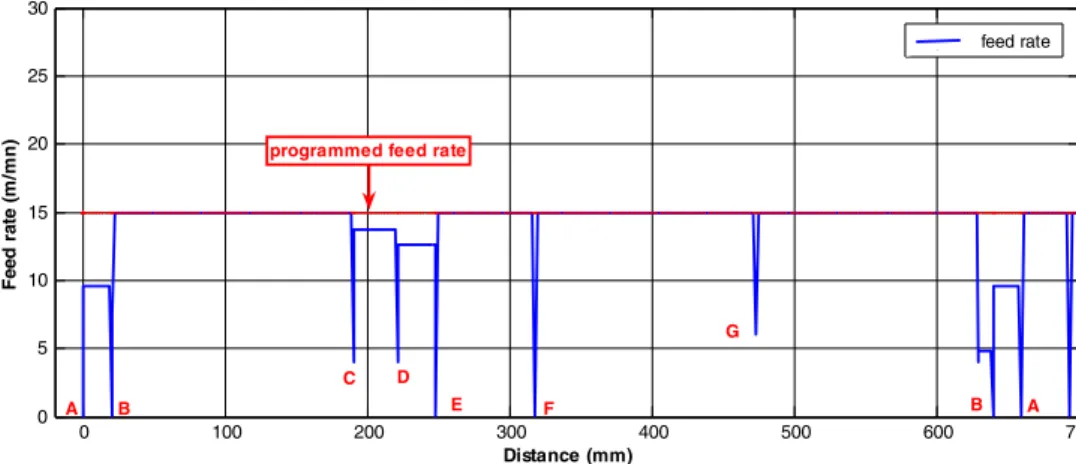
the trajectory ABCDEFG (Fig. 5) is shown in Fig. 6.

Then, for the same programmed feed rate (15 m/min), a comparison of the simulated profile with the experi-mental reading is realized (Fig.7).

The influence of the recent HSM machines dynamic behavior is to be noted. The feed rate profile (Fig. 6)

simulated on the path ABCDEFG (Fig.5) is very near

(2% of error) that of the experimental reading (Fig.7). In fact, the controller imposes these limitations accord-ing to the characteristics of the HSM machine axes and mainly to the maximal jerk.

Fig. 2 Tool path modelization by arc of circle [2]

Fig. 3 Calculation algorithm of the modified Static Look Ahead [6]

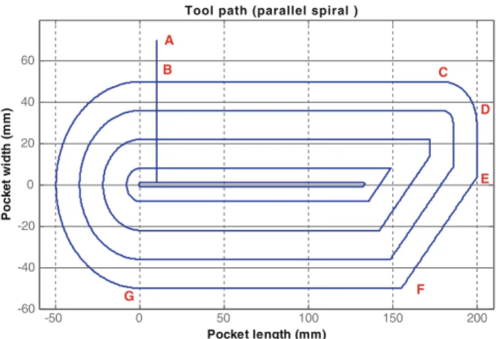
After that, the tool path is simulated with the con-vergent parallel spiral strategy, issued from a CAM Mastercam© solution (Fig.8), and also the correspon-dent simulated and experimental feed rate profiles of the pocket hollowing out (Figs.9and10).

5.2 Tool paths and feed rate profiles

In this section, concerning the pocket (Fig. 5), we get

interested in the simulation of the tool paths and the corresponding feed rate profiles for all the available strate-gies in Mastercam© CAM software. The simulations for the convergent parallel spiral strategy are mentioned before-hand, and here the simulations for another example of strategy are going to be presented.

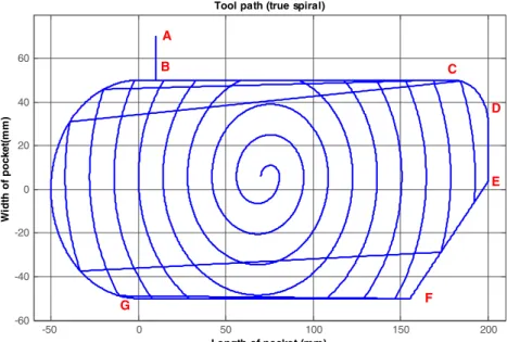
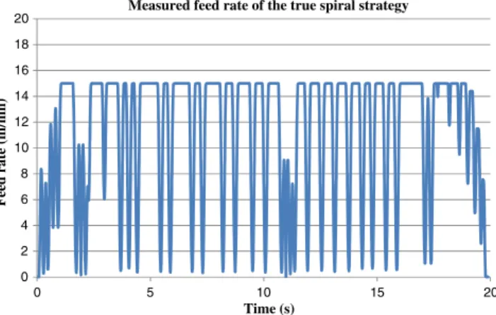
Strategy of the type: true spiral

The true spiral trajectory is a continuous curve connecting the geometry center and its periphery by a convergent spiral.

Figure 11 presents the tool path calculated on

Matlab©, in true spiral strategy.

Figure12presents the feed rate generated in dynamic look ahead for the true spiral strategy.

Figure13presents the feed rate profile read from the experiment of the pocket hollowing out with the true spiral strategy (Huron Kx 10).

The feed rate decreases progressively with the pro-gressive reducing of the path radii.

5.3 CAM paths analysis

5.3.1 Total length of the HSM path

The total length of the journey is a principal factor on the time cycle. The trajectories total lengths are compared in Fig.14in the frame of our pocket piece. Based only on the trajectory length and without taking into consideration the machine cinematic behavior, the most rapid strategies are the parallel spiral strategies of different types (divergent, convergent, and clean corners).

5.3.2 Use percentage of the recommended speed

If the trajectory total length criterion is linked to the average speed or to the use percentage of the programmed feed rate, we end in a global indicator of the machining time.

Figure 15 shows the use percentage of the recommended

Fig. 5 Trajectory and complex pocket [6] 0 100 200 300 400 500 600 700 0 5 10 15 20 25 30 Distance (mm) F e e d ra te ( m /m n

) _{programmed feed rate}

feed rate A B C D E F G B A

Fig. 6 Profile of the real feed rate simulated with the dynamic look ahead on the trajectory ABCDEFG

speed for each strategy. According to the figure, the most rapid strategies are those in true spiral strategy, and all types of parallel spiral strategies.

5.3.3 The length of segments

The length of segments is an interesting criterion for the trajectories, reserved to the HSM. The interpolation cycle time tcyis the necessary time for the controller to construct a segment of a minimal length. So, if the length of a segment between two blocks becomes too small, the controller recal-culates the feed rate (static look-ahead).

The interpolation cycle time of the NCU Siemens 840 D, identified by Tapie et al. [9, 10] is tcy0 12 ms. So, if the recommended feed rate is Vfprog0 15 m/min, dur-ing the interpolation cycle, the distance covered is L¼Vfprog&tcy

60 ¼ 3 mm:

So, for any block with a distance inferior to 3 mm, the feed rate will be limited. In HSM conditions, for the morph spiral strategy, if the distance to cover between two succes-sive information is inferior to 3 mm, then the simulated feed rate decreases to the minimal values to compensate the interpolation cycle time tcy.

Afterwards, if a strategy contains a great number of small segments, no doubt it becomes costly as far as the

machin-ing time is concerned. Figure 16 presents the number of

segments range of length for all strategies.

The three previous figures show that the morph spiral strategy generates many more small sized segments (inferior to 3 mm), then the constant overlap spiral strategy etc. They contain an important slowing factor considered costly for the machining time.

However, some strategies such as true spiral one also contain many more big sized segments (superior to 10 mm) without considering the intersections with the border of the piece. So, on these segments, the programmed speed can be reached and the average feed rate increases.

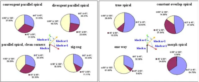
5.3.4 Change of direction

In HSM, the greater the radius of the arc, the more minimal the passage speed, consequently these radii must be opti-mized. In order to define these limitations, the percentage of the α angles must be calculated between two operations (or displacements). These angles can be found in three sectors for each strategy [3].

– _{The first sector, the most favorable, represents an angle} comprised in the range [0°, 45°],

– _{The second sector, which is costly, represents an angle}

comprised in the range [45°, 90°],

– _{The third sector, very costly, represents an angle in the} range [90°, 180°].

To evaluate the most costly strategies in accordance with this criterion, the changes of directions included in each

sector must be quantified. Figure17compares the changes

of direction carried out in accordance with the machining strategies of our study.

The morph spiral strategy is the most favorable for the changes of direction: 64.79% in the favorable sector. On the other hand, the one-way strategy generates the most uneven journey: 61.80% of change of direction in the very costly sector. However, this analysis does not make it possible to predict the most rapid strategy, for there must be a compro-mise between the different criteria. For example, the morph spiral strategy has the highest percentage of change of direction in the favorable sector, but it also has the greatest number of the small sized segments.

5.3.5 Conclusion of the geometrical analysis

Table1below sums up the strategies which seem to be the

most suitable through the criteria of the trajectories -5 0 5 10 15 20 25 0 0.5 1 1.5 2 2.5 3 3.5 4

Measured feed rate of the parallel spiral strategy

Time (s) Feed rate (m/mn) A B C D E F G B A

Fig. 7 Feed rateprofile read from the experiment

-50 0 50 100 150 200 -60 -40 -20 0 20 40 60 Pocket length (mm) P o c k e t w id th ( m m )

Tool path (parallel spiral )

A B C D E F G

geometrical analysis. In order to know the optimal strategy, the strategies must be then evaluated towards the machining time. This is the object of what follows.

5.4 Machining time simulation 5.4.1 CAM machining time

The estimation of the machining time in CAM, by the classical method, consists in dividing the total curvilinear length of the pocket hollowing-out trajectory by the programmed speed.

tFAO¼

Ltrj

Vprog

ð2Þ Without doubt, the results will be skewed because the dynamic factors have not been taken into account. The CAM calculation method largely underestimates the ma-chining time, when the trajectory is found to be complex and the recommended speed is high. In the literature, several models have been developed for machining real-time esti-mation. But these models do not integrate the interpolation cycle time, the look-ahead value, nor the jerk [2].

5.4.2 Machining time of the dynamic model

By using the previous simulations, the machining time which takes into account the previous dynamic criteria can be determined. Two different models have to be simulated to know about the effect of interpolation cycle time tcy. In the first, the time in static look ahead is simulated without considering the accelerations and the decelerations (time tLAS(i) (3)). In the second, the time in dynamic look ahead is simulated by taking into account the accelerations and the decelerations (time tLAD(i) (4)).

& Simulated times

The time models simulated on a block (i) with an ordinary speed profile (Fig.18) are:

– _{The time LASon a block (i) is equal to the length of the} block divided by the stationary speed of this block, not considering the variation during the acceleration or during the deceleration.

tLASðiÞ ¼

LðiÞ VstationaryðiÞ

ð3Þ

– _{The time LADon a block (i) is equal to the sum of the}

acceleration time tacc, the stationary time tstat (at the

stationary speed Vstat (i)m/min) and the deceleration

time tdec

tLADðiÞ ¼ taccðiÞ þ tstatðiÞ þ tdecðiÞ ð4Þ

The acceleration time tacc(i) is equal to the interpolation cycle time tcy.

taccðiÞ ¼

daccðiÞ VstatðiÞ # Vstatði# 1Þ

¼ tcy with tcy¼ 12 ms ' ( : ð5Þ 0 500 1000 1500 2000 0 5 10 15 20 25 30 Distance (mm) F e e d r a te ( m /m n

) programmed feed rate

feed rate A B C D E F G B A

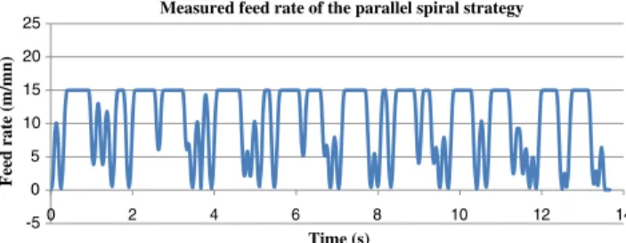
Fig. 9 Profile of the real feed rate simulated all over the pocket for a 15 m/min programmed feed rate (Huron Kx 10) -5 0 5 10 15 20 25 0 2 4 6 8 10 12 14

Measured feed rate of the parallel spiral strategy

Time (s)

Feed

rate

(m/mn)

Fig. 10 Feed rate profile read from the experiment of the pocket hollowing out with the parallel spiral strategy

The stationary time tstat (i) is given by the following expressions, according to the stationary speeds of the current, the next and the previous blocks.

tstatðiÞ ¼

LðiÞ # ddecðiÞ # daccðiÞ

VstatðiÞ

if VstatðiÞ > Vstatði # 1Þ and VstatðiÞ > Vstatði þ 1Þ

LðiÞ # ddecðiÞ

VstatðiÞ

if VstatðiÞ < Vstatði # 1Þ and VstatðiÞ > Vstatði þ 1Þ

LðiÞ # daccðiÞ

VstatðiÞ

if VstatðiÞ > Vstatði # 1Þ and VstatðiÞ < Vstatði þ 1Þ

LðiÞ VstatðiÞ else 8 > > > > > > > > > > > > < > > > > > > > > > > > > : ð6Þ -50 0 50 100 150 200 -60 -40 -20 0 20 40 60 Length of pocket (mm) W id th o f p o c k e t( m m )

Tool path (true spiral)

A B C D E F G

Fig. 11 True spiral trajectory for the test pocket

0 500 1000 1500 2000 2500 3000 3500 4000 0 2 4 6 8 10 12 14 16 18 20 Distance (mm) F e e d r a te ( m /m n )

programmed feed rate

feed rate

Fig. 12 True spiral feed rate simulated for the test pocket

The deceleration time tdec (i) is equal to the interpola-tion cycle time tcy.

tdecðiÞ ¼

ddecðiÞ

VstatðiÞ # Vstatðiþ 1Þ

¼ tcy ð7Þ

Hence, the dynamic look ahead time tLADis given by the following equations:

tLADðiÞ ¼

LðiÞ # ddecðiÞ # daccðiÞ

VstatðiÞ

þ2 & tcy if VstatðiÞ > Vstatði # 1Þ and VstatðiÞ > Vstatði þ 1Þ

LðiÞ # ddecðiÞ

VstatðiÞ

þtcy if VstatðiÞ < Vstatði # 1Þ and VstatðiÞ > Vstatði þ 1Þ

LðiÞ # daccðiÞ

VstatðiÞ

þtcy if VstatðiÞ > Vstatði # 1Þ and VstatðiÞ < Vstatði þ 1Þ

LðiÞ VstatðiÞ else 8 > > > > > > > > > > > > < > > > > > > > > > > > > : ð8Þ

& Real-time evolution (tLAD) for each strategy

The simulation for an example of strategy is presented.

– _{One way}

The pocket hollowing out total time of the one way strategy is equal to 33.30 s. It is important because the trajectory length is very critical.

5.4.3 Conclusion of the machining time analysis

Table 2 below sums up the hollowing out time of the

test pocket (CAM, simulated and measured LAD on HSM machine Huron KX10) according to the hollowing

out geometrical strategies generated in CAM. If a strat-egy block number is low (59 blocks for parallel spiral), one notices that there is not a great influence of the accelerations and of the decelerations upon the machin-ing time (of the order of 0.09 s). Nevertheless, if the number of blocks is important (3,228 blocks for morph spiral), they have a considerable influence. Thus, it is also possible to notice the influence of the machine dynamics more clearly, by calculating the gap between the simulated real machining time (tLAD) and the CAM time (tCAM) for each strategy.

Figure 19 shows the gap (%) between the CAM

time and the experimental or the simulated time LAD. The gaps are variable and indicate that the most costly strategy for the dynamics of the machine is the morph spiral. Whereas, the least costly one is the true spiral.

That gap informs us about the dynamic behavior criterion of the machine for each strategy, but it does not allow us to state that the true spiral (19.42%) is the optimal strategy, because the trajectory total length is important enough (3.99 m), compared with the others which also have small gaps like the divergent parallel spiral (1.98 m, 41.73%). Hence, the machining time is the principal criterion which will inform us about the optimal strategy.

The most appropriate strategy as far as the machining time is concerned, is the divergent parallel spiral strategy. It is then the optimal strategy towards the dynamic behavior of the HSM machine and the machining time. This result is similar to that of Duc et al. [1], which refers to the optimal strategy for the closed pockets machining.

0 2 4 6 8 10 12 14 16 18 20 0 5 10 15 20 Feed rate (m/mn) Time (s)

Measured feed rate of the true spiral strategy

Fig. 13 Feed rate profile read from the experiment of the pocket hollowing out with the true spiral strategy

59.94 79.4 75.66 72.68 82.97 11.79 35.77 60.74 0 10 20 30 40 50 60 70 80 90 percentage (%)

Use percentage of the programmed feed rate

zig-zag

convrergent parallel spiral divergent parallel spiral parallel spiral,clean corners true spiral

morph spiral one way

constant overlap spiral

Fig. 15 Use percentages of the programmed feed rate, Vprog0 15 m/min

Fig. 16 Number of segments by range of length for all machines strategies 3.80 2.02 1.98 2.07 3.99 3.76 6.14 2.25 0 1 2 3 4 5 6 7 Length in m Trajectories lengths zig-zag

convergent parallel spiral divergent parallel spiral parallel spiral,clean corners true spiral

morph spiral one way

constant overlap spiral

Fig. 14 Comparison of trajecto-ries lengths

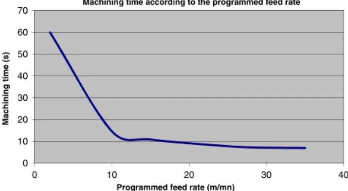
5.4.4 Influence of the programmed speed upon the machining time

According to the optimal strategy, the programmed feed rate undergoes a variation making it possible to know the influence of this variation upon the machining time

(simulations in HSM machine Mikron case). Table 3

presents the simulated programmed speeds. Figure 20

presents the machining time variation according to the programmed feed rate.

It is to note that the machining time records an important diminution of 60–10 s by increasing the feed rate from 2 to 10 m/min. After that, from 10 to 27 m/ min, the diminution becomes small from 10 to 7 s. Finally, the machining time becomes asymptotic regard-less of the programmed feed rate. Subsequently, it

becomes possible to conclude that increasing the

programmed feed rate doesn’t always mean the machin-ing time diminution, but this feed rate must be opti-mized according to the machine cinematic capabilities.

Figure 21presents the use percentage of the programmed

feed rate for each simulation test (Table3).

The percentage of the programmed feed rate utiliza-tion decreases in a regular way from 73.56% to 64.69%

by increasing the feed rate from 2 to 29 m/min, as long as the feed rate remains in the range of the HSM machine axes capabilities. However, it diminishes by reaching 5.51% for 35 m/min, because the maximal feed rates of the machine axes (30 m/min X, Y, Z) are outdone.

6 Conclusion

In this article, we have been interested in the tool trajectories simulation of a test pocket hollowing out, for the strategies generated in CAM, as well as in the feed rate profiles by applying the dynamic models de-veloped in the first part.

Afterwards, the analysis of the factors having an influence upon the cycle time has been mentioned. First, each trajectory total length has been calculated. Then, other criteria are developed like the number of small segments and the percentage of the unfavorable angles for each strategy.

Then, we presented the simulation of the machining time generated by the CAM tool and the real-time

Fig. 17 The changes of direction carried out in accordance with strategies

Table 1 Strategies adapted to the stated criteria Criterion Total length Use percentage

of Vprog Segment length Change of direction Strategy Divergent parallel spiral

True spiral True spiral Morph spiral

dacc (i)

Vstat (i) -V (i+1)

Block (i) L (i) ddec(i) Block (i+1) L (i+1) Block (i-1) L (i-1) Vstat (i-1) Vstat (i+1) Vstat (i)

Vstat(i) -V (i-1)

Vstationary (i)

simulated by taking or not the accelerations and the decelerations into account. It is noticed that the optimal strategy is the one in divergent parallel spiral in the case of our test piece "pocket" and that the most costly strategy for the machine dynamic behavior is the one in morph spiral.

At last, we have tried to know the influence of the programmed feed rate. So, it is possible to conclude that the increasing of the feed rate does not always mean the machining time diminution. Hence, the opti-mal feed rate which considers the overload of the HSM machine must be chosen, in other words, the pocket machining optimization, according to the strategy and the feed rate.

Table 2 The pocket hollowing

out time by strategies Zigzag (s) Convergent parallel

spiral (s) Divergent parallel spiral (s) Parallel spiral, clean corners (s) CAM Time 15.19 8.07 7.93 8.28 LAD Time 25.66 14.12 14.22 17.23

LAD experimental time 22.94 13.84 13.61 15.12

True spiral Constant overlap spiral Morph spiral One way

CAM time 15.97 9.00 15.04 24.56

LAD time 21.72 21.24 207.91 33.30

LAD experimental time 19.82 17.34 32.72 31.00

0.00% 20.00% 40.00% 60.00% 80.00% 100.00% measured simulated

Fig. 19 Gap (%) between the CAM time and the dynamic time

0 10 20 30 40 50 60 70 0 10 20 30 40 Machining time (s)

Programmed feed rate (m/mn)

Machining time according to the programmed feed rate

Fig. 20 Machining time variation according to the programmed feed rate

73.56% 72.44% 69.24% 65.24% 64.69% 5.51%

Use percentage of the programmed feed rate 1 2 3 4 5 6 2 m/min 10 m/min 15 m/min 25 m/min 29 m/min 35 m/min

Fig. 21 Use percentage of the programmed feed rate for each simula-tion test

Table 3 Simulated programmed speeds

Test N° 1 2 3 4 5 6

References

1. Duc E, Geiskopf F, Landon Y (1999) The high speed milling. ENS of Cachan (LURPA), France

2. Dugas A. (2002) CFAO et UGV: machining simulation of the complex forms. Doctoral thesis. Central School of Nantes, France. 3. Mawussi K, Lavernhe S, Lartigue C (2003) HSM machining pockets: help in choosing strategies. Int J CAD/CAM Comp Grap 18(3):337–349

4. Mehdi C. (2000) Reconstruction of a CAD model from the real movements of a machine TM/NC. Memory of master, IRCCyN. Central School of Nantes, France.

5. Monreal M, Rodriguez CA (2001) Influence of tool path strategy on the cycle time of high speed milling. Int J Comp Aid Des 35:395–401

6. Msaddek EB, Bouaziz Z, Baili M, Dessein G (2011) Modeling and simulation of high-speed milling centers dynamics. Int J Adv Manu Tech 53(9–12):877–888

7. Pateloup V, Duc E, Pascal R (2004) Corner optimization for pocket machining. Int J Mach Tools Manu 44:1343–1353

8. Pateloup V., Duc E. et Ray P. (2003) Optimization of the pockets hollowing out trajectories for the high speed milling. 16th French Congress of Mechanics, Nice, pp. 1–6.

9. Tapie L, Mawussi KB, Anselmetti B (2006) Machining strategy choice: performance viewer. CDRom paper IDMME 2006, Grenoble, France. pp. 17–19

10. Tapie L, Mawussi KB, Anselmetti B (2006) Circular tests for HSM machine tools: bore machining application. Int J Mach Tools Manu 47:805–819

11. Toh CK (2004) Design, evaluation and optimization of cutter path strategies when high speed machining hardened die and mold materials. Int J Mat Des 26:517–533

12. Toh CK (2004) Cutter path strategies in high speed rough milling of hardened steel. Int J Mat Des 27:107–114

13. Tournier C, Lavernhe S, Lartigue C (2005) Optimization in 5-axis high speed milling. CDRom paper. CPI'2005 Casablanca, Morocco. pp. 1–11.