Bootstrap Methods for Factor Models
par
Antoine A. Djogbenou
Département de sciences économiques
Faculté des arts et sciences
Thèse présentée à la Faculté des études supérieures
en vue de l’obtention du grade de Philosophiæ Doctor (Ph.D.)
en sciences économiques
Juillet, 2016
Cette thèse intitulée :
Bootstrap Methods for Factor Models
présentée par :
Antoine A. Djogbenou
a été évaluée par un jury composé des personnes suivantes :
William McCausland, président-rapporteur
Benoit Perron,
directeur de recherche
Sílvia Gonçalves,
co-directrice de recherche
Marine Carrasco,
membre du jury
Xu Cheng,
examinatrice externe
Jacques Bélair,
vice-doyen, représentant du doyen de la FAS
Dédicace iii
Remerciements iv
Résumé v
Abstract vii
Table des matières viii
Liste des figures viii
Liste des tableaux viii
Introduction Générale 1
1 Bootstrap Inference in Regressions with Estimated Factors and Serial
Cor-relation 3
1.1 Introduction . . . 3
1.2 Assumptions and asymptotic results . . . 4
1.3 Bootstrap inference . . . 8
1.3.1 General residual-based bootstrap : review . . . 8
1.3.2 Block wild bootstrap . . . 9
1.3.3 Dependent wild bootstrap . . . 10
1.4 Simulation results . . . 11
2 Bootstrap Prediction Intervals for Factor Models 14 2.1 Introduction . . . 14
2.2 Prediction intervals based on asymptotic theory . . . 16
2.2.1 Assumptions . . . 16
2.2.2 Normal-theory intervals . . . 17
2.3 Description of bootstrap intervals . . . 19
2.4 Bootstrap distribution of estimated factors . . . 22
2.5 Validity of bootstrap intervals . . . 25
2.5.1 Confidence intervals for yT +1|T . . . 25
2.5.2 Prediction intervals for yT +1 . . . 26
2.5.3 Multi-horizon forecasting, h > 1 . . . 28
2.6 Simulations . . . 29
2.6.1 Forecasting horizon h = 1 . . . 31
2.6.2 Multi-horizon forecasting . . . 33
2.7 Empirical illustration . . . 35
2.8 Conclusion . . . 38
3 Model Selection in Factor-Augmented Regressions with Estimated Factors 39 3.1 Introduction . . . 39
3.2 Settings and assumptions . . . 41
3.3 Model selection . . . 43
3.3.1 Leave-d-out or delete-d cross-validation . . . 44
3.3.2 Bootstrap rule for model selection . . . 49
3.4 Simulation experiment . . . 51
3.5 Empirical application . . . 55
3.5.1 In-sample prediction of excess returns . . . 57
3.5.2 Out-of-sample prediction of excess returns . . . 57
3.6 Conclusion . . . 59
Conclusion générale 60 Annexes 65 .1 Proofs of results in Sections 1.2 and 1.3 . . . 65
.2 Proofs of results in Chapter 2 . . . 76
.3 Proofs of results in Chapter 3 . . . 82
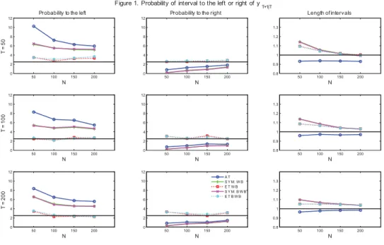
Figure 1. Probability of interval to the left or the right of yT +1|T . . . 31
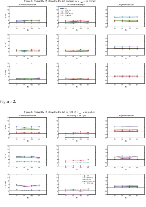
Figure 2. Probability of interval to the left or the right of yT +1, epsilon is normal . . . 32
Figure 3. Probability of interval to the left or the right of yT +1, , epsilon is mixture . 33 Figure 4. Probability of interval to the left or the right of yT +4|T . . . 33
Figure 5. Probability of interval to the left or the right of yT +4, epsilon is normal . . . 34
Figure 6. Probability of interval to the left or the right of yT +4, epsilon is mixture . . 35
Figure 7. Prediction interval for changes in the inflation rate-Factor-augmented fore-cast intervals . . . 36
Figure 7. Prediction interval for 2008 and 2011 . . . 37
Figure 9. Frequencies of selecting a larger set of estimated factors minimizing the CV1, the CV1 without the factor estimation error and the CV1 without the parameter and the factor estimation errors over 10,000 simulations . . . 47
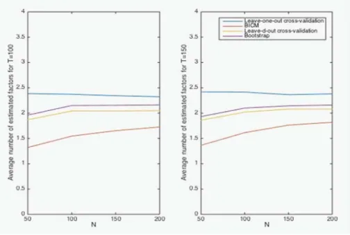
Figure 10. Average parameter estimation error and factor estimation error in the CV1 47 Figure 11. Average number of estimated factors for DGP 1 . . . 53
Figure 12. Average number of estimated factors for DGP 2 . . . 53
Figure 12. Average number of estimated factors for DGP 3 . . . 54
Figure 14. Frequencies of selecting the two first estimated fators for DGP 1 . . . 54
Figure 15. Frequencies of selecting the three first estimated fators for DGP 2 . . . 55
Figure 16. Frequencies of selecting the four estimated fators for DGP 3 . . . 55
Figure 17. Number of selected factors in the out-of-sample exercise . . . 58
Table 1. Simulation results . . . 12 Table 2 : Variation explained by estimated macro and financial factors . . . 101 Table 3 : Estimation results . . . 101
Remerciements
J’ai un devoir de reconnaissance à l’endroit de mes directeurs de thèse, Sìlvia Gonçalves et Benoit Perron que j’exprime sincèrement ici. Je leur serai toujours redevable pour leur disponi-bilité, leur implication et leur soutien, tout au long de ce cheminement de doctorat. Travailler avec eux a été très enrichissant pour moi et j’espère vivement pouvoir continuer à apprendre d’eux dans les années à venir.
Ma reconnaissance infinie va à l’endroit de tout le corps professoral du Département de sciences économiques de l’Université de Montréal pour tout ce que j’ai appris d’eux. Elle va en particulier à Marine Carrasco qui me suit depuis la première présentation orale de cette thèse. Je remercie également le personnel administratif du département pour leur disponibilité sans cesse renouvelée.
J’adresse mes sincères remerciements à Guy Tchuente, Juste Somé, Idrissa Ouili et William Gbohoui pour avoir été présents pour moi dès mes débuts à Montréal et à Mohamed Doukali pour sa grande amitié. Je voudrais dire un grand merci à Désiré Kédagni, pour avoir rêvé ensemble depuis notre premier cycle d’aller aussi loin que possible et relevé ensemble les défis qui se sont présentés à nous. Mes chaleureux remerciements vont à l’endroit de mes nombreux collègues et amis de l’Université de Montréal que je ne pourrai tous citer ici pour les discussions instructives et les bons moments passés ensembles.
À ma mère et mes sœurs pour qui ces cinq années de thèse ont sans doute paru longues, je suis reconnaissant pour le soutien moral continu. A ma merveilleuse épouse Mariam, je témoigne ma profonde gratitude pour sa grande compréhension, sa patience et surtout pour avoir été ce support sur lequel je pouvais m’appuyer quand tout semblait s’écrouler autour de moi.
Ce cheminement n’aurait pas été possible sans le soutien financier du Département de Sciences Économiques de l’Université de Montréal, le Centre Interuniversitaire de Recherche en Économie Quantitative (CIREQ) et la Faculté des Études Supérieures et Postdoctorales que je remercie ici.
Résumé
Cette thèse développe des méthodes bootstrap pour les modèles à facteurs qui sont couram-ment utilisés pour générer des prévisions depuis l’article pionnier de Stock et Watson (2002) sur les indices de diffusion. Ces modèles tolèrent l’inclusion d’un grand nombre de variables macroéconomiques et financières comme prédicteurs, une caractéristique utile pour inclure di-verses informations disponibles aux agents économiques. Ma thèse propose donc des outils éco-nométriques qui améliorent l’inférence dans les modèles à facteurs utilisant des facteurs latents extraits d’un large panel de prédicteurs observés. Il est subdivisé en trois chapitres complémen-taires dont les deux premiers en collaboration avec Sílvia Gonçalves et Benoit Perron.
Dans le premier article, nous étudions comment les méthodes bootstrap peuvent être utilisées pour faire de l’inférence dans les modèles de prévision pour un horizon de h périodes dans le futur. Pour ce faire, il examine l’inférence bootstrap dans un contexte de régression augmentée de facteurs où les erreurs pourraient être autocorrélées. Il généralise les résultats de Gonçalves et Perron (2014) et propose puis justifie deux approches basées sur les résidus : le block wild bootstrap et le dependent wild bootstrap. Nos simulations montrent une amélioration des taux de couverture des intervalles de confiance des coefficients estimés en utilisant ces approches comparativement à la théorie asymptotique et au wild bootstrap en présence de corrélation sérielle dans les erreurs de régression.
Le deuxième chapitre propose des méthodes bootstrap pour la construction des intervalles de prévision permettant de relâcher l’hypothèse de normalité des innovations. Nous y propo-sons des intervalles de prédiction bootstrap pour une observation h périodes dans le futur et sa moyenne conditionnelle. Nous supposons que ces prévisions sont faites en utilisant un ensemble de facteurs extraits d’un large panel de variables. Parce que nous traitons ces facteurs comme latents, nos prévisions dépendent à la fois des facteurs estimés et les coefficients de régres-sion estimés. Sous des conditions de régularité, Bai et Ng (2006) ont proposé la construction d’intervalles asymptotiques sous l’hypothèse de Gaussianité des innovations. Le bootstrap nous permet de relâcher cette hypothèse et de construire des intervalles de prédiction valides sous des hypothèses plus générales. En outre, même en supposant la Gaussianité, le bootstrap conduit à des intervalles plus précis dans les cas où la dimension transversale est relativement faible car il prend en considération le biais de l’estimateur des moindres carrés ordinaires comme le montre une étude récente de Gonçalves et Perron (2014).
Dans le troisième chapitre, nous suggérons des procédures de sélection convergentes pour les regressions augmentées de facteurs en échantillons finis. Nous démontrons premièrement que la méthode de validation croisée usuelle est non-convergente mais que sa généralisation, la validation croisée «leave-d-out» sélectionne le plus petit ensemble de facteurs estimés pour l’espace généré par les vraies facteurs. Le deuxième critère dont nous montrons également la validité généralise l’approximation bootstrap de Shao (1996) pour les regressions augmentées
de facteurs. Les simulations montrent une amélioration de la probabilité de sélectionner par-cimonieusement les facteurs estimés comparativement aux méthodes de sélection disponibles. L’application empirique revisite la relation entre les facteurs macroéconomiques et financiers, et l’excès de rendement sur le marché boursier américain. Parmi les facteurs estimés à partir d’un large panel de données macroéconomiques et financières des États Unis, les facteurs fortement correlés aux écarts de taux d’intérêt et les facteurs de Fama-French ont un bon pouvoir prédictif pour les excès de rendement.
Mots-clés : Modèles à facteurs, correlation sérielle, prévision, moyenne conditionnelle, sélec-tion de modèle, validasélec-tion croisée, bootstrap, inflasélec-tion, excès de rendement boursier, É.U.
Abstract
This thesis develops bootstrap methods for factor models which are now widely used for generating forecasts since the seminal paper of Stock and Watson (2002) on diffusion indices. These models allow the inclusion of a large set of macroeconomic and financial variables as predictors, useful to span various information related to economic agents. My thesis develops econometric tools that improves inference in factor-augmented regression models driven by few unobservable factors estimated from a large panel of observed predictors. It is subdivided into three complementary chapters. The two first chapters are joint papers with Sílvia Gonçalves and Benoit Perron.
In the first chapter, we study how bootstrap methods can be used to make inference in h-step forecasting models which generally involve serially correlated errors. It thus considers bootstrap inference in a factor-augmented regression context where the errors could potentially be serially correlated. This generalizes results in Gonçalves and Perron (2013) and makes the bootstrap applicable to forecasting contexts where the forecast horizon is greater than one. We propose and justify two residual-based approaches, a block wild bootstrap (BWB) and a dependent wild bootstrap (DWB). Our simulations document improvement in coverage rates of confidence intervals for the coefficients when using BWB or DWB relative to both asymptotic theory and the wild bootstrap when serial correlation is present in the regression errors.
The second chapter provides bootstrap methods for prediction intervals which allow re-laxing the normality distribution assumption on innovations. We propose bootstrap prediction intervals for an observation h periods into the future and its conditional mean. We assume that these forecasts are made using a set of factors extracted from a large panel of variables. Because we treat these factors as latent, our forecasts depend both on estimated factors and estimated regression coefficients. Under regularity conditions, Bai and Ng (2006) proposed the construction of asymptotic intervals under Gaussianity of the innovations. The bootstrap al-lows us to relax this assumption and to construct valid prediction intervals under more general conditions. Moreover, even under Gaussianity, the bootstrap leads to more accurate intervals in cases where the cross-sectional dimension is relatively small as it reduces the bias of the ordinary least squares estimator as shown in a recent paper by Gonçalves and Perron (2014).
The third chapter proposes two consistent model selection procedures for factor-augmented regressions in finite samples. We first demonstrate that the usual cross-validation is inconsistent, but that a generalization, leave-d-out cross-validation, selects the smallest basis of estimated factors for the space spanned by the true factors. The second proposed criterion is a genera-lization of the bootstrap approximation of the squared error of prediction of Shao (1996) to factor-augmented regressions which we also show is consistent. Simulation evidence documents improvements in the probability of selecting the smallest set of estimated factors than the usually available methods. An illustrative empirical application that analyzes the relationship
between expected stock returns and macroeconomic and financial factors extracted from a large panel of U.S. macroeconomic and financial data is conducted. Our new procedures select fac-tors that correlate heavily with interest rate spreads and with the Fama-French facfac-tors. These factors have strong predictive power for excess returns.
Keywords : Factor model, serial correlation, forecast, conditional mean, model selection, cross-validation, bootstrap, excess returns, U.S.
Introduction Générale
Dans les dernières décennies, nous avons noté une disponibilité croissante de données éco-nomiques. Leur utilisation pour générer des prévisions a connu un regain d’intérêt depuis le travail pionnier de Stock et Watson (2002) sur les modèles à facteurs augmentés. Ces modèles assument que la variable d’intérêt par exemples l’inflation ou l’excès de rendement boursier dépendent non seulement de variables observées mais aussi de facteurs inobservés résumant l’information d’un grand nombre de variables.
En pratique, parce que les facteurs sont latents, ils sont remplacés par leur version estimée généralement par la méthode des composantes principales. Sous des conditions de régularité, Bai et Ng (2006) montrent que les facteurs extraits peuvent être traités comme si ils éntait observés lorsque la racine carrée de la dimension temporelle sur le nombre de série tend vers zéro. En examinant les propriétés asymptotiques, Gonçalves et Perron (2014) démontrent la présence d’un biais dans la distribution asymptotique de l’estimateur obtenu par la regression augmentée de facteurs. De surcroît, ils suggèrent une méthode de bootstrap en deux étapes permettant de capturer ce biais. Cette méthode du wild bootstrap détruit toute dépendance entre les observations. Ainsi, elle n’est valide que lorsque l’horizon de prévision est 1 car lorsque l’horizon de prévision est supérieure à une période, les innovations sont généralement dépendantes. Ce qui rend invalide le wild bootstrap. Dans le premier chapitre, nous justifions théoriquement la validité du block wild bootstrap et le dépendent wild bootstrap. Ces deux méthodes basées sur les résidus en dimension temporelle se rejoignent sur le fait qu’elles préservent la dépendance dans la variance asymptotique de l’estimateur. Toutefois, la première préserve cette dépendance en considérant k blocs de résidus multipliés chacun par une même variable externe. La seconde approche quant à elle lisse les variables externes au delà des blocs.
Dans le deuxième chapitre, nous justifions la validité du bootstrap pour construire les in-tervalles de prédiction pour une réalisation future de la variable dépendante ou sa moyenne conditionnelle à l’information disponible. Nos résultats, permettent contrairement à l’approache asymptotique usuelle, de relâcher l’hypothèse de normalité des innovations futures. En appli-quant notre demarche à la prévision des changements de l’inflation avec des données trimes-trielles de l’économie américaine couvrant la période 1973 à 2014, nos intervalles de prédiction incluent la forte déflation observée pendant la crise financière de 2008 et celle du dernier tri-mestre de 2011.
Nous complètons notre analyse dans le troixième chapitre par l’examen du choix des facteurs estimés à inclure dans l’équation de prévision. En effet, les facteurs latents F0 importants pour prédire la variable dépendente ne sont pas nécessairement tous ceux (F ) qui résument l’infor-mation dans le grand nombre de prédicteurs disponibles X. Nous nous fixons comme objectif de détecter le plus petit ensemble de regresseurs générés capable de recouvrir l’information dans F0. Bien que beaucoup de travaux se sont intéressé au choix des facteurs estimés reflétant
le mouvement commun dans X, peu se sont penchés sur l’identification de ces derniers. Nous explorons comment la méthode de validation croisée peut être utilisée dans notre contexte de régresseurs générés. Nous montrons que la méthode de sélection de validation croisée usuelle n’est valide que lorsqu’un seul ensemble de facteurs estimés est correct. Pour remédier à cette situation, nous justifions la validité du «leave-d-out cross-validation» avec un d convenablement choisi. Nous proposons également une approche de bootstrap convergente qui contrairement à la méthode de validation croisée leave-d-out évalue l’habileté de prédiction des modèles can-didats avec un estimateur se basant sur toutes les observations. En considérant un ensemble de 277 variables macroéconomiques et financières, nous avons étudié les déterminants de l’ex-cès de rendement boursier sur le marché américain en revisitant le travail de Ludvigson et Ng (2007). Les facteurs fortement correlés aux écarts entre les taux d’intérêts et le taux directeur et les facteurs de Fama-French ont un fort pouvoir prédictif pour l’excès de rendement boursier. Nos résultats montrent que les approches suggérées protègent contre la sélection d’un nombre inapproprié de facteurs estimés.
Chapitre 1
Bootstrap Inference in Regressions
with Estimated Factors and Serial
Correlation
1.1
Introduction
Factor-augmented regressions have become quite popular in research in finance and econo-mics since the seminal paper of Stock and Watson (2002). They are often used in a forecasting context as they allow to summarize a large number of predictors with a small number of indexes. Because these indexes are treated as latent factors in an approximate factor model, the estimated regression contains estimated regressors which poses challenges for inference. Under regularity conditions, Bai and Ng (2006) derived the asymptotic distribution of regression esti-mates. One of the key conditions used in their work is that √T /N → 0. In that case, the error in estimating the factors can be neglected and inference can proceed as if they were observed.
Gonçalves and Perron (2014) (GP (2014) thereafter) showed that the finite sample properties of the asymptotic approach of Bai and Ng (2006) can be poor, especially if N is not sufficiently large relative to T . In particular, estimation of factors leads to an asymptotic bias term in the OLS estimator if √T /N → c and c = 0. They provided a set of high level conditions under which any residual-based bootstrap method is valid in this context and showed that a bootstrap algorithm based on the wild bootstrap removes this bias and outperforms the asymptotic approach of Bai and Ng (2006) in simulation experiments. This wild bootstrap algorithm is only valid when the forecasting horizon is one because it does not reproduce serial correlation. In general, when the forecasting horizon is larger than one and the model is correctly specified, the residuals in the factor-augmented regression will follow a moving average process (Diebold (2007), pp. 256-257).
In this paper, we extend the work of Bai and Ng (2006) and GP (2014) by considering errors
This chapter is a joint paper with Sílvia Gonçalves and Benoit Perron. The authors are grateful for comments from seminar participants at the Toulouse School of Economics, Pompeu Fabra University and Duke University, as well as from participants at the Workshop on Bootstrap Methods for Time Series, Copenhagen, Denmark, September 2013, and the MAESG conference in Emory, Atlanta, November 2013. Gonçalves acknowledges financial support from the NSERC and MITACS whereas Perron acknowledges financial support from the SSHRC and MITACS. We acknowledge that this chapter has been published by Journal of Time Series Analysis and agree with the publication disclosure.
that are serially correlated. Bai and Ng effectively ruled out possible serial correlation since their estimator of the asymptotic variance of the scaled average of the scores is only consistent with heteroskedasticity. We begin by providing an asymptotic theory under general assumptions on the serial correlation of the error term (of the strong mixing type) and proposing a consistent estimator of the covariance matrix in that case. As in GP (2014), we allow √T /N → c > 0 so that a bias term appears in the asymptotic distribution. Secondly, we propose two residual-based bootstrap schemes and show that they provide valid inference in this context. The first scheme which we call the block wild bootstrap (BWB) was proposed by Yeh (1998) for a linear regression with fixed scalar regressor and strong mixing errors. It is implemented by separating the residuals into non-overlapping blocks of observations and multiplying the elements of each block by the same realization of an external variable. The fact that each element in a block is multiplied by the same external draw generates correlation among the elements within a block but enforces independence across blocks. The second scheme we consider is the dependent wild bootstrap (DWB) originally proposed by Shao (2010) in the context of the smooth function model with time series observations. The DWB differs from the BWB by smoothing the external draws across blocks. Our main contribution is to show that these two methods are valid in the context of a factor augmented regression model with estimated factors and serially correlated errors, characterized by a strong mixing assumption.
The remainder of the paper is organized as follows. Section 1.2 introduces our assump-tions, provides the asymptotic distribution of the OLS estimator, and proposes a consistent estimator of the covariance matrix. Section 1.3 considers bootstrap inference using our two pro-posed algorithms. Section 1.4 presents our simulation experiments, and Section 1.5 concludes. Mathematical proofs appear in the Appendix 0.1.
1.2
Assumptions and asymptotic results
We consider the following standard factor-augmented regression model, yt+h = α Ft+ β Wt+ εt+h, t = 1, . . . , T − h,
where yt+h denotes the variable of interest, for example GDP growth or inflation, with h the forecast horizon. The r × 1 vector Ft consists of latent factors which help forecast yt+h. These are thought as common latent factors in a panel factor model given by
Xit = λiFt+ eit, i = 1, . . . , N, t = 1, . . . , T,
where λi, i = 1, . . . , N, are the r × 1 factor loadings and eit is an idiosyncratic error term, i = 1, . . . , N, t = 1, . . . , T. The vector Wt contains a smaller set of other observed regressors (including for instance a constant and lags of yt). We will denote the set of regressors as zt = (Ft, Wt) , t = 1, . . . , T.
We impose the following assumptions. Throughout, M = (trace (M M ))1/2 denotes the Euclidean norm, M > 0 denotes positive definiteness for a square matrix, and C represents a generic finite constant.
Assumption 1 (factor model) a) E Ft
4
≤ C and ΣF = limT →∞E (T−1F F ) = limT →∞E T−1 T
b) λi ≤ C if λi are deterministic, or E λi ≤ C if not, and N−1Λ Λ = N−1 N
i=1λiλi →P ΣΛ> 0.
c) The eigenvalues of the r × r matrix (ΣF × ΣΛ)are distinct. Assumption 2 (Idiosyncratic errors)
a) E (eit) = 0, E|eit|8 ≤ C.
b) E (eitejs) = σij,ts, |σij,ts| ≤ σijfor all (t, s) and |σij,ts| ≤ τstfor all (i, j) with N−1 N
i,j=1σij ≤ C, T−1 Tt,s=1τst ≤ C and (NT )−1 i,j,t,s=1|σij,ts| ≤ C.
c) E N−1/2 N
i=1(eiteis− E (eiteis)) 4
≤ C for all (t, s) .
Assumption 3 (Moments and weak dependence among {zt}, {λi}, and {eit})
a) E N−1 N
i=1 T−1/2 T
t=1Fteit 2
≤ C, where E (Fteit) = 0 for every (i, t) . b) For each t, E (N T )−1/2 Ts=1 Ni=1zs(eiteis− E (eiteis))
2
≤ C where zs = (Fs, Ws) . c) E (N T )−1/2 Tt=1ztetΛ
2
≤ C where E (ztλieit) = 0 for all (i, t) . d) E T−1 T
t=1 N−1/2 N i=1λiet
2
≤ C where E (λieit) = 0 for all (i, t) .
e) As N, T → ∞, (NT )−1 Tt=1 Ni=1 Nj=1λiλjeitejt−Γ →P 0,where Γ ≡ limN, T →∞T−1 Tt=1Γt> 0, and Γt≡ V ar N−1/2
N
i=1λieit .
Assumption 4 (Weak dependence betwen εt+h and eit)
a) For each t and h ≥ 0, E (NT )−1/2 Ts=1 Ni=1εs+h(eiteis− E (eiteis)) ≤ C. b) E (N T )−1/2 T −ht=1 λieitεt+h
2
≤ C where E (λieitεt+h) = 0 for all (i, t, h) .
Assumption 5 (Moments and dependence of the score vector) For some r > 2, a) E (ztεt+h) = 0, E zt 2r < C and E ε2rt+h < C.
b) {(zt, εt+h)} is a fourth order stationary strong mixing sequence of size −r−22r . c) Σzz = lim T →∞E T −1 T t=1ztzt > 0. d) Ω = lim T →∞V ar T −1/2 T −h t=1 ztεt+h > 0.
Assumptions 1-4 are identical to those of GP (2014) whereas Assumption 5 contains the fundamental difference. We replace the high level central limit theorem assumption of GP (2014, cf. Assumption 5(c)) by more primitive assumptions that allow us to show consistency of the bootstrap in this context. Specifically, we impose a strong mixing assumption on (zt, εt+h) and require the existence of slightly more than four finite moments for these random variables (which is a strengthening of the moment conditions used by GP (2014)). Under these assumptions, we can show that a central limit theorem holds for the regression scores (using the latent factors), thus verifying Assumption 5 of GP (2014). Our strong mixing assumption allows for quite general serial dependence, including the class of stationary ARMA processes. This is the case even when h = 1, where the condition E (ztεt+h) = 0 imposes further restrictions on the form of
serial correlation in εt when ztcontains a lagged dependent variable (e.g. it rules out an AR(1) model for εt) but does not eliminate it.
To estimate the factor-augmented regression, it is necessary to use an estimator of the latent factors Ft. It is well known that factor models suffer from a lack of identification. As shown by Bai (2003), the principal component Ft is only consistent for a rotation of Ft, denoted by HFt, where H denotes the associated rotation matrix. Bai showed that the rotation matrix H is given by H = ˜V−1 ˜ F F T Λ Λ N , (1.1)
where ˜V is a r × r diagonal matrix with the r largest eigenvalues of XX /NT , in decreasing order on the diagonal.
It is useful to rewrite the model as
yt+h= ˆz δ + α H−1 HFt− ˜Ft + εt+h, where δ = (α H−1 β ) and ˆz
t= F˜t, Wt . The consequence of the lack of identification of the factor model is that the coefficients associated with the estimated factors are rotated versions of those associated with the true latent factors. Bai and Ng (2013) provide three sets of conditions under which H0 = p lim H = diag (±1). Under those conditions, α will be identified up to sign.
The OLS estimator from regressing yt+h on ˜Ft and Wt is given by ˆ δ = α , ˆˆ β = T −h t=1 ˆ ztzˆt −1 T −h t=1 ˆ ztyt+h,
and it will be such that ˆδ →P δ
≡ α H−1 β under our assumptions. We denote Φ 0 ≡ diag (H0, I). The following theorem provides the asymptotic distribution of the OLS estimator. The proof is in the Appendix.
Theorem 1. Under Assumptions 1-5, if √NT → c < ∞, as N, T → ∞, then √ T δ− δ →d N (−cΔδ, Σδ) , with Σδ = Φ0−1Σ−1zzΩΣ−1zzΦ−10 , and Δδ = (Φ0ΣzzΦ0) −1 ΣF˜+ V ΣF˜V ΣW ˜FV ΣF˜V−1 H0−1 α
where ΣW ˜F = p lim W ˜TF , ΣF˜ = V−1QΓQ V−1, Q = p lim ˜ F F
T , and V = p lim ˜V .
Theorem 1 follows from Theorem 2.1 of GP (2014), where the asymptotic normality of the OLS estimator was obtained under a high level CLT assumption on the regression scores. Instead, here we allow dependence of unknown form by assuming a mixing condition on the regressors and on the regression errors. This primitive condition will be useful to establish the consistency of the BWB and DWB in Section 1.3, as well as the consistency of a HAC estimator of Ω, as we prove next. Note that under this mixing condition, Ω is not necessarily of the form Ω = E ztztε2t+h assumed by Bai and Ng (2006).
To carry out inference or construct prediction intervals, a consistent covariance estimator of Σδ is required. As we allow for serial correlation in the score, a HAC estimator of Σδ is appropriate, ˆ Σδ= T−1z ˆˆz −1Ω Tˆ −1z ˆˆz −1 with ˆ Ω = ˆΞ0+ T −h−1 j=1 k j MT ˆ Ξj + ˆΞj ,
where ˆΞj = T1 T −h−jt=1 ztzt+jεt+hεt+h+j is the autocovariance matrix of the scores, k (·) is a kernel function, and MT is a bandwidth.
To prove consistency of this estimator, restrictions must be placed on the kernel function k (·) and bandwidth MT.We will consider kernels in the family K1 as in Andrews and Monahan (1992) :
K1=
k (·) : R → [−1, 1] , k (0) = 1, k (x) = k (−x) for x ∈ R, −∞+∞|k (x)| dx < ∞, k (·) is continuous at 0 and at all but a finite number of points . In addition, we must strengthen Assumptions 3 and 5. Specifically, we require :
Assumption 3’
d) E T−1 Tt=1 N−1/2 Ni=1λiet 4
≤ C where E (λieit) = 0 for all (i, t) . Assumption 5’ For some r > 2,
a) E (ztεt+h) = 0, E zt 4r < C and E ε4rt+h < C.
b) {(zt, εt+h)} is a fourth order stationary strong mixing sequence of size −r−23r .
The other parts of these two assumptions remain as before. By strengthening Assumption 5.a) by Assumption 5’.a) we have that E ztεt+h
2r
< C, which is sufficient for the proof of our next result. Assumption 5’ is analogous to the assumptions made in Andrews (1991, Lemma 1) to prove consistency of the HAC estimator.
Lemma 2. Suppose that Assumptions 1-5, with Assumptions 3 and 5 strengthened by Assump-tions 3’ and 5’ respectively, hold. Suppose further that k (·) belongs to the set K1 and that MT → ∞ as T → ∞ such that MTT
2
→ 0. If √NT → c < ∞ as N, T → ∞, then Σδ→ P Σ
δ. This lemma shows that a HAC covariance estimator is consistent for Σδ despite the presence of estimated regressors. This implies that, as in Bai and Ng (2006), asymptotic inference can be carried out as if the factors were observed if √T /N → 0 since in that case, the asymptotic distribution of √T ˆδ− δ is centered at 0. If √T /N → c > 0, Lemma 2.1 shows that HAC estimation is still possible, but inference is complicated by the need to account for the bias term in the asymptotic distribution. As in GP (2014), we consider the bootstrap to accomplish this in the next section.
1.3
Bootstrap inference
1.3.1
General residual-based bootstrap : review
In this section, we consider bootstrap inference on the coefficients of the factor-augmented regression. The proposed bootstrap scheme resamples the idiosyncratic and regression residuals separately and is similar to the one in GP (2014) with the difference that in the second step, residuals {ˆεt+h} are resampled by either the block wild bootstrap or the dependent wild boots-trap. As usual, we will denote with asterisks quantities in the bootstrap world. We will also denote by E∗ (and V ar∗) the expectation (and variance) under the bootstrap measure P∗. Bootstrap algorithm
1. For t = 1, . . . , T , generate X∗
t = ˜Λ ˜Ft+e∗t,where {eit∗} is a resampled version of ˜eit = Xit− ˜λiF˜t . In this step, we use the wild bootstrap and set
e∗it = ˜eit· ηit, i = 1, . . . , N, t = 1, . . . , T
where ηit is an i.i.d. draw (over i and t) from an external random variable with mean 0 and variance 1.
2. Estimate the bootstrap factors F˜∗
t : t = 1, . . . , T by principal components using X∗. 3. For t = 1, . . . , T − h, generate yt+h∗ = ˆα ˜Ft+ ˆβ Wt+ ε∗t+h, where the error term ε∗t+h is a
resampled version of ˆεt+h. In this step, we will use either the block wild bootstrap or the dependent wild bootstrap as detailed below to accommodate serial correlation in εt+h.1 4. Regress y∗
t+h generated in step 3 on the bootstrap estimated factors ˜Ft∗ obtained in step 2 and on the observed regressors Wt and obtain the OLS estimator ˆδ
∗ , ˆ δ∗ = T −h t=1 ˆ zt∗zˆt∗ −1 T −h t=1 ˆ zt∗y∗t+h, where ˆzt∗ = F˜t∗, Wt .
5. Repeat steps 1-4 B times.
As in the sample, the principal component estimator in the bootstrap consistently estimates the space of factors only. The specific rotation that is estimated is given by the bootstrap analogue of the H matrix,
H∗ = ˜V∗−1 ˜ F∗F˜ T ˜ Λ ˜Λ N ,
where ˜V∗ is the r × r diagonal matrix containing on the main diagonal the r largest eigenvalues of X∗X∗/N T, in decreasing order. Note that contrary to H, which depends on unknown popu-lation parameters, H∗ is fully observed. Using the results in Bai and Ng (2013) , H∗ converges asymptotically to a diagonal matrix with +1 or −1 on the main diagonal, see GP (2014) for more details.
1When W
t includes lagged values of the dependent variable, it is also possible to generate yt+h∗ recursively
as in y∗
t+h= α Ft+ βy∗t+ ε∗t+h, t = 1, . . . , T − h. Simulation results did not show any noticeable improvements
The consequence of this lack of identification is that the bootstrap OLS estimator estimates δ∗ = α Hˆ ∗−1 βˆ = (Φ∗−1) ˆδ which is different from ˆδ. GP (2014) suggested using a rotated version of this estimator, ˜δ∗ = Φ∗ˆδ∗ for bootstrap inference, and we will do the same here.
The next assumption is a modified version of Assumptions 6-8 in GP (2014) applied to our context.
Assumption 6
a) λi are either deterministic such that λi ≤ C < ∞, or stochastic such that E λi 12
≤ C < ∞ for all i, and E Ft 12≤ C < ∞.
b) E|eit|
12
≤ C < ∞, for all (i, t) and E (eitejs) = 0, if i = j. c) zt and εt+h are independent of eis for all (i, t, s).
Assumption 6.b) excludes cross-sectional dependence among idiosyncratic errors as in As-sumption 8 of GP (2014). This is required because we use the wild bootstrap in step 1 of the bootstrap algorithm which destroys such dependence. We could relax this assumption if we were willing to assume that √T /N → 0 as in Bai and Ng (2006). In that case, the bias term of the OLS estimator is 0, and this is the only quantity that depends on the properties of the idiosyncratic errors asymptotically. In that situation, factor estimation error does not matter asymptotically, and the key condition for bootstrap validity is to replicate the properties of the regression errors εt+h, as we are doing here with our two proposed blocking methods.
We now consider the two bootstrap schemes to generate ε∗
t+h in step 3 of this algorithm.
1.3.2
Block wild bootstrap
The first scheme we consider is the block wild bootstrap (BWB) first proposed by Yeh (1998) and analyzed in other contexts by Shao (2011) and Urbain and Smeekes (2013).
First, we form non-overlapping blocks of size bT of consecutive residuals. For simplicity, we assume that (T − h) /bT = kT,where kT is an integer and denotes the number of blocks of size bT.For l = 1, . . . , bT and j = 1, . . . , kT,we let
y(j−1)b∗ T+l+h= ˆα ˜F(j−1)bT+l+ ˆβ W(j−1)bT+l+ ε ∗ (j−1)bT+l+h, (1.2) where ε∗(j−1)bT+l+h = ˆε(j−1)bT+l+h· νj
and νj is an external random variable with mean 0, variance 1, and independent and identically distributed across blocks. In other words, the bootstrap data is obtained by multiplying each residual by an external variable that is the same for all observations within a block. The next theorem shows the consistency of the bootstrap based on the rotated version of the OLS estimator, Φ∗ˆδ∗.
Theorem 3. Under the same assumptions as in Lemma 2, assuming E∗|η it|
4
≤ C < ∞, for all (i, t), and E∗|νj|4q ≤ C < ∞, j = 1, . . . , kT, for some q > 1, if
√ T
N → c < ∞ and bT → ∞ such that b2T
T → 0, as N, T → ∞, then supx∈Rdim(δ) P∗
√
T Φ∗ˆδ∗− ˆδ ≤ x − P √T ˆδ− δ ≤ x →P 0.
1.3.3
Dependent wild bootstrap
In this section, we consider the dependent wild bootstrap as an alternative to the block wild bootstrap. The dependent wild bootstrap was proposed by Shao (2010) and differs from the BWB by the fact that the draws of the external variable are smoothed across observations. The DWB is implemented by multiplying each residual by a variable which is a local weighted average of external draws. The local weighting makes neighboring observations dependent, and this explains why it is valid under serial correlation. More formally, the DWB observations are obtained as
ε∗t+h = ˆεt+h· w∗t+h, where w∗
t+h is the typical element of a vector w∗ of length T − h of random draws with mean 0 and covariance matrix K, with typical element Kij = E∗ wi∗· wj∗ = kdwb j−il
T , with kdwb(·)
a kernel function and lT a bandwidth parameter. Following Shao (2010, Assumption 2.1), we assume that w∗ is lT-dependent. In our simulations, we set w∗ = K1/2w, where w ∼ N (0, IT −h). Because the choices of kernel and bandwidth used to construct the DWB observations do not need to coincide with the choices of kernel and bandwidth used to construct the HAC estimator, we use different notations here.
We make the same assumptions as for the BWB with the addition of the following restriction on the class of kernels.
Assumption 7 kdwb : R → [0, 1] is symmetric with compact support on [−1, 1] , kdwb(0) = 1, limx→0{1 − kdwb(x)} / |x|
q
= 0for some q ∈ (0, 2] such that ψ (ξ) = 2π1 −∞+∞kdwb(x) eiξxdx≥ 0 for all ξ ∈ R.
The condition ψ (ξ) ≥ 0 ensures that the matrix K is positive definite (see Shao (2010)). These assumptions are satisfied by the Bartlett and Parzen kernels but not for the truncated, quadratic spectral and the Tukey-Hanning kernels (see Andrews (1991), Davidson and De Jong (2000) and Shao (2010)).
The following theorem justifies the dependent wild bootstrap for inference on δ.
Theorem 4. Under the same assumptions as in Lemma 2 and Assumption 7, and assuming E∗|η it| 4 ≤ C < ∞, E∗|w∗ t| 2r
≤ C < ∞, for some r > 2, if √NT → c < ∞ and lT → ∞ such that T−1lT2(r+1)/r→ 0, as N, T → ∞, then
sup x∈Rdim(δ)
P∗ √T Φ∗ˆδ∗− ˆδ ≤ x − P √T ˆδ− δ ≤ x →P 0.
This result is the DWB analog of Theorem 3 for the BWB. Both theorems allow us to use these two methods for constructing percentile confidence intervals using the bootstrap. In order to construct percentile-t intervals (Hall, 1992), we need a consistent estimator of the variance of √T Φ∗ˆδ∗− ˆδ to define studentized statistics. This estimator is given by Φ∗Σˆ∗δΦ∗, where
ˆ
Σδ∗ = T−1zˆ∗zˆ∗ −1Ωˆ∗ T−1zˆ∗zˆ∗ −1, with ˆΩ∗ being a HAC estimator
ˆ Ω∗ = ˆΞ∗0+ T −h j=1 k∗ j M∗ T ˆ Ξ∗j + ˆΞ∗j
where k∗(·) and M∗
T denote the kernel function and the bandwidth parameter used in the bootstrap HAC estimator and ˆΞ∗j = T1 T −h−jt=1 zˆt∗zˆt+j∗ ˆε∗t+hˆε∗t+h+j.
The consistency of ˆΣ∗
δ is formalized in the next lemma.
Lemma 5. Suppose the assumptions of Theorems 3 and 4 hold for the DWB and the BWB, respectively. Let k∗(·) belong to the set K
1 and MT∗ → ∞ as T → ∞ such that M∗2 T T → 0. If √ T N → c < ∞ as N, T → ∞, then Σ∗δ →P ∗ Σ∗ δ ≡ (Φ∗0)−1Σδ(Φ∗0)−1, in probability.
This result implies the consistency of the bootstrap distribution of the studentized statistic for any given coefficient and justifes the construction of symmetric or equal-tailed percentile-t confidence intervals.
1.4
Simulation results
In this section, we report results of a simulation experiment to document the properties of the bootstrap inference procedures above. Our design follows Gonçalves, Perron, and Djogbenou (2015) closely. We consider a single factor model,
yt+h= αFt+ εt+h,
where α = 1 and Ft is an AR(1) process, Ft = 0.8Ft−1 + ut, with ut drawn for a normal distribution with mean 0 and variance 1 − (0.8)2 independently over time.
We consider three possibilities for the error term εt+h.In the first two designs, we set h = 1 or 12, and let the error term follow an MA(h − 1) as is appropriate if the forecasting model is correctly specified. In each case, following Cheng and Hansen (2013), the MA process is εt+h=
h−1 j=0(0.8)
j
vt+h−j, and vt ∼ N 0, h−1j=0(0.8)2j −1
so that εt+h has variance 1. Finally, in the last design, we set h = 1 and generate εt+h from an AR(1) process, εt+h = .8εt+h−1+ vt+h, with vt+hdrawn for a normal with expectation 0 and variance (1 − .82) .This design is plausible for cases where the forecasting model is dynamically misspecified.
As in Gonçalves, Perron, and Djogbenou (2015), the (T × N) matrix of panel variables is generated as,
Xit = λiFt+ eit,
where λi is drawn from a U [0, 1] distribution (independent across i) and eit is heteroskedastic but independent over i and t. The variance of eit is drawn from U [.5, 1.5] for each i.
We consider asymptotic and bootstrap confidence intervals at a nominal level of 95% for the regression coefficient. Asymptotic inference is conducted using a HAC estimator with a quadratic spectral kernel and with bandwidth selected by the data-based rule from Andrews (1991), both in the original sample and in the bootstrap samples. We consider three bootstrap schemes for generating ε∗
t+h in step 3 of our algorithm : the wild bootstrap, the block wild bootstrap with block size equal to the integer part of the bandwidth choice in the sample, and the dependent wild bootstrap with Bartlett kernel and bandwidth equal to the one selected in the sample.
We consider two values for each of N and T, 50 and 100, so that we have a total of four sample sizes. For all our bootstrap schemes, we let ηit ∼ N (0, 1) . Moreover, for the BWB, we
let νj ∼ N (0, 1) whereas we let w∗ = K1/2w, with w ∼ N (0, IT −h) for the DWB. We set the number of replications to 5,000 and the number of bootstrap to 399.
Table 1 reports our simulation results. We report coverage rates of confidence intervals, the bias of the estimators, the length of the confidence intervals, and the bandwidth choices made in the sample and in the bootstrap.
The first set of results are coverage rates of the confidence intervals. We report results for the OLS estimator, the OLS estimator if we did not have to estimate the factors, and six bootstrap intervals. We report coverage rates of symmetric-t and equal-tailed-t intervals for the wild bootstrap (WB), the block wild bootstrap (BWB) and dependent wild bootstrap (DWB). Remember that the wild bootstrap is not valid with serial correlation.
The results for the first DGP are similar to those of GP (2014). The OLS estimator suffers from severe undercoverage. These distortions come from the presence of a bias associated with
the estimation of the factor. This is illustrated in two ways : first, the OLS estimator with the true factor has coverage much closer to the nominal level, and second, the bias results show that the OLS estimator is biased (downward) when the factor must be estimated (and this bias goes down with N and T ), while the estimator is essentially unbiased when we use the true factor.
The bootstrap is successful in removing this bias and providing more reliable inference. Whereas coverage is only 57% with N = T = 50 for asymptotic theory, symmetric bootstrap intervals have a coverage rate of about 87% and equal-tailed intervals about 89%. As N and T increase, coverage rates approach their nominal levels. With this design, all three bootstrap methods are asymptotically valid, and we see only small differences among them.
It is interesting to note that the equal-tailed intervals are much shorter than the symmetric intervals. This is because the sampling distribution of the OLS estimator is shifted to the left, and imposing symmetry around 0 is inappropriate in this case and entails a cost. We also see that the equal-tailed intervals provide slightly better coverage than the symmetric ones.
Many of the same features are reproduced in the other two designs. The OLS estimator is still biased due to the estimation of the factor, but the effect on coverage is not as dramatic as the bias of the estimator is unaffected but its variance increases. Thus, the t-statistic is less shifted to the left than in the first design, and the overall effect is that coverage improves. We do see the effect of serial correlation on the deterioration of inference for the OLS estimator with the true factor.
In the last two designs, we see differences among bootstrap methods. The wild bootstrap does not reproduce serial correlation and leads to intervals with lower coverage rates with equal-tailed intervals. On the other hand, we see little difference with the symmetric-t intervals. The fact that the wild bootstrap does not reproduce serial correlation is highlighted by the selected bandwidths. The selected bandwidth in the wild bootstrap is similar to the selected bandwidth when the data was i.i.d in the first design. The selected bandwidth in the BWB and DWB are lower than in the sample but large enough to capture some of the serial correlation in the bootstrap errors. Moreover, the dependent wild bootstrap provides slightly better coverage than the BWB. However, contrary to the first design, the symmetric intervals provide much better coverage than the equal-tailed intervals. This is due to the fact that the bias is less important in these designs than in the first one relative to the variance. Nevertheless, the equal-tailed intervals are much shorter than the symmetric ones.
Conclusion
In this paper, we theoretically justify two bootstrap methods for inference on the coefficients in factor-augmented regressions with serial correlation. Serial correlation naturally arises in a multi-step forecasting context or in a forecasting model that is dynamically misspecified. Our proposed bootstrap algorithm resamples the idiosyncratic errors with the wild bootstrap and the regression errors with either the block wild bootstrap or dependent wild bootstrap. Both methods are proved to provide valid inference under strong mixing dependence despite factor estimation error.
The results in this paper can be used to construct valid prediction intervals for the conditio-nal mean or the realization of the variable of interest h periods into the future. This extension of the current results is explored in a recent paper by Gonçalves, Perron, and Djogbenou (2015).
Chapitre 2
Bootstrap Prediction Intervals for
Factor Models
2.1
Introduction
Forecasting using factor-augmented regression models has become increasingly popular since the seminal paper of Stock and Watson (2002). The main idea underlying the so-called diffusion index forecasts is that when forecasting a given variable of interest, a large number of predictors can be summarized by a small number of indexes when the data follows an approximate factor model. The indexes are the latent factors driving the panel factor model and can be estimated by principal components. Point forecasts can be obtained by running a standard OLS regression augmented with the estimated factors.
In this paper, we consider the construction of prediction intervals in factor-augmented regres-sion models using the bootstrap. In particular, our main contribution is to show the consistency of bootstrap intervals for a future target variable and its conditional mean. Our results allow for the construction of bootstrap prediction intervals without assuming Gaussianity and with better finite-sample properties than those based on asymptotic theory.
To be more specific, suppose that yt+h denotes the variable to be forecast (where h is the forecast horizon) and let Xtbe a N -dimensional vector of candidate predictors. We assume that yt+h follows a factor-augmented regression model,
yt+h= α Ft+ β Wt+ εt+h, t = 1, . . . , T − h, (2.1) where Wtis a vector of observed regressors (including for instance lags of yt) which jointly with Ft help forecast yt+h. The r-dimensional vector Ft describes the common latent factors in the
This chapter is a joint paper with Sílvia Gonçalves and Benoit Perron. We are grateful for comments from Lutz Kilian and seminar participants at the University of California, San Diego, the University of Southern Ca-lifornia, Queen’s, Pompeu Fabra, the Toulouse School of Economics, Duke, Western, Sherbrooke, and Michigan as well as from participants at the 23rd meeting of the (EC)^2, the 2013 North American Winter Meeting of the Econometric Society, the 2013 meeting of the Canadian Economics Association, the 2013 Joint Statistical Mee-tings, the conference "Bootstrap Methods for Time Series" in Copenhagen, the MAESG conference in Atlanta, and the 2014 Canadian Econometric Study Group. We also thank Tatevik Sekhposyan for providing the data for the empirical application. Gonçalves acknowledges financial support from the NSERC and MITACS whereas Perron acknowledges financial support from the SSHRC and MITACS. We acknowledge that this chapter has been published by Journal of Business and Economics Statistics and agree with the publication disclosure.
panel factor model,
Xit= λiFt+ eit, i = 1, . . . , N, t = 1, . . . , T, (2.2) where the r × 1 vector λi contains the factor loadings and eit is an idiosyncratic error term.
The goal is to forecast yT +h or its conditional mean yT +h|T = α FT + β WT using {(yt, Xt, Wt) : t = 1, . . . , T}, the available data at time T . Since factors are not observed, the diffusion index forecast approach typically involves a two-step procedure : in the first step we estimate Ft by principal components (yielding ˜Ft) and in the second step we regress yt+h on Wt and ˜Ft to obtain the regression coefficients. The point forecast is then constructed as ˆ
yT +h|T = ˆα ˜FT + ˆβ WT. Because we treat factors as latent, point forecasts depend both on estimated factors and regression coefficients. These two sources of parameter uncertainty must be accounted for when constructing prediction intervals and confidence intervals, as shown by Bai and Ng (2006).
Under regularity conditions, Bai and Ng (2006) derived the asymptotic distribution of regres-sion estimates and the corresponding forecast errors and proposed the construction of asymp-totic intervals. Our motivation for using the bootstrap as an alternative method of inference is twofold. First, the finite sample properties of the asymptotic approach of Bai and Ng (2006) can be poor, especially if N is not sufficiently large relative to T . This was recently shown by Gonçalves and Perron (2014) in the context of confidence intervals for the regression coefficients, and as we will show below, the same is true in the context of prediction intervals. In particular, estimation of factors leads to an asymptotic bias term in the OLS estimator if √T /N → c and c = 0. Gonçalves and Perron (2014) proposed a bootstrap method that removes this bias and outperforms the asymptotic approach of Bai and Ng (2006). Second, the bootstrap allows for the construction of prediction intervals for yT +h that are consistent under more general assump-tions than the asymptotic approach of Bai and Ng (2006). In particular, the bootstrap does not require the Gaussianity assumption on the regression errors that justifies the asymptotic prediction intervals of Bai and Ng (2006). As our simulations show, prediction intervals based on the Gaussianity assumption perform poorly when the regression error is asymmetrically distributed whereas the bootstrap prediction intervals do not suffer significant size distortions. We apply our procedure to forecasting inflation changes using quarterly observations on the US GDP deflator for the period 1973-2014. The resulting bootstrap intervals differ in interesting ways from the asymptotic ones in specific periods. In particular, the 95% equal-tailed percentile-tbootstrap intervals are shifted downwards and lie entirely below 0 following the financial crisis of 2008 and during the last quarter of 2011. These periods were marked by a significant concern of deflation. Our intervals are more consistent with such concerns than the asymptotic ones which include some probability of increasing inflation.
The remainder of the paper is organized as follows. Section 2.2 introduces our forecas-ting model and considers asymptotic prediction intervals. Section 2.3 describes two bootstrap prediction algorithms. Section 2.4 presents a set of high level assumptions on the bootstrap idio-syncratic errors under which the bootstrap distribution of the estimated factors at a given time period is consistent for the distribution of the sample estimated factors. These results together with the results of Gonçalves and Perron (2014) and Djogbenou, Gonçalves, and Perron (2014) regarding inference on the coefficients are used in Section 2.5 to show the asymptotic validity of wild bootstrap prediction intervals. Section 2.6 presents our simulation experiments, while Section 2.7 presents an empirical illustration of our methods. Finally, Section 2.8 concludes. Mathematical proofs appear in the Appendix 0.2.
2.2
Prediction intervals based on asymptotic theory
This section introduces our assumptions and reviews the asymptotic theory-based prediction intervals proposed by Bai and Ng (2006).
2.2.1
Assumptions
Let zt = Ft Wt , where zt is p × 1, with p = r + q. Following Bai and Ng (2006), we make the following assumptions.
Assumption 1
(a) E Ft 4 ≤ M and T1 Tt=1FtFt →P ΣF > 0, where ΣF is a non-random r × r matrix. (b) The loadings λi are either deterministic such that λi ≤ M, or stochastic such that
E λi 4 ≤ M. In either case, Λ Λ/N →P ΣΛ > 0, where ΣΛ is a non-random matrix. (c) The eigenvalues of the r × r matrix (ΣΛΣF)are distinct.
Assumption 2
(a) E (eit) = 0, E |eit|4 ≤ M.
(b) E (eitejs) = σij,ts, |σij,ts| ≤ ¯σij for all (t, s), |σij,ts| ≤ τts for all (i, j) . Furthermore, T
s=1τts ≤ M, for each t, and N T1 t,s,i,j|σij,ts| ≤ M. (c) For every (t, s), E N−1/2 N
i=1(eiteis− E (eiteis)) 4
≤ M. (d) N T12 t,s,l,u i,j|Cov (eiteis, ejleju)| < M < ∞.
(e) For each t, √1 N
N
i=1λieit →
dN (0, Γ
t), where Γt≡ limN →∞V ar √1N Ni=1λieit > 0. Assumption 3 The variables {λi} , {Ft} and {eit} are three mutually independent groups.
Dependence within each group is allowed. Assumption 4
(a) E (εt+h) = 0 and E |εt+h|4 < M.
(b) E (εt+h|yt, zt, yt−1, zt−1, . . .) = 0 for any h > 0, and (zt, εt) are independent of the idiosyn-cratic errors eis for all (i, s, t).
(c) E zt 4 ≤ M and T1 Tt=1ztzt→P Σzz > 0. (d) As T → ∞, √1 T T −h t=1 ztεt+h →dN (0, Ω) ,where E √1T T −ht=1 ztεt+h 2 < M, and Ω≡ limT →∞V ar √1 T T −h t=1 ztεt+h > 0.
Assumptions 1 and 2 are standard in the approximate factors literature, allowing in par-ticular for weak cross sectional and serial dependence in eit of unknown form. Assumption 3 assumes independence among the factors, the factor loadings and the idiosyncratic error terms. We could allow for weak dependence among these three groups of variables at the cost of intro-ducing restrictions on this dependence. Assumption 4 imposes moment conditions on {εt+h}, on {zt} and on the score vector {ztεt+h}. Part c) requires {ztzt} to satisfy a law of large num-bers. Part d) requires the score to satisfy a central limit theorem, where Ω denotes the limiting variance of the scaled average of the scores. We generalize the form of the covariance matrix assumed in Bai and Ng (2006) to allow for serial correlation as this will generally be the case when the forecast horizon is greater than 1.
2.2.2
Normal-theory intervals
As described in Section 1, the diffusion index forecasts are based on a two step estimation procedure. The first step consists of extracting the common factors ˜Ft from the N -dimensional panel Xt. In particular, given X, we estimate F and Λ with the method of principal compo-nents. F is estimated with the T × r matrix ˜F = F˜1 . . . F˜T composed of
√
T times the eigenvectors corresponding to the r largest eigenvalues of XX /T N (arranged in decreasing order), where the normalization F ˜˜TF = Iris used. The matrix containing the estimated loadings is then ˜Λ = ˜λ1, . . . , ˜λN = X ˜F F ˜˜F
−1
= X ˜F /T.
In the second step, we run an OLS regression of yt+h on ˆzt= F˜t Wt , i.e. we compute
ˆ δ≡ αˆˆ β = T −h t=1 ˆ ztzˆt −1 T −h t=1 ˆ ztyt+h, (2.3) where ˆδ is p × 1 with p = r + q.
Suppose the object of interest is yT +h|T, the conditional mean of yT +h = α FT+ β WT+ εT +h at time T . The point forecast is ˆyT +h|T = ˆα ˜FT + ˆβ WT and the forecast error is given by
ˆ yT +h|T − yT +h|T = √1 TzˆT √ T ˆδ− δ + √1 Nα H −1√N F˜T − HFT , (2.4)
where δ ≡ α H−1 β is the probability limit of ˆδ. The matrix H is defined as H = ˜V−1 ˜ F F T Λ Λ N , (2.5)
where ˜V is the r ×r diagonal matrix containing on the main diagonal the r largest eigenvalues of XX /N T, in decreasing order (cf. Bai (2003)). It arises because factor models are only identified up to rotation, implying that the principal component estimator ˜Ft converges to HFt,and the OLS estimator ˆα converges to H−1α. It must be noted that forecasts do not depend on this rotation since the product is uniquely identified.
The above decomposition shows that the asymptotic distribution of the forecast error de-pends on two sources of uncertainty : the first is the usual parameter estimation uncertainty associated with estimation of α and β, and the second is the factors estimation uncertainty. Under Assumptions 1-4, and assuming that √T /N → 0 and √N /T → 0 as N, T → ∞, Bai and Ng (2006) show that the studentized forecast error
ˆ
yT +h|T − yT +h|T ˆ BT
→d N (0, 1) , (2.6)
where ˆBT is a consistent estimator of the asymptotic variance of ˆyT +h|T given by ˆ BT = V ar ˆyT +h|T = 1 TzˆT ˆ ΣδzˆT + 1 Nα ˆˆΣF˜Tα.ˆ (2.7)
Here, ˆΣδ consistently estimates Σδ = V ar √
T ˆδ− δ and ˆΣF˜T consistently estimates ΣF˜T = V ar
√
N F˜T − HFT . In particular, under Assumptions 1-4,
ˆ Σδ= T−1 T −h t=1 ˆ ztzˆt −1 ˆ ΩT T−1 T −h t=1 ˆ ztzˆt −1 , (2.8)
where ˆΩT is a heteroskedasticity and autocorrelation consistent (HAC) estimator of Ω = limT →∞V ar √1 T T −h t=1 ztεt+h , and ˆ ΣF˜T = ˜V−1Γ˜TV˜−1, (2.9)
where ˜ΓT is an estimator of ΓT = limN →∞V ar √1N Ni=1λieiT which depends on the cross sectional dependence and heterogeneity properties of eiT. Bai and Ng (2006) provide three different estimators of ΓT. Section 2.5 below considers such an estimator.
The central limit theorem result in (2.6) justifies the construction of an asymptotic 100(1 − α)% level confidence interval for yT +h|T given by
ˆ
yT +h|T − z1−α/2 BˆT, ˆyT +h|T + z1−α/2 BˆT , (2.10) where z1−α/2 is the 1 − α/2 quantile of a standard normal distribution.
When the object of interest is a prediction interval for yT +h, Bai and Ng (2006) propose ˆ
yT +h|T − z1−α/2 CˆT, ˆyT +h|T + z1−α/2 CˆT , (2.11) where
ˆ
CT = ˆBT + ˆσ2ε, with ˆBT as above and ˆσ2ε =
1 T
T t=1ˆε
2
t. The validity of (2.11) depends on the additional as-sumption that εt is i.i.d. N (0, σ2ε).
An important condition that justifies (2.10) and (2.11) is that √T /N → 0. This condition ensures that the term reflecting the parameter estimation uncertainty in the forecast error decomposition (2.4),√T ˆδ− δ , is asymptotically normal with a mean of zero and a variance-covariance matrix that does not depend on the factors estimation uncertainty. As was recently shown by Gonçalves and Perron (2014), when √T /N → c = 0,
√
T ˆδ− δ →d N (−cΔδ, Σδ) ,
where Δδ is a bias term that reflects the contribution of the factors estimation error to the asymptotic distribution of the regression estimates ˆδ. In this case, the two terms in (2.4) will depend on the factors estimation uncertainty and a natural question is whether this will have an effect on the prediction intervals (2.10) and (2.11) derived by Bai and Ng (2006) under the assumption that c = 0. As we argue next, these intervals remain valid even when c = 0. The main reason is that when√T /N → c = 0, the ratio N/T → 0, which implies that the parameter
estimation uncertainty associated with δ is dominated asymptotically by the uncertainty from having to estimate FT.
More formally, when√T /N → c = 0, N/T → 0 and the convergence rate of ˆyT +h|T is √N, implying that √ N ˆyT +h|T − yT +h|T = N/T√T ˆδ− δ ˆzT + α H−1 √ N F˜T − HFT = α H−1√N F˜T − HFT + oP (1) .
Thus, the forecast error is asymptotically N 0, α H−1ΣF˜TH−1α . Since N ˆBT = (N/T ) ˆzTΣˆδzˆT+ ˆ
α ˆΣF˜Tα = α Hˆ −1ΣF˜TH−1α + oP (1), the studentized forecast error given in (2.6) is still N (0, 1) as N, T → ∞. For the studentized forecast error associated with forecasting yT +h,the variance of ˆyT +h is asymptotically (as N, T → ∞) dominated by the variance of the error term σ2ε, im-plying that neither the parameter estimation uncertainty nor the factors estimation uncertainty contribute to the asymptotic variance.
2.3
Description of bootstrap intervals
Following Gonçalves and Perron (2014), we consider the following bootstrap data-generating process :
Xt∗ = Λ ˜˜Ft+ e∗t, (2.12)
yt+h∗ = ˆα ˜Ft+ ˆβ Wt+ ε∗t+h, (2.13) where e∗t = (e∗1t, . . . , e∗N t) denotes a bootstrap sample from e˜t= Xt− ˜Λ ˜Ft and ε∗t+h is a resampled version of ˆεt+h= yt+h− ˆα ˜Ft− ˆβ Wt .
Our goal in this section is to describe two general bootstrap algorithms that can be used to compute intervals for yT +h|T and yT +h for any choice of {e∗t} and ε∗t+h . The specific method of generating {e∗
t} and ε∗t+h will depend on the assumptions we make on {eit} and {εt+h}, respectively. In Section 2.5 we describe several methods. For example, we rely on the wild bootstrap to generate both {e∗t} and ε∗t+1 when constructing confidence intervals for yT +1|T. The wild bootstrap is justified in this setting since we assume away cross sectional dependence in eit and we assume that εt+1 is a m.d.s. when h = 1. For one-step ahead prediction intervals we strengthen the m.d.s. assumption to an i.i.d. assumption on εt+1, and therefore we generate ε∗
t+1 using the i.i.d. bootstrap. For multi-step prediction intervals, we generate ε∗t+h with either the block wild bootstrap or the dependent wild bootstrap of Djogbenou et al. (2014) to account for possible serial correlation.
We estimate the factors by the method of principal components using the bootstrap panel data set {X∗
t : t = 1, . . . , T}. We let ˜F∗ = F˜1∗, . . . , ˜FT∗ denote the T × r matrix of bootstrap estimated factors which equal the r eigenvectors of X∗X∗/N T (multiplied by √T) correspon-ding to the r largest eigenvalues. The N × r matrix of estimated bootstrap loacorrespon-dings is given by ˜Λ∗ = λ˜∗1, . . . , ˜λ∗N = X∗F˜∗/T. We then run a regression of yt+h∗ on ˜Ft∗ and Wt using
observations t = 1, . . . , T − h. We let ˆδ∗ denote the corresponding OLS estimator ˆ δ∗ = T −h t=1 ˆ zt∗zˆt∗ −1 T −h t=1 ˆ zt∗yt+h∗ , where ˆz∗ t = F˜t∗, Wt .
The steps for obtaining a bootstrap confidence interval for yT +h|T are as follows. Algorithm 1 (Bootstrap confidence interval for yT +h|T)
1. For t = 1, . . . , T , generate
Xt∗ = ˜Λ ˜Ft+ e∗t, where {e∗
it} is a resampled version of ˜eit = Xit− ˜λiF˜t . 2. Estimate the bootstrap factors F˜∗
t : t = 1, . . . , T using X∗. 3. For t = 1, . . . , T − h, generate
yt+h∗ = ˆα ˜Ft+ ˆβ Wt+ ε∗t+h, where the error term ε∗
t+h is a resampled version of ˆεt+h. 4. Regress y∗
t+h generated in step 3 on the bootstrap estimated factors ˜Ft∗ obtained in step 2 and on the fixed regressors Wt and obtain the OLS estimator ˆδ
∗ . 5. Obtain bootstrap forecasts
ˆ
yT +h|T∗ = ˆα∗F˜T∗ + ˆβ∗WT ≡ ˆδ ∗
ˆ zT∗, and bootstrap variance
ˆ BT∗ = 1 Tzˆ ∗ TΣˆ∗δzˆT∗ + 1 Nαˆ ∗Σˆ∗ ˜ FTαˆ ∗, (2.14)
where the choice of ˆΣ∗δ and ˆΣ∗F˜
T depends on the properties of ε
∗
t+h and e∗it. 6. Let yT +h|T∗ = ˆα ˜FT + ˆβ WT and compute bootstrap prediction errors :
(a) For equal-tailed percentile-t bootstrap intervals, compute studentized bootstrap pre-diction errors as s∗T +h = yˆ ∗ T +h|T − y∗T +h|T ˆ B∗ T .
(b) For symmetric percentile-t bootstrap intervals, compute s∗ T +h . 7. Repeat this process B times, resulting in statistics s∗
T +h,1, . . . , s∗T +h,B and s∗T +h,1 , . . . , s∗T +h,B . 8. Compute the corresponding empirical quantiles :
(a) For equal-tailed percentile-t bootstrap intervals, q∗1−α is the empirical 1 − α quantile of s∗
(b) For symmetric percentile-t bootstrap intervals, q∗
|·|,1−α is the empirical 1 − α quantile of s∗
T +h,1 , . . . , s∗T +h,B .
A 100(1 − α)% equal-tailed percentile-t bootstrap interval for yT +h|T is given by EQ1−αy
T +h|T ≡ ˆyT +h|T − q
∗
1−α/2 BˆT, ˆyT +h|T − qα/2∗ BˆT , (2.15) whereas a 100(1 − α)% symmetric percentile-t bootstrap interval for yT +h|T is given by
SYy1−α
T +h|T ≡ ˆyT +h|T − q
∗
|·|,1−α BˆT, ˆyT +h|T + q|·|,1−α∗ BˆT , (2.16) When prediction intervals for a new observation yT +hare the object of interest, the algorithm reads as follows.
Algorithm 2 (Bootstrap prediction interval for yT +h) 1. Identical to Algorithm 1. 2. Identical to Algorithm 1. 3. Generate y∗ 1+h, . . . , y∗T, yT +1∗ , . . . , yT +h∗ using yt+h∗ = ˆα ˜Ft+ ˆβ Wt+ ε∗t+h, where ε∗
1+h, . . . , ε∗T, ε∗T +1, . . . , ε∗T +h is a bootstrap sample obtained from {ˆε1+h, . . . , ˆεT} . 4. Not making use of the stretch yT +1∗ , . . . , yT +h∗ , compute ˆδ∗ as in Algorithm 1.
5. Obtain the bootstrap point forecast ˆyT +h|T∗ as in Algorithm 1 but compute its variance as ˆ
CT∗ = ˆBT∗ + ˆσ∗2ε , where ˆσ∗2ε is a consistent estimator of σ2
ε = V ar (εT +h) and ˆBT∗ is as in Algorithm 1. 6. Let y∗
T +h = ˆα ˜FT + ˆβ WT + ε∗T +h and compute bootstrap prediction errors :
(a) For equal-tailed percentile-t bootstrap intervals, compute studentized bootstrap pre-diction errors as s∗T +h = yˆ ∗ T +h|T − yT +h∗ ˆ C∗ T .
(b) For symmetric percentile-t bootstrap intervals, compute s∗T +h . 7. Identical to Algorithm 1.
8. Identical to Algorithm 1.
A 100(1 − α) % equal-tailed percentile-t bootstrap interval for yT +h is given by EQ1−αy
T +h ≡ ˆyT +h|T − q
∗