978-1-7281-5628-6/20/$31.00 ©2020 IEEE
Internet-of-Things (IoT) Shortest Path Algorithms
and Communication Case Studies for Maintaining
Connectivity in Harsh Environements
Ghassan FadlallahDepartment of Computer Science and Mathematics
University of Quebec at Chicoutimi Chicoutimi, Canada
ghassan-mustapha.fadlallah1@uqac.ca
Hamid Mcheick
Department of Computer Science and Mathematics
University of Quebec at Chicoutimi Chicoutimi, Canada hamid_mcheick@uqac.ca
Djamal Rebaine
Department of Computer Science and Mathematics
University of Quebec at Chicoutimi Chicoutimi, Canada djamal_rebaine@uqac.ca
Abstract—Research on the shortest path in networks to maintain connectivity in the Internet of Things (IoT) remains an important issue for determining minimal routes, especially in terms of time and distance, between two devices at distinct points (i.e., nodes) of the network. Many constraints exist for IoT smart devices for transmitting a large amount of information and data, such as limited resources, energy, and time consumption, as well as the potential for overwhelmed communication traffic. Several algorithms were designed and implemented to address these problems that can be simulated and considered as information message passing. The search space is often modeled by a graph, where each node corresponds to a location of a smart device, and the edges represent the paths or links that carry messages, while the absence of a path between two nodes designates a communication breakdown or obstacle. Existing pathfinding algorithms are incorporated in applications, such as Google Maps, rescue people, video games, online packet routing, and rescue applications used in harsh environments. For these latter scenarios, the infrastructure for various technologies of communication becomes vulnerable and dysfunctional, so maintaining connectivity and finding the shortest path becomes a priority. Our goal is to remedy this problem by taking advantage of modernized peer-to-peer wireless technologies, such as Wi-Fi Direct, which can be improved through autonomous wireless technology kits like Lopy 4 of Pycom, and through two alternatives of moving devices (nodes) or service drones. This paper investigates several shortest path algorithms and identifies three case studies to maintain connectivity in harsh environments.
Keywords— Internet of Things architecture, limited resources, Big data, shortest algorithms, Rescue situations
I. INTRODUCTION
The Internet of Things (IoT) transforms physical objects into smart devices by enabling intelligent actions when exploiting their underlying technologies, such as ubiquitous computing, embedded devices, communication technologies, sensor networks, Internet protocols, and software applications [1]. A. Issues
Intelligence in technology is introduced today in nearly every sector of life, such as smart healthcare, smart cities, smart
electrical grids, smart homes, smart farms, and smart factories. The result has been the emergence of IoT, where so much tends to be connected to the Internet with an estimated number of connected objects from 2020 to 2025, growing from approximately 30 to 75 billion, respectively [2].
The emergence of the IoT trend is due to the huge amount of communications that accompanied the evolution of wireless technologies combined with Internet enhancements along with an increased demand for high-quality sensing devices to enable smart living applications. The flexibility and mobility of IoT devices provide users with an easy way to remotely control entire personal smart environments.
In IoT systems, a communication path must be established to transport data and information between a source and destination. For example, a city can be considered a smart when most of its functional components are smart, such as smart healthcare, water supply distribution, electricity distribution policies, transport distribution, and healthcare vehicles. Because of the large scalability and high data traffic, these smart city and home components must also communicate efficiently by choosing optimized data paths.
The main idea is to rescue people in danger areas by ensuring connectivity between devices (being) using IoT technologies in severe environments. This paper surveys the shortest path IoT algorithms; then identifies and implements simulation case studies to connect these people where communication can fail. B. Motivations of shortest path algorithms for maintaining
connectivity
Many important constraints exist in IoT devices that can influence the expected quality of service (QoS), such as - limited basic resources related to processing and storage,
e.g., software, hardware, memory, and CPU processing, - time consumption, and
As large amounts of data are collected using different IoT technologies, processes can lead to critical bottlenecks at the resource level of the device. Along the communication paths, traffic may be overwhelmed, and severe congestion may block network services as well as allocating large bandwidths to scarce spectral resources. Based on these challenges, IoT systems are motivated to be smart by managing and allocating the limited available resources, which can be achieved by selecting the “shortest path” to transport data from the source to the final destination. Utilizing the shortest path enables IoT devices to reliably communicate while reducing:
- completion time and latency, - energy efficiency,
- spectral efficiency, and - relative cost-efficiency
- and an increase in network throughput.
Ensuring communication along the shortest path is crucial, especially when the application is time or quality sensitive, as in security, healthcare, networking, and web services. Because this key concept refers to the interconnection of devices via a network without human intervention, an automated shortest path algorithm with the identification of harsh environment case studies must be implemented in IoT devices.
Unlike classical and heuristic algorithms that provide optimal and near-optimal solutions, respectively, greedy algorithms offer spatial advantages when the dimensions of the problem and the number of constraints increase. These approaches are preferable for smooth functioning when running on smart and pervasive devices. Analyzing the run time for greedy algorithms is more straightforward compared to other techniques. A Greedy algorithm constructs a path one-step at a time, at each step choosing the locally best option. However, understanding correctness issues for greedy algorithms is more challenging, as it is difficult to prove why a particular algorithm is correct [3, 4]. This algorithm will be discussed in a future paper. Note that the introduction of mobile and embedded computing devices leads to what is generally referred to as pervasive Computing.
C. Motivation of harsh case studies using coverage connectivity algorithms
Three case studies of harsh environments specially to maintain connectivity between devices are identified where people cannot communicate easily in dangerous zones using Cloud. For example, the connectivity within pervasive environments should be maintained to avoid transferring viruses like COVID-19 between persons. Another example, the communication of data and streaming between persons and rescue offices should be always available. The main question is how to reduce uploading data to Cloud and to establish local communication between users and rescue offices in a harsh environment.
We have established an architectural collaborative model [1], which requires maintaining connectivity and identifying severe cases. In this paper, three harsh case studies are explained and then, we designed and developed serious games using the
A* algorithm to maintain connectivity between any two devices in the IoT systems, while the network may fail. This serious game helps to convey a message (data, streaming) between devices while searching as far as possible for the shortest path. When the next node is not reachable to pass a message to a destination, a drone model is used to pass messages between nodes. Finally, a validation of the simulation case studies (serious games and drone model) is done.
Many algorithms and protocols have been proposed to optimize connectivity and coverage; some algorithms need a centralized station [21] while others work for homogenous devices [22]. We have designed and validated a connectivity algorithm to maximize coverage for distributed, homogeneous and heterogeneous environments [20].
D. Organization of the paper
The remainder of this article is organized as follows. Section 2 discusses applications of shortest path algorithms. Section 3 describes and simulates multiple shortest path algorithms. Section 4 identifies and validates three harsh environments case studies. Section 5 analyzes the results. Finally, Section 6 provides a conclusion and describes future works.
II. APPLYING SHOTEST PATH ALGORITHMS
A. Shortest paths-based web service selection in IoT
The problem of web services selection in an IoT setting is that given a smart device and a graph of web services, how does it select multiple suitable web services from the candidates while providing satisfactory QoS. As all smart devices are connecting to the Internet in IoT, they can access a plethora of web services. However, smart devices tend to be energy-limited, so the selection of a suitable web service is crucial. If a selected web service is near, then the smart device would require less time accessing and waiting, so would then consume less power [5]. B. IoT-based smart parking routing system for smart cities
A smart parking routing system helps drivers locate the nearest available car parking within the minimum time based on the current state of traffic in the area. As a result, some vehicle problems can be reduced, such as traffic congestion, road unsafety, and the inefficient use of parking spaces [5]. For example, we previously designed an IoT architecture to facilitate the parking tasks of drivers [7].
C. Shortest pathfinding for data security in IoT
Minimizing the number of neighborhood nodes that can threaten data security [8] is important because each node in the route may access the data message content. Otherwise, this scenario leads to a reduction of privacy and security along the path from the source to destination.
D. Socially shortest path routing for practical IoT applications
A social relationship-based routing protocol considers its main metric and the relationships of the relay nodes with the source node used in social networks to find the degrees of separation between people. For example, when viewing a profile on LinkedIn or Facebook, the system indicates how many people separate the users in a connections graph, as well as listing mutual connections [9].
E. Dynamic IoT-fog task allocation using a many-to-one shortest path algorithm
A network with many fog nodes includes many possible paths, so selecting an optimal combination is important. Therefore, the allocation decision as a multi-source single-target shortest path problem on a weighted graph is critical [10]. F. Shortest path algorithm in route planning software
Applications such as Google Maps and My Route Online, use shortest path algorithms to generate travel routes, as well as metropolitan transportation networks, including buses, trains, and subways.
III. COMPARISON OF SHORTEST PATH ALGORITHMS
A. Dijkstra’s Algorithm
As a real-time graph algorithm that can be used as part of the normal user flow in a web or mobile application, Dijkstra's algorithm finds the shortest path in a graph by maintaining two sets of vertices, one includes the shortest path tree and the second contains vertices not yet included in the shortest tree. During each step of the algorithm, the vertex in the other set (i.e., the set of not yet included vertices) is found that has a minimum distance from the source. This algorithm covers many steps to identify the shortest path from a single source vertex to all other vertices in the graph. Additional details may be reviewed in [14]. B. A* (A Star) algorithm
The problem of finding optimum paths is an important research topic that is challenged by the need to constantly improve requests to access applications or different memory addresses. A* is a path search algorithm for identifying in a graph the paths between a selected initial node and a final node. As a simple algorithm, A* is often used in artificial intelligence applications, such as a planning algorithm. The A* algorithm was developed so that the first solution found represents the best, making it popular in applications like video games that favour calculation speed over the accuracy of the results.
The approach here is to use an evaluation function for each node to determine if the path identified is best. With the A* algorithm, the expansion of expensive paths is avoided. For this, an evaluation function corresponding to a heuristic estimate function h is established to predict the surplus distance between the current node and an ending point as
f(n) = g(n) + h(n) where f is the total estimated cost of the path through n to the final goal, g is the cost from the starting node-to-node n, and h is the cost evaluation of the optimal path from node n to the target node [18]. Here, A* does not use a simple heuristic but an admissible heuristic, such that
0 < h(n) < h*(n) where h* is the true cost from n making A* an optimal algorithm.
The algorithm queues first with the nodes of the smallest f. Thus, only the most promising paths are visited while ignoring
others. A* leverages this promising heuristic to select a path that is not the best, and A* calculates all possible ways. If the heuristic is correct, then it will find the best path eventually. However, in a real-time scenario, this process causes problems, so two extended algorithms are often used, the TBA* (Time-Bounded A*) and LRTA* (Learning Real-Time A*) to have more flexible solutions.
C. TBA* algorithm
The first real-time algorithm tested in this research is TBA*, which is essentially an execution of A* divided into several stages. After an arbitrary number of nodes are explored, the agent takes a step toward the most promising node, until reaching the goal.
To determine the direction to reach the most promising node, a trace back is performed by traversing up the parents of the node until it lands on the agent, crosses a previous path, or returns to the beginning. If the direction joins the path of the agent, then the algorithm takes a step to continue this path or back to approach a new path. During each iteration, the algorithm retains its real-time property by ensuring visits a maximum number of nodes, Ne, and a maximum number of trace back nodes, Nt.
After Ne nodes are explored, the algorithm selects the most promising node, represented by the one with the lowest score f, and begins to trace back this node through Nt parents. If at the end of Nt nodes, it still has not found the start or joined a path, then the agent continues to advance on its current path. Otherwise, the new path is designated as the current path and the agent steps in this direction for the rejoin.
Being a partial execution of A*, at the end of the execution TBA*, finding the same solution as A* is guaranteed. However, this solution is rarely the path the agent takes because of possible backtracking. Taking at most as much memory space as A* is also guaranteed because it maintains the same list of nodes. D. LRTA* Algorithm
LRTA* [16] is an agent-centric, real-time algorithm that explores the area around an agent’s current position during each step, which is unlike TBA* that includes the list of nodes d'A* regardless of where the agent is positioned. The essential feature of LRTA* is its “learning” component where, at each stage, the heuristic of the node is updated to make it more precise and better orient itself in the space of the graph. At each stage, a search is performed along the width with a predefined depth, referred to as the “lookahead.” For each of the nodes explored, the same process is followed as in A* to calculate the F score, then takes a step in the direction of the best node.
However, to avoid becoming stuck within local minima (such as oscillating between two nodes, each with a better F but in opposite directions), the algorithm updates the heuristic of the node it just left and replaces the calculated heuristic value of the current node with the value F of the most promising node (i.e., G from the current node to the most promising plus the H of the most promising node).
The idea of this approach is that G, being a precise value representing the cost of the path, is more reliable than H, an estimated value. Therefore, H of the node is replaced by the G that was just calculated plus the heuristic of the border.
Alternative versions of LRTA* take this idea further, which select intermediate sub-goals to attain instead of the final goal. These approaches are always based on the principle that the heuristic is more reliable for nearby objectives.
Each iteration of LRTA* is independent with no list stored in memory except that of the updated nodes, which is much smaller than what is stored in A*. LRTA* is known to be fast and efficient in memory, but tends to determine poorly optimized paths, as it often oscillates in local minima until sufficient updates occur for the search to escape.
E. PSO algorithm
The Particle Swarm Optimization (PSO) method is inspired by the behaviour of a swarm of insects to find food to represent an optimization process to solve the problem of the shortest path. Ammar et al. presented investigations on the application of PSO to solve shortest path routing problems [17] that described how particles are created, with each being characterized at first by coordinates and speed values. Every particle attempts a function called a “fitness function” to determine the best solution. The best score of the particle (pBest) is then updated. After evaluating this function, each particle has a new fitness value, and through iteration, this fitness function value continues to be examined, until particles obtain the best fitness value as their local best.
F. Genetic algorithm
A Genetic Algorithm is a special type of stochastic search that depicts biological evolution as a problem-solving technique. This algorithm is intended to be used with the OSPF routing, which is the most commonly used intra-domain Internet routing protocol [19]. Variable-length chromosomes are represented as strings with their genes (the parameters) used for encoding the problem [15]. This algorithm provides a search capability that results in improved quality for a solution with an enhanced rate of convergence. Additional details of the genetic algorithm are provided in [11].
G. Scenarios for Comparison of the shortest path algorithms: Implementation of A*, TBA*, and LRTA*
Within the framework of this paper, we implemented several scenarios to maintain communication in various cases for comparing the shortest path algorithms. In this section, we describe the implementation of these scenarios and compare three shorter path algorithms, A*, TBA*, and LRTA*. A Java application is developed for their comparison that incorporates a Swing graph window to display the graph, the calculated paths, and logs containing the execution of the algorithms.
Formulation of problem
We study pathfinding algorithms in real-time to determine what they can offer to pathfinding in distributed systems, especially those featuring harsh situations.
In scenario 1, we compare the efficiency of the pathfinding algorithms described above. A* is reviewed as a control algorithm followed by TBA* and LRTA* as the selected real-time search algorithms. These algorithms can be run on any non-directed graph with each edge having a cost and each node a heuristic (i.e., a prediction of the distance from the node relative to the destination). However, to compare the algorithms
effectively, we limit our comparisons to certain types of graphs with the following characteristics:
- The nodes are distributed on a grid with up to eight neighbours. The nodes can be slightly offset according to a modifiable value.
- The heuristic is the Euclidean distance between nodes, although this is interchangeable.
- The tested graphs are generated randomly from a complete grid with connections that are randomly removed according to a probability supplied as an argument.
During these comparisons, a random starting point and endpoint are drawn from the graph, each algorithm is executed to search for a path between these two points, and the results are compared.
Application process
When the application is launched, the program selects pairs of nodes and calculates with each algorithm the path between the two nodes, and then displays the results. After all algorithms are executed, the application pauses for two seconds, to provide time to observe the results displayed in the console, then reselects pairs of nodes. If no possible path exists, then an error is returned, and it progresses directly to the next pair of nodes.
A screenshot is presented in Figure 1 of the program execution, and Table I lists its parameters.
TABLE I. COMAPRISON OF THE PROGRAM PARAMETERS
PARAMETER Description
NB_NODES The application manages to find a ratio of width × height of the nodes keeping a coherent display due to the
window size.
RAND OFFSET A random offset applied to each node of the graph, which are placed on a
grid equidistant with a distance of one.
HAS-DIAGONALS If true, then the nodes are connected with the diagonal neighbours. PROBABILITY
_DISABLE EDGE
The probability that each connection is deleted after the generation of the
graph, enabling the creation of a graph that is interesting with the
inclusion of “obstacles.” DISPLAY_VISI
TED
Displays the nodes visited by the algorithm (in yellow) if true. Leaving
this option as TRUE leads to errors in the competitive access of memory
for very large graphs. LOOKAHEAD The depth of the search for the
breadth of the algorithm before forcing it to decide. MIN_LENGTH_
STEP The minimum time between each step of an execution before calculating the agent’s next step.
Fig. 1. A screenshot of the application that compares the algorithms A*, TBA*, and LRTA*
During the current execution of the algorithm, the graph is displayed in the center of the application. The blue node represents the starting point, the goal is in cyan, and green is the agent’s current position. The path currently traversed by the agent is highlighted in red, and the nodes visited are yellow and stored in memory by the algorithms.
The left side of the application displays information about the previous and current executions of the algorithms and are updated in real-time. These details include the number of the algorithm iteration, the length of the path found, its cost, the total execution time, the average time for each step, its shortest step, its longest step, and the maximum memory consumption. The algorithm listed at the bottom is currently running, which is TBA* for Figure 1.
The right side presents information about the configuration of the graph, and the comparison between the algorithm executions is directly below, including the algorithm with the shortest path (in cost), the shortest average step time, the lowest memory consumption, and the lowest total time. The value of ‘NONE’ is displayed if all algorithms are equal at that time. The sub-optimality of the algorithms is also compared and displayed, representing the most optimal path found. In Figure 1, A* is listed with a optimality of 0%. An algorithm with a sub-optimality of 60% will be 60% longer than the best path found. Warnings are also provided on the bottom of the application screen as needed for issues with parameters during runtime.
Implementation faults
During the current execution of the algorithm, the graph is displayed in the center of the application. The blue node represents the starting point, the goal is in cyan, and green is the
agent’s current position. The path currently traversed by the agent is highlighted in red, and the nodes visited are yellow and stored in memory by the algorithms.
The left side of the application displays information about the previous and current executions of the algorithms and are updated in real-time. These details include the number of the algorithm iteration, the length of the path found, its cost, the total execution time, the average time for each step, its shortest step, its longest step, and the maximum memory consumption. The algorithm listed at the bottom is currently running, which is TBA* for Figure 1.
The right side presents information about the configuration of the graph, and the comparison between the algorithm executions is directly below, including the algorithm with the shortest path (in cost), the shortest average step time, the lowest memory consumption, and the lowest total time. The value of ‘NONE’ is displayed if all algorithms are equal at that time. The sub-optimality of the algorithms is also compared and displayed, representing the most optimal path found. In Figure 1, A* is listed with a optimality of 0%. An algorithm with a sub-optimality of 60% will be 60% longer than the best path found. Warnings are also provided on the bottom of the application screen as needed for issues with parameters during runtime.
Comparison of algorithms A*, TBA*, and LRTA* All the algorithms are approximately equivalent in terms of costs, and differences are primarily dependent on the number of nodes. In terms of time, LRTA* is slower for smaller graphs but becomes more efficient when for a bigger graph. TBA* and A* are comparable in execution time, although TBA* is slightly faster. In terms of memory, a similar phenomenon occurs where
LRTA* is less efficient for a few nodes but improves as the number increases.
If the number of stages is reduced for TBA*, the execution time does not improve, but the optimality of the result is lower
because fewer oscillations occur, so it follows the classic path A* when it is long. Otherwise, the algorithm can return to previous nodes resulting in wasted time.
TABLE II. COMAPRISON OF THE ALGORITHMS RUNING WITH DIFFERENT SCENARIOS
Number of nodes = 100,000 TBA* Ne = 10000 and Nt = 50,000 Number of nodes = 100,000 TBA* Ne = 100 and Nt = 500 Number of nodes = 100,000 LRTA* lookahead = 1 Number of nodes = 100,000 LRTA* lookahead = 50
Excessively increasing the number of nodes that LRTA* explores is not necessary because if this is too large, then it will take far too long to decide by performing too many calculations. Also, this additional overhead will not necessarily improve the optimality of the result, so keeping the number small may be useful because the execution time is much less, although the results might be lower. We conclude that LRTA* is more suitable for environments with many nodes because it scales well while maintaining good performance. TBA* is more useful in a small environment, although A* performs comparably. Table II compares these three algorithms (A*, TBA* and LRTA*) with different scenarios and results.
IV. IDENTIFICATION AND ANALYSE THREE HARSH ENVIRONMENT CASE STUDIES
This section identifies three case studies to rescue the people in harsh environments where the path messages should be
identified and insured, taking into account the reachable devices, technologies, distances, etc. This simulation follows the steps: - consider the constraints (resources, distance, energy) - if the graph is connected, apply first case study 1;
- else: if nodes can move to improve coverage of a network, apply case study 2 with the algorithm MCCM [20]; - else: apply third case study using drone method; A. Case study 1: Identifying connected shortest path by
designing serious game and playing with A* Algorithm The first case study assumes that paths between nodes can be found. Note that A* is based on a heuristic and gives the near-optimal solution. When a path is found by A*, the gamer chooses his path, then we compare these two paths to choose the
shortest one. The red color of the game is used by A* and black one is used by gamer in a field of nodes placed randomly.
Fig. 2. Serious game simulation to choose path between two nodes: gamer choices his path and A* algorithm choices its path.
B. Case study 2: Finding shortest path by moving nodes - Designing MCCM algorithm
Our solution proposed a distributed algorithm called Maintaining Connectivity and Coverage Maximization (MCCM) [20], for maintaining connectivity and maximizing coverage in disaster and harsh scenarios. The basic idea is that devices are deployed randomly and need to re-organize themselves. Every device takes the decision to move to the nearest location to maximize its coverage while maintaining connectivity with others. We aim to have fewer movements and energy drain. Another part we tackled in that work is that after the self-organizing process is done, disjoints groups of connected devices might appear in the network. We call them "islands" of devices. We bridged the islands to ensure more connectivity using the alpha-shape technique to find the islands’ boundaries and shortest path between adjacent boundary sets. C. Case study 3: Identifying the shortest path with A* using
moving drone algorithm for maintaining connectivity The third case study consists of sending messages between nodes when communication fails. This case study uses the drone to maintain the connectivity and rescue the persons in harsh environments. Finding path algorithms are no longer limited to the shortest path determination for vehicles and pedestrians, but rather have recently expanded to include information and data paths over networks supporting the IoT. In this way, finding the shortest path for messages in these networks is useful in rescue cases to guide people and determine their shortest path to escape of dangerous areas.Because the A* algorithm is based on heuristics and offers near-optimal solutions, this approach is an overhead for resource-constrained IoT devices. Therefore, we implemented the algorithm as an example using simulation. However, we will also look to use more suitable algorithms, such as greedy algorithms in future paper.
Characteristics of the simulation
To avoid dependency (interoperability) of heterogonous devices, operating systems, technologies, and networks, we develop our simulation with Java and JSON. A JSON file describes the graphical environment, and we developed a parser that translates the data from a text format into a class and objects usable by the application. After formatting the data, it becomes accessible to the A* algorithm.
Transmission of messages between devices
The transmission of information is performed automatically, and the user selects a starting node and arrival node within the following two scenarios:
- Either of the nodes is interconnected, and the message is transmitted based on the A* algorithm.
- Either of the nodes is not connected, or no path exists (i.e., A* returns null), so proceed via the two solutions: If a user randomly moves around and becomes connected, then they can establish the bridge between the starting and arriving nodes. Otherwise, an available drone is used to retrieve the message from the nearest node connected to the departure node and then head toward the node closest to the arrival. Implementation scenario with drones
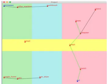
The drone is dedicated to maintaining the connection between the nodes in a smart home. For example, it is used in the scenario of sending a message from node microwave to node tv2 where a connection is missing between the two other nodes toothbrush and clock1 due to the scope of the wireless technology (Figure 3). In this case, a drone moves to retrieve the message from the toothbrush to send it to the computer node by way of the drone moving to reach messages from the microwave and its links. Then, it estimates the rank to send messages to the nearest nodes and finally passes them to the destination node tv2.
Fig. 3. A simulation scenario for passing messages between two communication nodes using a drone
V. ANALYSIS OF SIMULATIONS RESULTS
This study focused on the connectivity of IoT technologies over large areas. Because these devices are essential for rescuing people in dangerous areas, while maintaining low cost and
minimal human interaction possible. Our results suggest that it is possible to communicate in an isolated area on which the Internet and wireless connection having breakdowns or is not possible in certain sub-areas. In our last simulation case study, a drone maintains connectivity and conveys messages to the intended destination. This solution can use Lora's Lopy4 technology, for its own peer-to-peer wireless connection, by which a drone and an optimization algorithm seem to be suitable to address the problem. The same drone can also be used to send acknowledgments to the sender if needed. However, drawbacks of the drone approach include that it can encounter obstacles or function unexpectedly during rainy or windy weather.
VI. CONCLUSION AND FUTUR WORK
The smart devices have limited capabilities, energy, memory, and ranking, so their access to remote resources is crucial for maintaining the function, while reducing the response time. Solving the challenge of reaching and accessing remote resources most efficiently is important and selecting the resource with the shortest path can improve the performance of IoT devices. Comparisons of path searching algorithms in real-time allowed for observation of the advantages and faults. The primary advantage is distributing the search for a path along the course of the path and making the result less precise but saving significant time by reducing waiting. Even though the final execution time was often similar, splitting into numerous iterations of TBA* and LRTA* compared to A* makes the application more fluid and reduces delays. While the paths are less optimized, the differences are not always noticeable.
These algorithms in the current versions cannot dynamically change the topology of a distributed system. While they are powerful for traversing a fixed graph, they are not suitable for networks with connections between the nodes changing during the path search.
The selected algorithm depends on the requirements and topology of the network. For a fixed network with little change, real-time algorithms can be considered, which could be further optimized via variants using a pre-path calculation to speed the process. However, in a dynamic network that changes its structure rapidly, significant errors may occur.
Three simulation case studies have also been identified and implemented, for proof of concept. They maintain connectivity and help people in a harsh environment where the network can fail. In future work, connectivity techniques will be designed and applied, inspired by A*, to route the message using the peer-to-peer connection and IoT technologies such as Wi-Fi Direct, Wifi, and LoraWAN.
ACKNOWLEDGMENT
This work was sponsored by the University of Quebec at Chicoutimi and FUQAC, Chicoutmi (Quebec), Canada.
REFERENCES
[1] Ghassan Fadlallah, Hamid Mcheick, and Djamal Rebaine. Layered Architectural Model for Collaborative Computing in Peripheral Autonomous Networks of Mobile Devices. The 16th International Conference on Mobile Systems and Pervasive Computing Mobispc’2019,
Elsevier, vol. 155, pp. 201-209, August 19-21, 2019, Halifax, NB, Canada.
[2] A. Tanweer, “A Reliable Communication Framework and Its Use in Internet of Things (IoT),” International Journal of Scientific Research in Computer Science, Engineering and Information Technology. 2018 IJSRCSEIT, Volume 3, Issue 5, ISSN : 2456-3307.
[3] B. Durmus, O. Guneri, A. Incekirik, “Comparison of Classic and Greedy Heuristic Algorithm Results in Integer Programming: Knapsack Problems,” Mugla Journal of Science and Technology, (2019). 10.22531. [4] Cisco Networking Academy, Routing Protocols Companion Guide, ISBN
0133476308, 9780133476309, 792 pages, Cisco Press, 2014.
[5] X. Yin and J. Yang, “Shortest Paths Based Web Service Selection in Internet of Things,” Hindawi Publishing Corporation Journal of Sensors, 2014.
[6] E. Mouhcine et al., “An Internet of Things (IOT) based Smart Parking Routing System for Smart Cities,” (IJACSA) International Journal of Advanced Computer Science and Applications, Vol. 10, 2019.
[7] Jabril Abdelazizi. Architectural Model for Collaboration in The Internet of Things; A Fog Computing Based Approach, PhD Thesis, University of Quebec at Chicoutimi, 141 pages, 2018.
[8] W. Winfredruby and S. Sivagurunathan, “Data Security and Shortest Path Finding in IOT”, (IJSRCSEIT) International Journal of Scientific Research in Computer Science, Engineering and Information Technology, Vol. 5, 2019.
[9] M. el-Tager and Y Gadallah, “SWSP: Socially-Weighted Shortest Path Routing for Practical Internet of Things Applications”, (WCNC) IEEE Wireless Communications and Networking Conference, 2019.
[10] D. Z. Fawwaz, S. Chung, and H. Lee, “Dynamic IoT-Fog Task Allocation using Many-toOne Shortest Path Algorithm,” (IoTaIS) IEEE International Conference on Internet of Things and Intelligence System, 2019. [11] Chang Wook Ahn, Advances in Evolutionary Algorithms: Theory,
Design and Practice. NY, USA, Springer, 2006.
[12] Cisco Networking Academy, Routing Protocols Companion Guide, ISBN 0133476308, 9780133476309, 792 pages, Cisco Press, 2014.
[13] B. Gonen and S. J. Louis, “Genetic Algorithm Finding the Shortest Path in Networks,” International Conference on Genetic and Evolutionary Methods, 2011.
[14] J.M. Cargal. Discrete Mathematics for Neophytes, Numer Theory, Probability, Chap 9, 2013.
[15] C.W. Ahn and R.S.Ramakrishna. “A genetic algorithm for shortest path routing problem and the sizing of populations,” IEEE Transactions on Evolutionary Computation, Vol.6 , Issue: 6, Dec 2002.
[16] R. M. F. Alves and C. R. Lopes, “Solving Planning Problems with LRTA*,” In Proceedings of the 15th International Conference on Enterprise Information Systems (ICEIS-2013), pp. 475-481, 2013. [17] M. Ammar, S. Nirod, and G. Tan, “Solving shortest path problem using
particle swarm optimization,” Applied Soft Computing, Volume 8, 2008. [18] D. Sun and M. Li, “Evaluation function optimization of a-star algorithm in optimal path selection,” Rev. Téc. Ing. Univ. Zulia, 39(4)(2016) 105-111.
[19] B. Gonen and S. J. Louis, “Genetic Algorithm Finding the Shortest Path in Networks,” International Conference on Genetic and Evolutionary Methods, 2011.
[20] Alia Ghaddar, Monah Abou Hattoum, Ghassan Fadlallah and Hamid Mcheick. MCCM: An Approach for Connectivity and Coverage Maximization, Future Internet 2020, 12(2), 19; Impact factor 1.89; Special Issue: The Internet of Things for Smart Environments, Published: 21 January 2020.
[21] Elhoseny, M.; Hassanien, A.E. Expand Mobile WSN Coverage in Harsh Environments; In Dynamic Wireless Sensor Networks; Springer: Cham, Switzerland, 2019; pp. 29-52, doi:10. 1007.
[22] Sharma, D.; Gupta, V. Improving coverage and connectivity using harmony search algorithm in wireless sensor network. In Proceedings of the 2017 International Conference on Emerging Trends in Computing and Communication Technologies (ICETCCT), Dehradun, India, 17-18 November 2017; pp. 1-7, doi:10.1109, ICETCCT.2017. 8280297.