HAL Id: tel-03125685
https://tel.archives-ouvertes.fr/tel-03125685
Submitted on 29 Jan 2021HAL is a multi-disciplinary open access archive for the deposit and dissemination of sci-entific research documents, whether they are pub-lished or not. The documents may come from teaching and research institutions in France or abroad, or from public or private research centers.
L’archive ouverte pluridisciplinaire HAL, est destinée au dépôt et à la diffusion de documents scientifiques de niveau recherche, publiés ou non, émanant des établissements d’enseignement et de recherche français ou étrangers, des laboratoires publics ou privés.
expert knowledge integration for automotive effect
paints
Amélie Périssé
To cite this version:
Amélie Périssé. Color formulation algorithms improvement through expert knowledge integration for automotive effect paints. Chemical engineering. Université de Pau et des Pays de l’Adour, 2020. English. �NNT : 2020PAUU3025�. �tel-03125685�
Université de Pau et Pays de l’Adour
École doctorale Sciences Exactes et leurs Applications 211
Spécialité : ChimiePar Amélie PÉRISSÉ
C
OLOR FORMULATION ALGORITHMS IMPROVEMENT
THROUGH EXPERT KNOWLEDGE INTEGRATION
FOR AUTOMOTIVE EFFECT PAINTS
Amélioration des algorithmes de contretypage de teintes via
l’intégration de connaissances expertes pour les
peintures automobiles à effets
Thèse CIFRE avec BASF France division Coatings
Directrice de thèse
Dominique LAFON-PHAM (IMT Mines Alès)
Encadrant de thèse
Belkacem OTAZAGHINE (IMT Mines Alès)
Tuteur industriel Marion L’AOT
Université de Pau et Pays de l’Adour
Doctoral school of exact sciences and their applications 211
Specialization: ChemistryBy Amelie PERISSE
C
OLOR FORMULATION ALGORITHMS IMPROVEMENT
THROUGH EXPERT KNOWLEDGE INTEGRATION
FOR AUTOMOTIVE EFFECT PAINTS
Amélioration des algorithmes de contretypage de teintes via
l’intégration de connaissances expertes pour les
peintures automobiles à effets
CIFRE PhD thesis with BASF France division Coatings
Thesis director
Dominique LAFON-PHAM (IMT Mines Alès)
PhD supervisor
Belkacem OTAZAGHINE (IMT Mines Alès)
Industrial supervisor Marion L’AOT
Contents
CHAPTER 1.INTRODUCTION ... 1
1.1. CONTEXT ... 1
1.2. THESIS ORGANIZATION ... 3
CHAPTER 2.FROM LIGHT TO COLOR ... 7
2.1. LIGHT SOURCE ... 8
2.1.1. Visible spectrum ... 8
2.1.2. Light sources ... 9
2.1.3. Light: wave-particle duality ... 11
2.1.3.1. Quantum approach ... 11
2.1.3.2. Wave approach ... 12
2.2. LIGHT-MATTER INTERACTIONS ... 12
2.2.1. Light processes ... 13
2.2.1.1. Reflection and reflectance ... 13
2.2.1.2. Refraction ... 14
2.2.1.3. Absorption and absorbance ... 14
2.2.1.4. Interference of light ... 14
2.2.2. Scattering and diffraction ... 15
2.2.2.1. Light scattering by a particle ... 15
2.2.2.1.1. Mie theory ... 16
2.2.2.1.2. Rayleigh theory ... 16
2.2.2.2. Light scattering by a group of particles ... 17
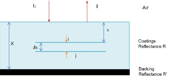
2.2.2.3. The Kubelka-Munk theory ... 18
2.3. HUMAN COLOR VISION ... 23
2.3.1. Anatomy of the eye... 23
2.3.1.1. The cornea ... 24
2.3.1.2. The iris and the pupil ... 24
2.3.1.3. The lens ... 24
2.3.1.4. The retina ... 24
2.3.1.5. The optic nerve... 25
2.3.2. Structure of the retina ... 25
2.3.2.1. Pigmented cells ... 26
2.3.2.2. Rods and cones ... 26
2.3.2.3. Bipolar cells ... 27
2.3.2.4. Horizontal cells ... 27
2.3.2.5. Ganglion cells ... 28
2.3.3. Visual phototransduction ... 28
2.3.4. The visual pathway ... 30
2.3.4.1. The optic chiasma ... 31
2.3.4.2. The lateral geniculate nucleus (LGN) ... 31
2.3.4.3. From the LGN to color perception ... 32
2.3.5. Visual adaptation to the environment ... 33
2.3.6. Human visual acuity ... 35
CHAPTER 3.COLOR MEASUREMENT ... 39
3.1. STANDARDIZATION OF LIGHT SOURCES ... 40
3.1.1. Photometry ... 40
3.1.2. CIE illuminants ... 41
3.1.2.1. CIE standard illuminants ... 41
3.1.2.2. CIE illuminants ... 42
3.2. BASIC COLORIMETRY ... 43
3.2.1. The CIE 1931 2° Standard Colorimetric Observer ... 43
3.2.1.1. RGB system ... 43
3.2.1.2. XYZ system ... 44
3.2.2. The CIE 1964 Standard Colorimetric Observer ... 46
3.3. ADVANCED COLORIMETRY ... 48
3.3.1. Noticeable color differences ... 48
3.3.1.1. Luminance differences ... 48
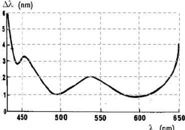
3.3.1.2. Wavelength differences ... 49
3.3.1.3. Chromaticity differences ... 50
3.3.2. Uniform color spaces ... 50
3.3.2.1. CIELab color space ... 50
3.3.2.1.1. Definition of CIELab coordinates ... 51
3.3.2.1.2. Limitations of the CIELab color space ... 53
3.3.2.2. CIECAM02 based color space... 56
3.3.3. Color differences ... 60
3.3.3.1. CIE 1976 color difference formulas ... 60
3.3.3.2. CMC (l:c) ... 61
3.3.3.3. AUDI95 ... 62
3.3.3.4. AUDI2000 or DIN6175 ... 62
3.4. CONCLUSION ... 63
CHAPTER 4.AUTOMOTIVE COATINGS ... 65
4.1. REFINISH COATINGS ... 66
4.1.1. Composition of the basecoat ... 67
4.1.1.1. Formulation of the basecoat ... 67
4.1.1.2. Tinting bases ... 68
4.1.1.2.1. Solid tinting bases ... 68
4.1.1.2.2. Effect tinting bases ... 70
4.1.1.2.2.1. Metallic pigments ... 71
4.1.1.2.2.2. Special effect pigments ... 72
4.1.1.2.3. Flop modifier ... 75
4.1.2. Sample preparation ... 75
4.2. COLOR AND TEXTURE EVALUATIONS ... 76
4.2.1. Color evaluation ... 77
4.2.1.1. Instruments measuring color ... 77
4.2.1.1.1. Spectroradiometers ... 77 4.2.1.1.2. Spectrophotometers ... 78 4.2.1.1.3. Tristimulus-filter colorimeters ... 78 4.2.1.2. Measurement geometries ... 78 4.2.2. Texture evaluation ... 80 4.2.3. Visual evaluation ... 82
4.2.4. Color and texture evaluation ... 83
CHAPTER 5.DEFINITION OF NEW TEXTURE DESCRIPTORS ... 89
5.1. IDENTIFICATION OF COMPONENTS WITH A VISIBLE INFLUENCE ON BASECOAT PERCEPTION .. 90
5.1.1. Tinting bases used and their associated effects ... 90
5.1.2. Creation of ranges ... 92
5.1.3. Analysis of the influence of four categories of tinting bases on visual appearance ... 93
5.1.4. Assessment of the different ranges ... 100
5.2. CATEGORIZATION TEST IN ORDER TO DETERMINE NEW TEXTURE DESCRIPTORS ... 101
5.2.1. Presentation of the different sorting methods ... 101
5.2.2. Procedures for the free sorting task ... 102
5.2.3. Results on the free sorting task ... 105
5.3. STANDARDIZATION OF THE WORDING USED BY BRAINSTORMING METAPLAN® ... 106
5.4. PRELIMINARY TESTS ON NEW TEXTURE DESCRIPTORS BY THREE EXPERT OBSERVERS ... 110
5.5. TEXTURE SCALE CREATION ... 115
5.6. ASSESSMENT ON THE DEFINITION OF NEW TEXTURE DESCRIPTORS ... 126
CHAPTER 6.ELABORATION OF SENSORIAL PROFILES ... 129
6.1. PROTOCOL OF EVALUATION ... 129
6.2. ELABORATION OF SENSORIAL PROFILES ... 131
6.2.1. Ratings on the descriptor Color ... 132
6.2.2. Assessments of the descriptor Contrast... 133
6.2.3. Evaluation of the descriptor Size ... 136
6.2.4. Elaboration of sensorial profile for the descriptor Intensity ... 140
6.2.5. Estimation of the descriptor Quantity ... 144
6.3. STATISTICAL ANALYSIS PERFORMED ON VISUAL ASSESSMENT DATA FOR THE DEFINITION OF THE MEAN OBSERVER ... 147
6.3.1. Outlier labelling ... 148
6.3.2. Definition of the mean observer ... 149
6.4. ASSESSMENT ON THE ELABORATION OF SENSORIAL PROFILES ... 155
CHAPTER 7.DEFINITION OF PHYSICAL TEXTURE DESCRIPTORS ... 157
7.1. PICTURE ACQUISITION ... 158
7.1.1. System of acquisition... 158
7.1.2. Calibration of the picture acquisition system ... 160
7.1.3. Presentation of the assembly and lighting systems used for picture acquisition 162 7.1.4. Picture acquisition ... 165
7.2. BASICS OF PICTURE ANALYSIS ... 167
7.2.1. Filtering operations ... 167
7.2.2. Segmentation ... 168
7.2.3. Dilation, erosion, opening and closing... 169
7.2.4. Histogram analysis and statistical measurement ... 171
7.3. PICTURE ANALYSIS FOR THE DETERMINATION OF PHYSICAL TEXTURE DESCRIPTORS ... 175
7.3.1. Selection and pretreatment of the region of interest ... 175
7.3.2. Definition of Contrast by histogram analysis ... 178
7.3.3. Determination of Size based on opening operations ... 186
7.3.4. Definition of Quantity by histogram analysis ... 192
7.3.5. Determination of Intensity based on histogram analysis ... 194
7.4. DETERMINATION OF PANEL SIMILARITIES ... 197
CHAPTER 8.CONCLUSION AND OUTLOOK ... 207
APPENDIX A. ADDITIONAL DATA ON THE ELABORATION OF SENSORIAL PROFILES ... 211
A.1. RATINGS OBTAINED ON THE DESCRIPTOR CONTRAST BY 12 OBSERVERS ... 211
A.2. RATINGS OBTAINED ON THE DESCRIPTOR SIZE BY 12 OBSERVERS ... 212
A.3. RATINGS OBTAINED ON THE DESCRIPTOR INTENSITY BY 12 OBSERVERS... 213
A.4. RATINGS OBTAINED ON THE DESCRIPTOR QUANTITY BY 10 OBSERVERS ... 214
APPENDIX B.ADDITIONAL DATA ON PICTURE ANALYSIS ... 215
B.1. STATISTICAL MEASUREMENTS FOR THE DETERMINATION OF THE DESCRIPTOR CONTRAST 215 B.2. RESULTS OF OPENING OPERATIONS FOR THE DETERMINATION OF THE DESCRIPTOR SIZE . 217 B.3. STATISTICAL MEASUREMENTS FOR THE DETERMINATION OF THE DESCRIPTOR QUANTITY . 219 B.4. STATISTICAL MEASUREMENTS FOR THE DETERMINATION OF THE DESCRIPTOR INTENSITY . 220 REFERENCES ... 221
List of figures
Figure 1-1: Launch colors of the Peugeot 208 (Yellow Faro), the Renault Clio (Orange Valencia), the Citroen C4 Cactus (Emerald Crystal) or the Audi RS Q3 Sportback (Green Kyalami) from
(Turbo, 2019) ... 1
Figure 1-2: Noticeable color differences between the aisle, the hood and the bumper after repair (Carrosserie-Geneve.Ch, 2015) ... 2
Figure 2-1: Color perception inspired from (Chrisment et al., 1994) ... 8
Figure 2-2: Electromagnetic spectrum and visible spectrum from (ChemistryLibreTexts, 2018) . 9 Figure 2-3: Colored sensations according to lighting conditions from (X-Rite, 2018c) ... 10
Figure 2-4: Electric and magnetic fields from (Tang, 2015) ... 11
Figure 2-5: Comparison of two colored cars (one blue car - in blue - and one red car - in red) inspired from (Chrisment et al., 1994) ... 13
Figure 2-6: Light reflection adapted from (Klein, 2010) ... 13
Figure 2-7: Light refraction adapted from (Klein, 2010) ... 14
Figure 2-8: Interference of light at a layer of different refractive indices from (Klein, 2010a) ... 15
Figure 2-9: Light scattering from (Bohren and Huffman, 2007) ... 15
Figure 2-10: Loss of scattering due to particle scattering volumes overlapping ... 17
Figure 2-11 : Schematic diagram of light traveling in a colorant layer inspired from (Geniet, 2013) ... 18
Figure 2-12: Anatomy of the eye from (Iristech, 2018) ... 23
Figure 2-13: Structure of the retina, picture adapted from (Salesse, 2017) ... 25
Figure 2-14: Spectral sensitivity of the S, M and L cones from (Fairchild, 2013c)... 26
Figure 2-15: Density of photoreceptors (blue for cones and black for rods) in the retina from (Fairchild, 2013c) ... 27
Figure 2-16: Rod (left) and cone (right) structures from (Powell, 2016) ... 28
Figure 2-17: Schematic of the visual phototransduction from (Leskov et al., 2000) ... 29
Figure 2-18: Conversion of all-trans-retinal to 11-cis-retinal from (Kono et al., 2008) ... 30
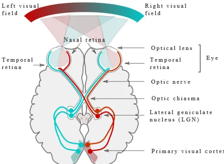
Figure 2-19: Visual pathway from the retina to the primary visual cortex from (Elster, 2018) .... 31
Figure 2-20: Schematic diagram of the left LGN from (Tovée, 2008) ... 32
Figure 2-21: Simplified color vision model diagram adapted from (Boynton, 1986) ... 33
Figure 2-22: Dark adaptation curve from (Fairchild, 2013c) where the rods take the advantage over the cones after 10 minutes before reaching their maximum of efficiency after 30 minutes ... 34
Figure 2-23: Simulation of the Purkinje shift from photopic conditions (left side) to mesopic conditions (middle) and then scotopic conditions (right side) adapted from (Wikipedia, 2019b) ... 35
Figure 2-24: Snellen eye chart for visual acuity measurement from (Lindfield and Das-Bhaumik, 2009) ... 35
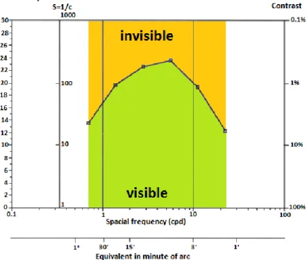
Figure 2-25: Contrast sensitivity function with the invisible part in orange and the visible part in green adapted from (Zanlonghi, 1991) ... 36 Figure 2-26: Adaptation of the trigonometric relations to determine the size of a detail in a scene ... 37 Figure 2-27: Example of simultaneous contrast from (Carbon, 2014) ... 37 Figure 2-28: Differences in color perception: A, normal trichromatic vision, B protanopia vision, C
deuteranopia vision and D tritanopia vision from (Wikipedia, 2019a) ... 38
Figure 3-1: Spectral luminous efficiency functions, V(λ) and V’(λ), defining the standard photometric observers for photopic and scotopic vision (Fotios and Goodman, 2012) ... 40 Figure 3-2: Relative spectral power distribution of the CIE standard illuminants A (in blue) and D65 (in orange) standardized to 100 at a wavelength of 560nm adapted from (Fairchild, 2013b) ... 42 Figure 3-3: Color matching functions for the CIE 1931 RGB system using monochromatic
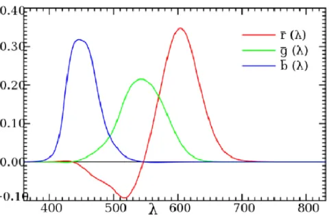
primaries at 700.0, 546.1 and 435.8 nm adapted from (Fairchild, 2013b) ... 44 Figure 3-4: Standard color matching functions for the CIE 1931 XYZ system adapted from
(Fairchild, 2013b) ... 45 Figure 3-5: The CIE xy chromaticity diagram from (Perz, 2010) ... 46 Figure 3-6: Color matching functions for the CIE 1931 XYZ system using monochromatic
primaries at 700.0, 546.1 and 435.8 nm (solid lines) and for the CIE 1964 𝑋10𝑌10𝑍10 system using monochromatic primaries 645.2, 526.3 and 444.4nm at (dotted lines) adapted from (Schanda, 2007) ... 47 Figure 3-7: Brightness, saturation and hue definitions adapted from (Perz, 2010)... 48 Figure 3-8: Left: Weber experiment on luminance differences; Right: Luminance sensitivity or
Weber curve as observed for “white” stimuli adapted from (Wyszecki and Stiles, 1982e) .. 49 Figure 3-9: Wright and Pitt experiments on wavelength differences adapted from (Wyszecki and
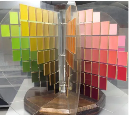
Stiles, 1982e) ... 49 Figure 3-10: MacAdam ellipses plotted in the CIE 1931 xy chromaticity diagram from (Perz, 2010) ... 50 Figure 3-11: Extension of the CIE recommendation for negative lightness values made by Pauli ... 51 Figure 3-12: CIELab color space ... 53 Figure 3-13: Munsell color tree representation with the branches representing each hue category
from (Munsell.COLOR, 2019, Larboulette, 2007) ... 54 Figure 3-14: Munsell colors of chroma and hue at value 5 plotted in the CIELab a*b* plane from
(Fairchild, 2013a) ... 55 Figure 3-15: Modeling of the conditions of observations and the different components of the
viewing field adapted from (Mornet, 2011, Luo and Li, 2007) ... 56 Figure 3-16: Schematic diagram of the CIECAM02 model adapted from (Luo and Li, 2007) .... 57 Figure 3-17: Representation of the cartesian coordinate differences between a reference (R) and
a sample (S) adapted from (Chrisment et al., 1994) ... 60 Figure 3-18: Representation of the polar coordinate differences between a reference (R) and a
Figure 4-1: Arrangement of the different layers in automotive coatings (BASF.Coatings.GmbH,
2012) ... 65
Figure 4-2: Arrangement of the different layers in refinish coatings ... 66
Figure 4-3: Proportions of the different components in the basecoat formula ... 67
Figure 4-4: Color wheel from (Hoelscher, 2018) ... 69
Figure 4-5: Relative light scattering power of rutile TiO2 for blue, red and green light as function of TiO2 particle size from (DuPontTM, 2007) ... 70
Figure 4-6: Light microscopy images of two letdowns, scale indicating 50 µm. Left: cornflake aluminum tinting base mixed with black tinting base. Right: silver dollar aluminum tinting base mixed with black tinting base ... 71
Figure 4-7: SEM picture of a cross-section through a mica-based particle with a single layer of titanium dioxide from (Pfaff, 2009) ... 73
Figure 4-8: SEM picture of a cross-section through a silica-based particle coated with α-Fe2O3 (Eivazi, 2010) ... 74
Figure 4-9: Left: SEM picture of a diffractive pigment (Pfaff, 2009); Right: SpectraFlair® multi-rainbow effects ... 74
Figure 4-10 : Orientation behavior of effect pigments in a solventborne car refinish basecoat with (top) and without (bottom) flop modifier, the scale indicates 20µm from (Maile et al., 2005) ... 75
Figure 4-11: Schematic principle of a color measuring device from (Klein, 2010b) ... 77
Figure 4-12: Directional measuring geometries: a) 45:0 and b) 0:45 from (Klein, 2010b) ... 79
Figure 4-13: Diffuse geometry d:0 adapted from (Klein, 2010b) ... 79
Figure 4-14: Principle of a multi-angle spectrophotometer from (Klein, 2010b) ... 79
Figure 4-15: Picture of Peugeot Metallic Grey (left) and Honda Vogue Silver (right) ... 81
Figure 4-16: Light microscopy observations of two commercial colors, scale indicating 50µm. Left (A): Peugeot Metallic Grey. Right (B): Honda Vogue Silver ... 81
Figure 4-17: Panel orientation under different viewing angles ... 82
Figure 4-18: Color measurement geometries for the BYK Mac (-15° is not drawn) from (BYK.Gardner.GMBH, 2009) ... 83
Figure 4-19: Texture measurement geometries for the BYK Mac from (BYK.Gardner.GMBH, 2009) ... 84
Figure 4-20: Images from BYK Mac under directional conditions (A – low sparkle & B – high sparkle) and diffuse (C – low graininess & D – high graininess) conditions from (BYK.Gardner.GMBH, 2009) ... 84
Figure 4-21: Color measurement geometries for the MA-T6 (in orange), directional texture measurement geometries (in blue) and diffuse texture measurement geometry (in red) adapted from (Ehbets et al., 2012) ... 85
Figure 4-22: Images from MA-T6 under directional (left) and diffuse (right) conditions from (X-Rite, 2018b) ... 86
Figure 5-1: Associated effects of the five categories of tinting bases ... 91 Figure 5-2: Letdowns of M99/00 with A926, from 100% to 0% of aluminum tinting base content ... 94 Figure 5-3: Sorting of letdowns with 100% of aluminum tinting base from Range 1 according to
the strength of the effect by 5 observers ... 94 Figure 5-4: Sorting of letdowns with 10% of aluminum tinting base from Range 1 according to the
strength of the effect by 5 observers ... 95 Figure 5-5: Reflectance curves of the panels from Range 2 with 0% of M99/00 (in blue), 5% of
M99/00 (in green), 50% of M99/00 (in yellow), 90% of M99/00 (in orange), 95% of M99/00 (in red) and 100% of M99/00 (in purple) ... 96 Figure 5-6: Panels from Range 2 with different percentages of aluminum tinting base, M99/00, in
green tinting base ... 96 Figure 5-7: Panels from Range 2 with different percentages of aluminum tinting base, M99/21, in
green tinting base ... 97 Figure 5-8: Light microscopy images of two letdowns: 70% M99/04 + 30% A035 (A) and 70%
M99/04 + 30% A097 (B), scale indicating 50 µm ... 97 Figure 5-9: Pictures of two letdowns 70% M99/04 + 30% A035 (A) and 70% M99/04 + 30% A097
(B) ... 98 Figure 5-10: Light microscopy images of four letdowns: 70% M99/21 + 30% A115 (A), 70%
M99/21 + 25% A115 + 5% A035 (B), 70% M99/21 + 20% A115 + 10% A035 (C) and 70% M99/21 + 5% A115 + 25% A035 (D), scale indicating 50µm ... 99 Figure 5-11: Photographs of four letdowns: 70% M99/21 + 30% A115 (A), 70% M99/21 + 25%
A115 + 5% A035 (B), 70% M99/21 + 20% A115 + 10% A035 (C) and 70% M99/21 + 5% A115 + 25% A035 (D) ... 100 Figure 5-12: Example of letdowns randomly selected for the free sorting task ... 103 Figure 5-13: Number of groups created by observers during the free sorting task, in blue for a
sorting based on texture, in yellow based on color and in green based on texture + color. The expert observers are indicated by an asterisk. ... 105 Figure 5-14: Structure of the brainstorming sessions in five phases ... 107 Figure 5-15: Word cloud of the ideas obtained during all brainstorming sessions ... 108 Figure 5-16: Reduced word cloud of the ideas obtained during all the brainstorming sessions after
gathering... 108 Figure 5-17: Sorting of 17 terms defined during brainstorming sessions into six categories of
descriptors ... 110 Figure 5-18: Image of the thirteen panels from Range A, 60% Alu + 40% A926 ... 111 Figure 5-19: Analysis of the number of groups created (min, max and mean) during the stage of
assessment by three experts on texture descriptors ... 112 Figure 5-20: Comparison of the ratings of the twins from Range G on each visual descriptor by
three observers (OBS1, OBS2 & OBS3), T1 and T2 indicated respectively Twin1 or Twin2 ... 114 Figure 5-21: Pictures of the four references created for the descriptor Size ... 116 Figure 5-22: Light microscopy image of white pearl tinting base mixed with black tinting base,
Figure 5-23: Pictures of the eight references created for the descriptor Color ... 118
Figure 5-24: Pictures of the six references for the descriptor Contrast ... 119
Figure 5-25: Pictures of the four references used for the range Intensity ... 120
Figure 5-26: Pictures of the twelve references created for the range Quantity ... 122
Figure 5-27: Analysis of the popularity of the twelve propositions of references developed for the descriptor Quantity according to the selection done by the observers ... 123
Figure 5-28: Light microscopy observations of the ChromaFlair® Red/Gold 000 (left side, picture A) and Silver/Green 060 (right side, picture B), scale indicated 50 µm ... 123
Figure 5-29: Pictures of the six references proposed for the descriptor Face-Flop ... 124
Figure 5-30: Example of a panel holder for the visual evaluation of contrast with standards #1 and #2 also called Contrast_Inexistent (K_1) and Contrast_Very Low (K_2) ... 125
Figure 5-31: Panel holder used for Color evaluation with the eight standards (where #1 = C_1 - Color_Gold, #2 = C_2 – Color_Orange , #3 = C_3 – Color_Red, #4 = C_4 – Color_White, #5 = C_5 – Color_Green, #6 = C_6 – Color_Blue, #7 = C_7 – Color_Violet and #8 = C_8 – Color_Aluminum) ... 126
Figure 6-1: Answer sheet of one observer for the evaluation of the descriptor Size ... 131
Figure 6-2: Organization of the elements in the light booth for the evaluation of the size where three panel holders are installed, one of which being placed on the rotating system ... 132
Figure 6-3: Evaluation made by 12 observers under diffuse lighting conditions on the descriptor Contrast for 34 panels, where panels K_1 to K_6 are the standards of the range Contrast ... 134
Figure 6-4: Evaluation made by 12 observers under diffuse lighting conditions on the descriptor Contrast for the panels of the range Contrast ... 135
Figure 6-5: Evaluation made by 12 observers under diffuse lighting conditions on the descriptor Contrast for the panels of the range Quantity ... 135
Figure 6-6: Evaluation made by 12 observers under diffuse lighting conditions on the descriptor Contrast for the panels of the range Color ... 136
Figure 6-7: Evaluation made by 12 observers under diffuse lighting conditions on the descriptor Size for 34 panels, where panels S_1 to S_4 are the standards of the range Size ... 137
Figure 6-8: Evaluation made by 12 observers under diffuse lighting conditions on the descriptor Size for the panels of the range Size ... 138
Figure 6-9: Evaluation made by 12 observers under diffuse lighting conditions on the descriptor Size for the panels of the range Intensity... 138
Figure 6-10: Evaluation made by 12 observers under diffuse lighting conditions on the descriptor Size for the panels of the range Quantity... 139
Figure 6-11: Evaluation made by 12 observers under diffuse lighting conditions on the descriptor Size for the panels of the range Color ... 139
Figure 6-12: Evaluation made by 12 observers under diffuse lighting conditions on the descriptor Size for the panels of the range Contrast ... 140
Figure 6-13: Evaluation made by 12 observers under directional lighting conditions on the descriptor Intensity for 34 panels where panels I_1 to I_4 are the standards of the range Intensity ... 141
Figure 6-14: Evaluation made by 12 observers under directional lighting conditions on the descriptor Intensity for the panels of the range Intensity ... 142 Figure 6-15: Evaluation made by 12 observers under directional lighting conditions on the
descriptor Intensity for the panels of the range Size ... 142 Figure 6-16: Evaluation made by 12 observers under directional lighting conditions on the
descriptor Intensity for the panels of the range Contrast ... 143 Figure 6-17: Evaluation made by 12 observers under directional lighting conditions on the
descriptor Intensity for the panels of the range Color ... 143 Figure 6-18: Evaluation made by 12 observers under directional lighting conditions on the
descriptor Intensity for the panels of the range Quantity ... 144 Figure 6-19: Evaluation made by 10 observers under diffuse lighting conditions on the descriptor
Quantity for 34 panels where panels from Q_1 to Q_12 are the propositions of the range Quantity and the references are indicated with asterisk ... 145 Figure 6-20: Evaluation made by 10 observers under diffuse lighting conditions on the descriptor
Quantity for the panels of the range Quantity ... 146 Figure 6-21: Evaluation made by 10 observers under diffuse lighting conditions on the descriptor
Quantity for the panels of the range Color ... 146 Figure 6-22: Evaluation made by 10 observers under diffuse lighting conditions on the descriptor
Quantity for the panels of the range Contrast ... 147 Figure 6-23: Probability plot obtained after normality test in Minitab for the ratings of panel K_2 ... 150 Figure 6-24: Box plot obtained after the use of the Kruskal Wallis test for the evaluation of the
descriptor Contrast where the red cross indicates the mean and the blue cross or point the outliers ... 152 Figure 6-25: Number of outliers per descriptor and per observer ... 153
Figure 7-1: Impact of the ISO value on the brightness of the picture from (Mansurov, 2010a) 159 Figure 7-2: Impact of the lens aperture on the brightness and the blurry background of the picture
adapted from (Mansurov, 2010c) ... 159 Figure 7-3: How image brightness changes with the exposure time from (Mansurov, 2010b) . 160 Figure 7-4: X-Rite ColorChecker® Classic from (X-Rite, 2018a) ... 162 Figure 7-5: Spectral power distribution of one Solux incandescent lamp (36°, 12V, 50W, 4 700K)
measured with a Konica-Minolta CS-2000 spectroradiometer with a 1-degree angle ... 163 Figure 7-6: Schematic arrangement of the system used to create diffuse lighting conditions .. 164 Figure 7-7: Schematic arrangement of the system used for direct lighting conditions ... 165 Figure 7-8: Evolution of the exposure time in dependence of the lightness value L*(45°) for the 34
standard panels created for the texture scale ... 166 Figure 7-9: Example of a two-class segmentation based on pixel intensity: (a) original picture; (b)
binary picture with a threshold value of 150 from (Dupas, 2009) ... 168 Figure 7-10: Example of vicinity pixels with the 4-connected and 8-connected pixels ... 169 Figure 7-11: (a) Original image where the foreground is in white and the background in black; (b)
element; (c) eroded image where the grey pixels are the result of the erosion with a 3x3-square structuring element from (Couka, 2015) ... 170 Figure 7-12: (a) Original image where the foreground is in white and the background in black; (b)
opened image where the grey pixels are the result of the opening with a 3x3-square structuring element; (c) closed image where the grey pixels are the result of the closing with a 3x3-square structuring element from (Couka, 2015) ... 170 Figure 7-13: Procedure for the size determination by successive openings from (Maintz, 2005) ... 171 Figure 7-14: Flight display panel (left) and its associated histogram (right) from (Marques, 2011) ... 171 Figure 7-15: Example of the probability distribution according to the skewness value based on the
mean, the median et the mode values from (Jain, 2018) ... 173 Figure 7-16: Example of the shape of the histogram according to the kurtosis value from (Jain,
2018) ... 174 Figure 7-17: Histogram based pictures coming from MA-T6 measurements for three references
from the range Contrast: K_2, K_4 and K_6 ... 174 Figure 7-18: Non-uniformity of the lighting conditions explained by a photography of the panel
K_5 taken with the Nikon D800, ISO 800, f/6.3 and an exposure time of 1/2s for directional lighting. The green arrow indicates the crinkle and the red cross the center of the lighted circle. ... 176 Figure 7-19: (a) initial ROI of K_5 under directional lighting (b) resulting ROI after alternate
opening-closing filtering operations with a square of size 3 (c) resulting ROI after lighting correction ... 177 Figure 7-20: Determination of the contrast sensitivity of the visible effect particles in a panel
photographed at a distance of 70 cm for an estimated optical behavior of one particle of 6 pixels or 20 in spatial frequency, picture adapted from (Yssaad-Fesselier, 2001) ... 178 Figure 7-21: Number of pixels greater than 1.5 times the minimum value against the mean
observer for Contrast where the 6 standards of this range are identified by a bigger circle ... 179 Figure 7-22: Histograms of the Y pictures under diffuse lighting conditions for the six references
of the range Contrast ... 180 Figure 7-23: Number of pixels greater than 1.29 times the mode value against the mean observer
for Contrast where the 6 standards of this range are identified by a bigger circle ... 181 Figure 7-24: Contrast coefficient, C, against the mean observer for Contrast where the 6
standards of this range are identified by a bigger circle ... 182 Figure 7-25: Contrast coefficient, C, against the mean observer for Contrast where the 6
standards of this range are identified by a bigger circle and with the withdrawal of C_3, C_4, C_5, C_7 and I_4 due to undersaturation ... 183 Figure 7-26: Evolution of the contrast coefficient, C, on a simple and theoretical case ... 184 Figure 7-27: Evolution of the new contrast coefficient, C', on a simple and theoretical case ... 185 Figure 7-28: New contrast coefficient, C’, against the mean observer for Contrast where the 6
standards of this range are identified by a bigger circle and with the exclusion of C_3, C_4, C_5, C_7, K_2, and I_4 due to incorrect exposure time and the two solid colors K_1 and Q_1 ... 186
Figure 7-29: (a) Initial ROI of K_5 under diffuse lighting (b) Mask obtained after thresholding at 0.61 (1.29MODE) (c) Resulting masked image after removing the groups of pixels at the boundaries of the ROI ... 187 Figure 7-30: (a) Resulting mask after an opening of size 2 on K_5 (b) Resulting mask after an
opening of size 3 on K_5 (c) Resulting mask after an opening of size 4 on K_5 ... 188 Figure 7-31: Granulometric curves obtained by successive opening filtering operations with a
squared structuring element from size 2 to 10 ... 189 Figure 7-32: Slope of the granulometric curves obtained for a size 2 squared opening against the
mean observer for the descriptor Size where the 4 standards of this range are identified by a bigger circle ... 190 Figure 7-33: Size coefficient, S, against the mean observer for the descriptor Size where the 4
standards of this range are identified by a bigger circle ... 191 Figure 7-34: Size coefficient, S, against the mean observer for Size where the 4 standards of this
range are identified by a bigger circle and with the withdrawal of 2 panels due to undersaturation C_7 and I_4 ... 191 Figure 7-35: Number of pixels greater than 1.29 times the mode value against the mean observer
for Quantity where the 12 panels created for this range are identified by a bigger circle .. 192 Figure 7-36: Quantity coefficient, Q, against the mean observer for the descriptor Quantity where
the 12 standards of this range are identified by a bigger circle ... 193 Figure 7-37: Histograms of the Y pictures under direct illumination conditions for the four
references of the range Intensity ... 194 Figure 7-38: Intensity coefficient, I, against the mean observer for the descriptor Intensity where
the 4 standards of this range are identified by a bigger circle ... 196 Figure 7-39: Intensity coefficient, I, against the mean observer for the descriptor Intensity where
the 4 standards of this range are identified by a bigger circle and with the withdrawal of 5 panels due to undersaturation C_3, C_4, C_5, C_6 and I_4 ... 197 Figure 7-40: Illustrated geometric steps realized by PCA where the two axis of the initial plot (a)
are changed for principal components (b) and then rotated (c) to better illustrate a link between the number of letters of the word and the number of lines of the definition from (Abdi and Williams, 2010) ... 198 Figure 7-41: Plot of the eigenvalues for the PCA performed on the mean observer values ... 199 Figure 7-42: Biplot of individuals and variables obtained by PCA performed on the mean observer
values ... 199 Figure 7-43: Cluster dendrogram obtained by HCPC defined by PCA on the mean observer values ... 200 Figure 7-44: Cluster plot in five groups obtained by HCPC defined by PCA on mean observer
values ... 201 Figure 7-45: Radar charts of each cluster determined by PCA and HCPC based on the normalized
List of tables
Table 2-1: Several types of light sources adapted from (Klein, 2010a) ... 9
Table 3-1: Tristimulus values for some illuminants (XN, YN and ZN) for 1931 CIE 2° standard colorimetric observer or CIE 1964 10° standard colorimetric observer ... 51
Table 3-2: Parameters of viewing state of CIECAM02 from (Luo and Li, 2007) ... 57
Table 3-3: Calculation of the color appearance attributes for CIECAM02 ... 59
Table 4-1: Spectral range of absorption, light color and complementary color ... 69
Table 4-2: Comparison of optical properties between cornflake and silver dollar aluminums, from (Klein, 2010a) ... 72
Table 4-3: Color formula of aluminum grey from PSA ... 76
Table 4-4: Lightness and FI values for Peugeot Metallic Grey and Honda Vogue Silver ... 81
Table 5-1: Characteristics of the aluminum tinting bases of Line 90 ... 90
Table 5-2: Characteristics of the three white tinting bases of Line 90 ... 91
Table 5-3: Summary of the different formulations sprayed for Range 3 ... 93
Table 5-4: List of the 49 letdowns randomly selected for the free sorting task ... 104
Table 5-5: List of features used to gather the forty-nine panels during the free sorting task ... 106
Table 5-6: Global lexicon with parameter, scale and definition obtained after the brainstorming sessions with overall 70 participants ... 109
Table 5-7: Formulas prepared for the preliminary tests on new texture descriptors ... 111
Table 5-8: Results of the assessment of the three experts on texture descriptors ... 113
Table 5-9: Standardization of the conditions of observation (light source and angle) for visual assessment ... 115
Table 5-10: Description of the four references developed for the descriptor Size ... 116
Table 5-11: Description of the eight references developed for the descriptor Color ... 117
Table 5-12: Description of the six references developed for the descriptor Contrast ... 119
Table 5-13: Description of the four references developed for the descriptor Intensity ... 120
Table 5-14: Description of the twelve propositions of references for the descriptor Quantity .. 121
Table 5-15: Description of the six references developed for the descriptor Face-Flop ... 124
Table 6-1: Evaluations made by the 6 observers from the French color lab on the descriptor Color for 13 panels under directional lighting conditions ... 132
Table 6-2: Critical value for the Grubbs test with a significance level of 0.05% or 0.10% ... 148
Table 6-3: Statistical measurements for panel K_2 obtained for the descriptor Quantity ... 150
Table 6-4: Comparison of different methods for outlier detection in the ratings obtained for panel K_2 for the descriptor Quantity based on the observations of 10 participants ... 151
Table 6-5: Values of the mean observer for the four descriptors, determined after exclusion of outliers ... 154
Table 7-1: Setting of the camera Nikon D800 for picture acquisition ... 160 Table 7-2: Summary of the exposure time for picture acquisition with Nikon D800, ISO 800 and
f/6.3 for diffuse lighting conditions ... 166 Table 7-3: Sign of the skewness value according to the mean, median and mode values ... 173 Table 7-4: Exposure time selected for diffuse and directional lighting conditions for the 34
standards from texture scale ... 175 Table 7-5: Statistical characteristics inherent to the Y pictures of the panels of the range Intensity
acquired under direct conditions ... 195 Table 7-6: Quality of projections of the descriptors on the two axes ... 199 Table 7-7: Characteristics of each cluster according to the projection of the four descriptors based
on mean observer values ... 201 Table 7-8: Values of the four coefficients (C, S, Q and I) obtained by picture analysis ... 202
List of abbreviations
CAM Color appearance model CCT Correlated color temperature
CIE Commission internationale de l'éclairage (International commission on illumination
CPD Cycle per degree CT Color temperature DOI Distinctiveness of image FI Flop index
HCPC Hierarchical clustering on principal components IQR Interquartile range
IR Infrared
LED Light emitting diode LGN Lateral geniculate nucleus MAD Median absolute deviation OEM Original equipment manufacturer PCA Principal component analysis RI Refractive index
SEM Scanning electron microscopy UV Ultraviolet
Glossary
Basecoat – Colored layer used to provide the aesthetic aspect of a vehicle. Can be solid or effectBlending – Repair technique used to smoothen color differences between two adjacent elements
Bracketing – Technique used in photography to take several pictures of the same scene by using different camera settings
Clearcoat – Uncolored layer used to protect paint from environmental and chemical stresses. Can be glossy, satiny, matte or textured
Color travel – Color change according to the angle of observation Colormatching – Process of reproducing original OEM colors
Cornflake aluminum – Aluminum particles with irregular surfaces and rough edges
Edge to edge – Repair technique used when there is no difference in color between two adjacent elements
Effect color – Basecoat formulation with effect particles
Effect particles – Particles used in effect tinting bases to provide texture. Can be aluminum, interference or pearlescent.
Face view – Viewing angle of 45° compared to the normal angle Flip view – Viewing angle of 15° to 25° compared to the normal angle Flip-flop effect – Lightness change according to the angle of observation
Flop modifier – Silica microspheres which cause a disorientation of the effect particles in the coating film
Flop view – Viewing angle of 75° to 110° compared to the normal angle
Frost effect – Yellowish-gold impression at face view and bluish color impression at flop view Glass flakes – Transparent effect particles acting like little mirrors and offering an intense sparkling
Graininess – Uniformity of light-dark areas in an effect color linked to the use of effect particles
Hue extinction – When mixed with colored pigments, ability for aluminum particles to entirely hide the chroma.
ISO – Settings of the camera used to brighten or darken a picture Lens aperture – Settings of the camera used to sharpen or blur a picture Letdown – Mix of tinting bases at different percentages
Midcoat – Optional layer added between the basecoat and the clearcoat to obtain deep and vibrant colors
Mode value – Intensity value with the most occurrences in a picture histogram
Shutter time – Settings of the camera used to control the global brightness of a picture Silver dollar aluminum – Aluminum particles with plane surfaces and round edges Solid color – Basecoat formulation without effect particles
Sparkling – Distinction of flakes by the human eye due to a highly intense light reflection Specular angle – Angle of observation where the maximum of reflection is obtained
Spot repair – Repair technique used to paint a small durst without being able to distinguish a color difference
Texture – Heterogeneity of the optical film behavior linked to the use of effect particles creating local optical effects
Tinting base – Suspension of a single pigment in a matrix used in the basecoat formulation. Can be solid or effect
Chapter 1. Introduction
Contents
1.1. CONTEXT ... 1 1.2. THESIS ORGANIZATION ... 3
In various artistic or industrial sectors such as cosmetics, transports or luxury, the visual aspect of materials holds a special place. It has become a criterion of evaluation and appreciation in purchase decisions. Indeed, when buying a vehicle, the consumer selects first the brand and model of his future vehicle, then its color before selecting the technical and ergonomic characteristics. Color is a major quality factor and manufacturers need to be imaginative and original in the conception of new color trends for automobiles. This market is then governed by appearance and effects. Customers want to distinguish themselves with a good balance between color and gloss. The coatings revolution has started to fit to the customer’s needs: deep and vibrant colors with effects. The color has become so important that even the bumper is now painted. The manufacturers have been able to adapt quickly by offering bright colors from the launch of new vehicles such as the Peugeot 208 (Yellow Faro), the Renault Clio (Orange Valencia), the Citroen C4 Cactus (Emerald Crystal) or the Audi RS Q3 Sportback (Green Kyalami) presented in Figure 1-1.
Figure 1-1: Launch colors of the Peugeot 208 (Yellow Faro), the Renault Clio (Orange Valencia), the Citroen C4 Cactus (Emerald Crystal) or the Audi RS Q3 Sportback (Green Kyalami) from (Turbo, 2019)
1.1. Context
This thesis is conducted in the context of automotive paints with a special focus on refinish automotive coatings. Whatever the reason, accident or resale, a vehicle might need a repair which will involve a repainting of a specific element. In the automotive refinish area, a perfect car repair must be undetectable and invisible for the customer. According to the
quality of the color formula, different repair techniques exist. The first one is the spot repair when the quality of the color formula is close to perfection, so the initial color and the matched one look exactly the same. This quality of formula can be used to fix for example a burst of paint on the body linked to a violent door knock. With this quality, the body shop is able to repair only the burst – any difference to the rest of the element is invisible. If the area to be repaired is bigger, the element needs to be changed before being painted. If the quality of the color formula provided is acceptable, the element, for example the aisle, is dismantled, changed, painted and then reinstalled. In the final result, the observer will not be able to distinguish any difference between the aisle, the door and the hood. This type of repair is called edge to edge. Finally, when one can notice a color difference between the original color and the proposed formula without being able to improve the quality, the body shop fixes the element before reinstalling and painting it. To smoothen the color differences, the paint is sprayed also on the adjacent elements. This last technique is called “blending”; it helps to reduce color differences like those presented in Figure 1-2 where the bumper is not properly matched in color with the aisle and the hood.
Figure 1-2: Noticeable color differences between the aisle, the hood and the bumper after repair (Carrosserie-Geneve.Ch, 2015)
Customers might think that it is easy to reproduce the color of a car but in fact it requires a lot of experiments. Many years of training are required to learn how to color match. That is why, beyond the paint itself, paint manufacturers such as BASF supply to their customers color formulations which allow to reproduce each color shade of the automotive fleet namely several hundreds of thousands of colors. For each color, the formula consists of a mixture of different ingredients which, mixed together, provide a paint with a correct or at least a best possible color match. Two automotive paint categories exist: solid and effect colors. Solid colors are based on the mix of several primary colors. For effect colors, metallic or pearlescent, on top of the primary colors mix, effect particles are added to provide certain optical properties. Depending on the angle of view, the interactions between light and matter produce different effects. The particles added in the paint film produce local optical effects depending on the angle of view. These effects could modify the lightness and/or the hue of the color itself. They are responsible for the heterogeneity of the optical film behavior and therefore the effect (texturing).
Color formulas are developed in the lab by using proprietary matching software which integrates statistical and physical optical models. These models are used to estimate the resulting color starting from a formula or reflectance curves coming from spectrophotometer measurements. They are combined into algorithms which minimize the theoretical color difference between a standard and the resulting formula. However, the prediction models have their own limitations – this applies in particular to the color descriptors currently used. The colorimetric description does not allow a complete representation of the visual color perception. The color descriptors commonly used, CIELab coordinates, are quite efficient for solid colors but not efficient enough for effect colors. Indeed, visual texture descriptors are not available today to correctly characterize these effect colors and the global appearance is hence not perfectly described. The result obtained during the formulation process is not precise enough to obtain a good match after the first trial. It must be repeated several times by an experienced colorist who manually adjusts the formula to lead to a satisfying formula. Based on his own experience, the colorist is able to reproduce a color. It is also important to note that the issues of efficiency and repeatability depend on the human factor. The improvement of descriptors by the addition of texture descriptors to color descriptors would allow the enhancement of the color matching process.
The main objective of the present thesis is to qualify and to quantify the visually perceived attributes such as the sparkling effect or the size of the effect particles in the formula. In effect coatings, the sparkling effect is linked to optical manifestations at the microscopic and macroscopic levels. Effect particles are micrometric flakes which provide light interaction. In the case of aluminum particles, when they are lighted, the specular light intensity is much stronger than the incident light. These particles act like tiny mirrors and are responsible for the sparkling effect. Therefore, due to the light spreading triggered by light reflection, the sparkles could appear larger than the physical size of the particles. Besides, it is also important to consider the complexity of what is perceived by a human observer – the visual impression is based on a complex combination of color, effect particles and also the concentration of the different elements in the formula.
1.2. Thesis organization
This thesis results from a collaboration between the Center of Materials Research (C2MA) of the IMT Mines Alès and BASF France division Coatings within the framework of the CIFRE convention (Conventions Industrielles de Formation par la REcherche). The objectives of this PhD thesis are multiple. In a first step, it is necessary to define new descriptors considering the texturing of the optical signal before correlating them to the visual acceptance of a color formulation by experienced colorists. One field of investigation is based on the integration of the human color evaluation through sensorial analysis. The second axis is to adapt the perceived descriptors into physical descriptors extracted from optical data acquisitions.
At first, through the second chapter, the mechanism allowing the transformation of light into color will be presented. Color vision rests on the triplet light-object-observer and the three pillars will be discussed in detail. First, the light radiation as a combination of waves will be explained as well as different light sources. Then, the interaction of light and matter will be analyzed by considering different processes such as reflection, absorption or scattering.
Finally, it will be necessary to understand the color vision mechanism of the human visual system by considering the eye and especially the retina which plays a crucial role in color vision with its two kind of photoreceptors: cones and rods. The visual path will then be analyzed to understand the interactions between the eye and the brain. The adaptation of the human visual system to its environment and in particular to contrast and visual acuity will be explained.
The third chapter will be devoted to color measurement. To this end, first, standardization of light sources with the establishment of illuminants and the photometric methods used will be presented. Then, in order to measure color, the functioning of the human visual system was standardized by quantifying the spectral responses of its photoreceptors. This standardization led to the introduction of the two CIE standard colorimetric observers in 1931 and 1964, respectively. Colorimetry is the science of color measurement. Through the establishment of uniform color spaces such as CIELab or CIECAM02, it is then possible to define color differences to better understand the different types of color shifts. Numerous computational models have been developed to better represent the color differences distinguishable by the human visual system. A non-exhaustive list will be presented such as CIE1976, CMC (l:c), AUDI95 and AUDI2000.
The fourth chapter will focus on refinish automotive coatings. After understanding the behavior of light and matter in Chapter 2, we will herein discuss different types of pigments involved in the formulation of automotive paints such as aluminum, specific effect pigments or traditional pigments. A quick presentation of sample preparation and spraying will be made. In a second part, the state of the art considering various types of evaluations of the color is presented, instrumental as well as visual. Measuring devices such as spectroradiometers and spectrophotometers as well as the importance of the measurement angles will be detailed. For a decade, new portable devices have been introduced into the market. They allow color measurement as well as image acquisition. From the images captured by those devices, texture parameters have been derived: sparkling and graininess. However, neither of them corresponds exactly to visual appearance and perception.
After having defined the constraints and limits of the systems of measurement and the representation of color perception generated by effect colors, the fifth chapter focuses on the definition of new texture parameters. To this end, different constituents involved in the formulation of effect colors will be analyzed to better understand their impact on visual appearance. One of the objectives of the PhD thesis is to make use of expert knowledge in terms of visual expertise. The aim here is to bring these fields of expertise together and to more clearly define their respective content to better understand them and to base the new texture descriptors on what the human eye can discern and not the other way around. The different steps leading to their determination will be detailed.
The identification of texture descriptors was the first step of the expert knowledge mobilization. The aim of this sixth part is to set up sensory analysis sessions in which experienced observers will have to evaluate the different descriptors previously defined. The evaluation protocol will be detailed because it is the key to guarantee consistent ratings
between the different judges. Indeed, by standardizing the observation conditions including inclination angles and type of lighting, it is thus possible to ensure homogeneous conditions from one observer to another. Finally, in order to define the mean observer on each descriptor, different statistical data analysis methods will be presented to choose the best fitting one compared to the results obtained.
Last, but not least, the adaptation of texture descriptors into physical texture descriptors is described. For this, different samples are photographed with a high-resolution camera. At first, it is necessary to select the appropriate settings. As a matter of fact, the sensors of the device are not able to measure a large dynamic range in luminance. It is hence necessary to be able to simplify the settings during the acquisition in order to better reproduce the perception by the human visual system. Indeed, the objective is not just to measure but to measure in the way that would best fit the perception of the human eye. By setting up all the parameters except the exposure time, it will then be possible to establish a link between the luminance of the samples and the exposure time for the picture acquisition. In addition, the challenge of this part is also to reproduce the observation conditions during sensory analysis tests to be able to define a correlation between the visible and the measurable. Finally, once the lighting conditions and the settings are defined, the physical texture descriptors will be determined from the images. Statements given by expert observers will be at the origin of their definition. This should allow a better correlation between measurable and perceptible factors. Indeed, all the core of present thesis rests on the definition of texture descriptors corresponding as much as possible to the evaluations made by experts.
Finally, the results obtained during this thesis are discussed and an outlook for a potential future work in this field is given.
Chapter 2. From light to color
Contents
2.1. LIGHT SOURCE ... 8 2.1.1. Visible spectrum ... 8 2.1.2. Light sources ... 9 2.1.3. Light: wave-particle duality ... 11
2.1.3.1. Quantum approach ... 11 2.1.3.2. Wave approach ... 12
2.2. LIGHT-MATTER INTERACTIONS ... 12 2.2.1. Light processes ... 13
2.2.1.1. Reflection and reflectance ... 13 2.2.1.2. Refraction ... 14 2.2.1.3. Absorption and absorbance ... 14 2.2.1.4. Interference of light ... 14
2.2.2. Scattering and diffraction ... 15
2.2.2.1. Light scattering by a particle ... 15 2.2.2.1.1. Mie theory ... 16 2.2.2.1.2. Rayleigh theory ... 16 2.2.2.2. Light scattering by a group of particles ... 17 2.2.2.3. The Kubelka-Munk theory ... 18
2.3. HUMAN COLOR VISION ... 23 2.3.1. Anatomy of the eye... 23
2.3.1.1. The cornea ... 24 2.3.1.2. The iris and the pupil ... 24 2.3.1.3. The lens ... 24 2.3.1.4. The retina ... 24 2.3.1.5. The optic nerve... 25
2.3.2. Structure of the retina ... 25
2.3.2.1. Pigmented cells ... 26 2.3.2.2. Rods and cones ... 26 2.3.2.3. Bipolar cells ... 27 2.3.2.4. Horizontal cells ... 27 2.3.2.5. Ganglion cells ... 28
2.3.3. Visual phototransduction ... 28 2.3.4. The visual pathway ... 30
2.3.4.1. The optic chiasma ... 31 2.3.4.2. The lateral geniculate nucleus (LGN) ... 31 2.3.4.3. From the LGN to color perception ... 32
2.3.5. Visual adaptation to the environment ... 33 2.3.6. Human visual acuity ... 35 2.4. CONCLUSION ... 37
We live in a world full of light and colors. In our environment (plants, objects …), everything seems to be colored but it is important to really understand what the nature of color is. Indeed, the perception of color is a very specific field which mixes physical laws and very specific physiological and psychological conditions. This chapter will be focused on the understanding of color and its creation.
Human beings tried to understand this complex process for ages, but it is only at the end of the 17th century that they started to solve it. In 1666, Newton discovered the decomposition of sunlight when crossing a prism (Newton, 1671). For different angles, the prism refracts diverse colors, from violet to red with all shades of blue, green, yellow and orange. By this experiment, Newton showed that color is intrinsic to light.
Color perception involves several factors. First, color cannot exist without light. The light source is the first step in color sensation of the observed object. The material which constitutes the observed object reflects or transmits all or a part of the light rays (also called colored stimulus) emitted by the light source. The eyes, altogether, then capture those light rays and convert the multiple received stimulus signals into a color signal which can be transmitted to the brain. The brain will then identify and name the color of the observed object. Color perception is then highly dependent on the light source, the observed object, the eyes and the brain. The first three elements form the triplet “light-object-eye”.
Figure 2-1: Color perception inspired from (Chrisment et al., 1994)
2.1. Light source
2.1.1. Visible spectrum
Light is one of the mandatory elements for color perception. Without light, the human visual system is unable to function and consequently see colors. Light can be defined as a physical phenomenon which transports energy from one place to another in the form of electromagnetic radiation. This can also be described as a stream of photons. Photons are massless particles with a velocity equivalent to speed of light in vacuum, 299 792 458 m/s. An electromagnetic radiation is defined by its wavelength, λ in m. Even if the electromagnetic spectrum covers a wide range of wavelengths, from 10-16 m to 106 m, the visible range for the human eye is between 380 nm and 780 nm (see Figure 2-2).
The visible spectrum is continuous with no boundaries or gaps from one color to another one. Six named color ranges can be defined from this spectrum: violet (380 nm – 450 nm), blue (450 nm – 495 nm), green (495 nm – 570 nm), yellow (570 nm – 590 nm), orange (590 nm – 620 nm) and red (620 nm – 780 nm). At the boundaries of a color range, for example
at 495 nm, the color defined can be considered as a green or a blue according to the observer. By moving a little around the boundary, a greenish blue or a bluish green is then obtained, the famous turquoise.
Figure 2-2: Electromagnetic spectrum and visible spectrum from (ChemistryLibreTexts, 2018)
The visible spectrum can also be obtained when a beam of sunlight is crossing a glass prism. Newton discovered this phenomenon in 1666 and reported it in his “New Theory about Light and Colours” to the Royal Society (Newton, 1671). The conclusion drawn is that “light itself is a heterogeneous mixture of differently refrangible rays” or in other words, color is an intrinsic property of white light.
2.1.2. Light sources
Sunlight is obviously not the only existing light source. Light can be naturally or artificially produced by for example the sun, stars, fire, incandescent or fluorescent lamps or light emitting diodes (LEDs). Two types of light sources exist: temperature and luminescence radiators. They can be classified into two categories according to the way the light is obtained, naturally or artificially (Klein, 2010a). The visual reference is the sun.
Table 2-1: Several types of light sources adapted from (Klein, 2010a)
Temperature radiators Luminescence radiators
Natural Artificial Artificial
Sunlight Stars Blackbody radiator Incandescent lamp Fluorescent lamp LED
There is no equienergetic light, meaning there is no light having a continuous and flat spectrum, hence the interest of using blackbody radiators as references. To characterize the light sources, their spectral power distributions are compared with the spectral energy distribution of a blackbody radiator. At room temperature, a blackbody appears black. During its heating, a blackbody becomes red, yellow, white and then blue according to the temperature. The Planck law of radiation (2-1) gives the spectral power distribution of a blackbody radiator.
𝑆(𝜆, 𝑇)𝑑𝜆 = 2𝜋ℎ𝑐 2 (exp [ℎ𝑐
𝑘𝜆𝑇] − 1)𝜆5
𝑑𝜆 (2-1)
With S(λ, T), spectral power distribution (unit: W/m3)
λ, wavelength (unit: m) T, temperature (unit: K)
c, speed of light in vacuum (c=299 792 458 m/s) h, Planck constant (h=6.626 077 x 10-34 J.s) k, Boltzmann constant (k=1.380 648 x 10-26 J/K)
The color of the spectrum emitted by a blackbody changes with temperature; Kelvin defined a method to characterize temperature radiators: the correlated color temperature (or CCT) (Wyszecki and Stiles, 1982d). The light emitted by a radiator is compared to the temperature of the blackbody radiator which emits the maximum of light at the same color. According to the CIE1 (Commission Internationale de l’Éclairage), “the correlated color
temperature is the temperature of the Planckian radiator whose perceived color most closely resembles that of a given stimulus at the same brightness and under specified viewing conditions” (CIE, 1987).
The main natural light source is the sunlight, which is obviously not constant. The spectrum of sunlight can be associated to a black-body around 5 500 K. Known as artificial light source, lamps are electric lights and depend on the light bulb used. An incandescent light bulb is made from a tungsten wire filament which is heated by an electric current and then glows. Its CCT is around 2 800 K. This system can be compared to a black-body as its emission spectrum is only dependent on its temperature. For a halogen lamp, the filament is surrounded by a small amount of halogen gas (iodine or bromine). This combination improves the lifespan of the source and raises the color temperature to 3 100 K (Klein, 2010a). All light sources are subject to variations for several reasons. For sunlight, latitude, season, air pollution or weather conditions have a considerable impact while lifespan or materials have one for lamps. Besides, a colored sample can produce different colored sensations merely based on lighting conditions (see Figure 2-3).
Figure 2-3: Colored sensations according to lighting conditions from (X-Rite, 2018c)
1CIE : Commission Internationale de l’Éclairage which oversees normalization and standardization for
2.1.3. Light: wave-particle duality
Light is an electromagnetic wave, meaning a combination of an electric wave and a magnetic wave. The electromagnetic wave is described by two vectors: 𝐸⃗ for the electric field and 𝐵⃗ for the magnetic field (see Figure 2-4).
Figure 2-4: Electric and magnetic fields from (Tang, 2015)
2.1.3.1. Quantum approach
Light is both, a wave and a stream of particles (photons, which are massless particles). Their energy E can be described by the Planck-Einstein relation (2-2).
𝐸 =ℎ𝑐 (2-2)
With E, photon energy (unit: eV1)
λ, wavelength (unit: m)
c, speed of light in vacuum (c=299 792 458 m/s) h, Planck constant (h=6.626 077 x 10-34 J.s)
Absorption is a loss of energy explainable by either the wave properties of light or the quantum aspects of photons (Crowell, 2019).
Light absorption of matter (molecule, atom, ion …) occurs when the energy E is equal to the atomic energy difference between two energy levels. In other words, quantum changes in matter lead to photon absorption., Energy is created by electronic, vibrational and rotational transitions in matter and this energy is described by the Born-Oppenheimer approximation (2-3).
𝐸𝑚𝑜𝑙𝑒𝑐𝑢𝑙𝑒= 𝐸𝑒𝑙𝑒𝑐𝑡𝑟𝑜𝑛𝑖𝑐 + 𝐸𝑣𝑖𝑏𝑟𝑎𝑡𝑖𝑜𝑛𝑎𝑙+ 𝐸𝑟𝑜𝑡𝑎𝑡𝑖𝑜𝑛𝑎𝑙 (2-3)
In the equation (2-3), the electronic transition is defined in the UV or visible area, the vibrational transition in the IR area and the rotational transition in the far IR area. So only the electronic transition is responsible for the color of matter. The electronic transitions are linked to the motion of one valency layer electron from a defined quantum state to another defined quantum state.
2.1.3.2. Wave approach
Each electromagnetic radiation in media is governed by Maxwell’s equations (2-4), (2-5), (2-6) and (2-7), (Griffiths, 1999). ∇ ⃗⃗ ∙ 𝐵⃗ = 0 (2-4) ∇ ⃗⃗ ∙ 𝐸⃗ = 𝜌 𝜀0 (2-5) ∇ ⃗⃗ × 𝐸⃗ = −𝜕𝐵⃗ 𝜕𝑡 (2-6) ∇ ⃗⃗ × 𝐵⃗ = µ0𝑗 + µ0𝜀0 𝜕𝐸⃗ 𝜕𝑡 (2-7)
With E⃗⃗ , electric field (unit: V/m²) B
⃗⃗ , magnetic field (unit: A/m)
, electric charge density (unit: C/m3)
J , electric current density (unit: A/m²)
0, permittivity in vacuum (unit: F/m)
µ0, permeability of medium in vacuum (unit: N/A²)
∇
⃗⃗ ∙ divergence, mathematical operator ∇
⃗⃗ × curl, mathematical operator
The first equation, (2-4), is known as Maxwell-Thomson equation. The magnetic field divergence is equal to 0 because the magnetic transfer moves from one site to another one. The second equation, (2-5), is known as Maxwell-Gauss equation. The electric field divergence is proportional to the charge distribution. The third equation, (2-6), is known as the Maxwell-Faraday equation. The curl of the electric field is inversely proportional to the magnetic field variation overtime. This variation triggers the electric field as it is used for example in the dynamo lamps. Then, for the last one, the Maxwell-Ampère equation, (2-7), the magnetic field triggers a change in electric field overtime. Those last two equations show how these two fields are linked and how a change in the magnetic field triggers a proportional change in the electric field and vice versa.
2.2. Light-matter interactions
After describing the characteristics of a light source, the interaction between the object and the light rays can now be considered. First, two classes of objects can be distinguished: the self-luminous objects which can create light (e.g. sun, fire, fireworks, lightning) and the non-self-luminous objects which are seen because of the light reflected off them (e.g. car, house, moon).
Color perception of non-self-luminous objects is linked to various phenomena of light: reflection, refraction, absorption, scattering, interference or diffraction. Objects and materials are perceived by the eye depending on how they affect the light that lights them. In other words, the light that illuminates an object will be changed by its interactions with matter. For example, if two cars, one blue and one red, are considered, the blue car reflects in the blue area (which means that the rest of the light spectrum is absorbed by the object) while the red one reflects in the red area, see Figure 2-5.