Journal of Fundamental and Applied Sciences is licensed under aCreative Commons Attribution-NonCommercial 4.0 International License.Libraries Resource Directory. We are listed underResearch Associationscategory.
THE CHARGED COMPONENT OF THE VACUUM FIELD AS THE SOURCE OF ELECTRIC FORCE IN THE MODERNIZED LE SAGE’S MODEL
S. G. Fedosin
Sviazeva Str. 22-79, Perm, 614088, Perm region, Russian Federation
Received: 07 June 2016 / Accepted: 30 August 2016 / Published online: 01 September 2016
ABSTRACT
The formula is derived for the electric force inside a uniformly charged spherical body, as well as for the Coulomb force between the charged bodies from the standpoint of the model of the vacuum field with charged particles. The parameters of the fluxes of charged particles are estimated, including the energy density, energy flux and cross section of interaction with the charged matter. The energy density of gravitons in the Le Sage’s gravitation model is expressed in terms of the strong gravitational constant. The charge to mass ratio is determined for the charged particles that make up photons and the charged component of the gravitational field. These particles are identified as praons, while the praon level of matter is considered a lower level relative to the nucleon level of matter. The analysis of the main problems of the
Le Sage’s model shows that these problems can be eliminated in the modernized model. Keywords: vacuum field; graviton field; electric force; praons; infinite nesting of matter.
Author Correspondence, e-mail:intelli@list.ru
doi:http://dx.doi.org/10.4314/jfas.v8i3.18
1. INTRODUCTION
The similarity of Maxwell equations for the electromagnetic field, on the one hand, and the Heaviside equations for the gravitational field in the Lorentz-invariant theory of gravitation [1,2], on the other hand, as well as the similarity of formulas for the Coulomb force and the
ISSN 1112-9867
Newton force implies a large probability that the same physical mechanism is responsible for that. For example, as it was shown in [3], gravity may be due to the action of electromagnetic micro quanta with a wavelength equal to the Planck length.
Earlier in [2] and [4], we derived the formula for the Newton's law of universal gravitation and the expression of the gravitational constant in terms of the graviton field parameters, using the modernized Le Sage's theory of gravitation. In addition, in [5] we found the expression for the body mass as the function of luminosity of the gravitons interacting with the body, as well as the expression for the strength of the gravitational field inside the body. Now we intend to derive the formula for the Coulomb force between the charged bodies and to specify the parameters of the vacuum field, consisting of the graviton field and the field of charged particles. In the modernized Le Sage's theory of gravitation the all-permeating fluxes of the vacuum field particles consist of neutrinos, photons and charged particles, the properties of which are similar to high-energy cosmic rays. The presence of charged particles in the dynamic vacuum field allows us to describe the electrostatic forces and as a result to justify the electromagnetic phenomena.
2. THE INTERACTION PICTURE
To understand the electric interaction of the bodies at a distance from each other, consider Figure 1 which shows the motion of small charged particles of the vacuum field near the two bodies, one of which is neutral and the other is positively charged. As can be seen, both positive and negative particles act symmetrically on the positively charged body, which does not result in emerging of any additional force in comparison with the force of gravitation. The same applies to the second neutral body.
Fig.1. The lines of motion of the small particles of the vacuum field, which are a) positively
charged, b) negatively charged, near two bodies one of which is neutral and the other is positively charged
Figure 2 a) shows that the positive particles push the negatively charged body to the left, and Figure 2 b) shows that the negative particles push the positively charged body to the right (when the smallest particles pass through the body similarly to gravitons, they transfer their momentum to them). Consequently, both bodies will be attracted to each other.
+ + + + + + – – – – a) 0)) b) – –
Fig.2. The lines of motion of the small particles of the vacuum field which are a) positively
charged, b) negatively charged, near two bodies, one of which is negatively charged and the other is positively charged
Figure 3 shows the lines of motion of the negative particles of the vacuum field near two positively charged bodies. Both bodies attract the negative particles and obtain an additional momentum from them, which leads to repulsion of bodies. The motion of the positive particles of the vacuum field in Figure 3 is not shown. It is assumed that they are repelled from the bodies and therefore their interaction with them is weak.
Fig.3. The lines of motion of the small particles of the vacuum field, which are negatively
charged, near two positively charged bodies + – – – – – + – b) + + + + + – – – – a) – – +
For two negatively charged bodies the interaction is similar to the one shown in Figure 3, only it is necessary to replace the signs of all charges. This results in the repulsion of similarly charged bodies. The described above picture can be found in [6]. The common in all the Figures is the fact that depending on the sign of the charge of two bodies the number of charged particles falling on the body changes so that after calculating the momentum transferred from these particles the electric force with required direction emerges. Thus, we reduce the interaction between the charges at a distance to the interaction by means of the charged particles of the vacuum field.
3. THE COULOMB FORCE
To determine the expression for the electric force we use the approach applied in [4-5]. Let’s assume that the fluence rate of the charged particles of the vacuum field is defined by idealized spherical distribution of the following form:
0 0q dN B dtd dA . (1)
According to (1) we suggest that some detector per unit time dt measures the charged particles of the vacuum field in the amount dN0 that fall on the detector from the solid angle
d per unit surface area dA perpendicularly to this surface.
We will assume that inside the matter of each charged body an exponential change in the number of charged particles of the vacuum field takes place, as the flux of these particles travels some path x in this matter:
dB Bdx, BB0qexp(x), (2)
where is the cross section of interaction of the moving charged particles with the matter, is the concentration of charges associated with the matter.
Denoting the positive elementary charge by e, for the absolute values of charges and the area
A of ball segments in Figure 4 we obtain the following:
1 1 1 Q e x A , Q2 e2x A2 , 2 2 R A . (3)
Fig.4. Charges Q and1 Q2 in the form of ball segments with different thickness and charge density, located at the distance R from each other.
The detector is located at point 0 in the middle between the two segments. For it, each
segment is seen at the same solid angle at the distance
2 R
, while the transverse areas of the segments are the same and equal A . It means that before we apply further arguments for
the two large bodies, we should cut these bodies into segments and then calculate the total electric force between all the possible pairs of segments by means of vector summation of particular forces.
Let us first consider the case when the charge Q1 is positive and the charge Q2 is negative.
Comparison with Figure 2 shows that interaction leads to attraction due to absorbing and scattering of charged particles falling on the charges and passing through them. As a first approximation we can assume that the main contribution is made by the flux of negatively charged particles falling on the charge Q1 from the left and the flux of positively charged
particles falling on the charge Q2 from the right.
Figure 4 according to (2) depends on the thickness of this segment and on the concentration of charge:
1 0qexp ( 1 1)
B B x .
After that the flux of charged particles passes through the second segment with further decrease of the flux:
2 1exp ( 2 2)
B B x .
We will denote the average momentum of a charged particle of the vacuum field with pq, and further we will assume that in case of interaction of such a particle with the charged matter the change in the momentum of the particle is approximately equal to pq. This is possible if the charged particle is stopped by the matter or is reflected by the electromagnetic field sideways so that the change in the momentum vector has the same order of magnitude as the particle momentum vector itself.
Then the force acting on the second segment from the left, taking into account (1) is equal to:
1 q ( 1 2) q 1 exp ( 2 2) 0qexp 1 1
F p A B B p A x B x .
Decrease of the flux of charged particles, passing through the second segment from the right side, and the force from this side are, respectively:
3 0qexp ( 2 2)
B B x , F2 pqA B( 0qB3) pqA
1 exp ( 2x2)
B0q.For the force of electrical action on the second segment we find a symmetrical expression, which is equal by its absolute value to the force of electrical action on the first segment:
2 1 1 exp ( 2 2) 0 1 exp ( 1 1)
q q q
F F F p A x B x .
Expanding the exponents in the linear approximation by the rule exp () 1 , taking into account (3), we obtain for the force of attraction between two oppositely charged segments the following: 2 0 1 2 2 0 2 2 1 1 2 2 4 q q q q q p B Q Q F p B A x x e R , 2 0 1 2 2 3 4 q q q p B Q Q e R R F . (4)
In (4) the force Fq is directed oppositely to the vector R of the distance from the first segment to the second segment, since the charge Q is negative.2
According to the Coulomb's law, the formula for the electric force between two charged bodies is as follows: 1 2 3 0 4 q Q Q R R F . (5)
Comparing the values of the forces in (4) and (5), we arrive at the expression for the vacuum permittivity in terms of the parameters of charged particles fluxes in case of idealized spherical distribution: 2 0 2 0 16 q q e p B . (6)
The vacuum permittivity in (6) depends on the cross section of interaction of charged particles fluxes with the matter, on the average momentum of one charged particle pq, on the
fluence rate B0q and on the elementary charge e .
From the expression for the force we determine the electric field strength of one charge at the place of the second charge:
1 3 2 4 0 q Q Q R F R E . (7)
We will assume now that the charge Q in Figure 4 is positive like the charge2 Q . This1
situation corresponds to Figure 3, from which it follows that after the passing the charge Q1
the flux of charged particles effectively increases before falling on the charge Q . For the2
flux of particles moving from the charge Q and falling on the charge2 Q the situation is1
symmetric. In order to take into account the effect of increasing of the flux of charged particles, we will introduce an additional coefficient . Then the flux of charged particles from the left side after passing the first segment in Figure 4, taking into account (2), changes to the value:
1 0qexp ( ) 1 1 B B x .
When passing through the second segment the flux decreases:
2 1exp ( 2 2)
B B x .
The force acting on the second segment from the left, taking into account (1), is equal to:
1 q ( 1 2) q 1 exp ( 2 2) 0qexp ( ) 1 1
For the flux of charged particles passing through the second segment from the right and the force from this side we obtain, respectively:
3 0qexp ( 2 2)
B B x , F2 pqA B( 0qB3) pqA
1 exp ( 2x2)
B0q.For the force of electrical action on the second segment we obtain:
1 2 1 exp ( 2 2) 0 exp ( ) 1 1 1
q q q
F F F p A x B x .
In this expression, we will expand the exponent and use (3):
0 1 2 0 2 2 1 1 2 2 4 ( ) ( ) q q q q q p B Q Q F p AB x x e R . (8)
The repulsion force (8) after changing of the sign of the charge Q must be equal by its2
magnitude to the attraction force in (4). For this the following condition must hold: 2. There is a way to prove this relation. To do this, we should consider the situation in Figure 3, estimate the fluxes of charged particles from all sides and their interaction with the charged bodies, so that we could determine how much these fluxes increase when falling on the bodies as compared to the situation in Figure 1. We will return to this issue again in Section 6.
In Figure (1) we see that if one of the bodies has no charge, then the charged particles of the vacuum field do not interact with this body electrically. They pass through it almost freely, except for the gravitational action. As a result, between the charged and uncharged bodies there will be only the force of gravitational attraction.
4. THE ELECTRIC FIELD STRENGTH INSIDE THE BALL
In order to estimate the field inside a uniform ball it is more convenient to proceed from spherical distribution (1) to cubic distribution in the form of a mixed derivative for the flux of
charged particles of the vacuum field directed in one way: 0 0q dN D dtdA , (9)
where the fluence rate D0q indicates the number of charged particles dN , that during time0 dt fell on the area dA of one of the cube faces, limiting the volume under consideration,
which is perpendicular to the flux.
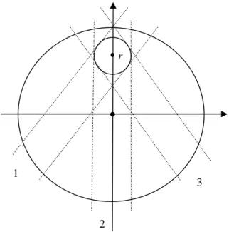
Figure 5 shows the section of a uniform charged ball with a radius a , inside which there is a small test body in form of a ball with a radius b.
Fig.5. The small ball is at a distance r from the center of the large ball.
The fluxes of charged particles of the vacuum field move along the paths 1, 2, 3, as well as other paths, passing the section of the small ball, which is at a distance r from the center of the large ball. If we replace the small ball with the cube of the same size, then in case of idealized cubic distribution it is enough to consider the vertical fluxes along the path 2. The fluxes of charged particles passing through the other faces of the small cube will be
2 1
3
symmetrical and will not influence the electric force. This means that with this approach we will take into account the fluxes along inclined paths 1 and 3 not directly, but indirectly. All these fluxes in case of vector summation will give the force, acting on the small ball and should be added to the force, calculated for path 2.
Let the volume of the small ball be equal to the volume of some cube. Then for the volume of
a cube with an edge s and for the absolute value of charge q of this cube we obtain the
relations: 3 3 4 3 b s , 3 b q e s , (10)
where is the concentration of charge in the small ball.b
Distribution (9) replaces the actual distribution of the charged particles of the vacuum field in space with the idealized cubic distribution, when only six fluxes of charged particles fall on the given cubic volume perpendicularly to the faces of the cube.
By analogy with (2) we can write the dependence of the fluence rate of the charged particles of the vacuum field on the distance traveled in the matter:
dD Ddx, DD0qexp (x). (11)
Let us first assume the charge q of the small ball in Figure 5 as negative and the charge of the large ball as positive.
The flux of charged particles falling from above travels the path
2 s
a r in the large ball with the concentration of charge in its matter, and reaches the small cube, with which wea replaced the small ball. According to (11) at this point the fluence rate decreases to the value:
1 0 exp 2 q a s D D a r .
Then the flux passes through the small cube with concentration of charge and decreasesb
again:
2 1exp ( b )
D D s .
The force from this flux of charged particles is proportional to the square of the face of the small cube and to the number of charged particles, which transferred their momentum per time unit to the cube matter:
2 2 1 ( 1 2) 1 exp ( ) 0 exp 2 q q b q a s F p s D D p s s D a r . (12)On the lower side of the large ball the flux of charged particles first passes the path
2 s a r to a small cube and then passes through the cube:
3 0 exp 2 q a s D D a r , D4 D3exp (bs).
The force acting on the small cube from this side equals:
2 2 2 ( 3 4) 1 exp ( ) 0 exp 2 q q b q a s F p s D D p s s D a r . (13)
2
1 2 1 exp ( ) 0 exp exp .
2 2 q q b q a a s s F F F p s s D a r a r
Since exponents in this expression are small enough, the exponents can be expanded in the small parameter by the rule: exp () 1 . With this in mind, we obtain:
2 3 0
2
q q q b a
F p D s r.
In this expression, we will take into account that the charge density of the large ball is given by the formula: q ea, and will use (10):
2 0 2 2 q q q q q p D r F e , 2 0 2 2 q q q q q p D e r F .
The force Fq acts on the small ball with the negative charge q in Figure 5 so that the force is directed toward the center of the large ball and oppositely to the radius vector r from the
center of the large ball to the small ball. By definition, the electric field strength is the ratio of the force, acting on the test body, to the charge of the test body. Then the vector of the electric field strength inside the large ball will be:
2 0 2 2 q p Dq q q q e F r E . (14)
In electrostatics, the vector of the electric field strength inside a uniform charged ball is determined by the formula:
0 3 q r E . (15)
From comparison of (14) and (15) we find the expression of the vacuum permittivity in terms of the parameters of charged particles fluxes in the cubic distribution approximation:
2 0 2 0 6 q q e p D . (16)
The difference between the used cubic (9) and spherical (1) distributions leads to the fact that the formulas for vacuum permittivity (16) and (6) differ by a numerical factor.
If the small ball in Figure 5 has not a negative charge but a positive charge q, then its interaction with the charge of the large ball should be considered in view of Figure 3 for the interaction of two positive charges. It means that it is necessary to introduce an additional coefficient in order to take into account the effect of increasing of the flux of charged particles.
As a result, the fluence rates D and1 D2 and the force (12) from the flux of charged particles falling from above on the small cube, by which we replaced the small ball, will change and be equal to:
1 0 exp ( ) 2 q a s D D a r , D2 D1exp (bs),
2 2 1 ( 1 2) 1 exp ( ) 0 exp ( ) 2 q q b q a s F p s D D p s s D a r . (17)Similarly, at the lower side of the large ball for the fluence rate and the force, instead of (13), we have:
3 0 exp ( ) 2 q a s D D a r , D4 D3exp (bs),
2 2 2 ( 3 4) 1 exp ( ) 0 exp ( ) 2 q q b q a s F p s D D p s s D a r . (18)The total force equals the difference between the forces (18) and (17):
2 1 2
0
1 exp ( ) exp ( ) exp ( ) .
2 2 q q b q a a F F F s s p s s D a r a r
Expanding the exponents by the rule: exp ( ) 1 , we find:
3 0
2 ( )
q q q b a
F p D s r.
Let us assume that the charge density of the large ball is given by the formula: q ea, and for the coefficient the relation holds: 2, which was found in the previous section. Then, with regard to (10), we obtain:
2 0 2 3 0 2 2 2 q q q q q q b a p D q r F p D s r e .
The force Fq is directed radially from the center of the large ball, and the expression for this force after dividing by the charge q leads to the electric field strength (14).
5. THE PARAMETERS OF THE FLUXES OF CHARGED PARTICLES OF THE VACUUM FIELD
We will estimate the energy density for cubic distribution of charged particles fluxes of vacuum field in space. Suppose there is a cube with an edge s , into which charged particles fly from six sides perpendicularly to the faces of the cube. The speed of charged particles is assumed to be equal to the speed of light, so that in the time s
c the cube will be completely
filled. In view of distribution (9) the number of charged particles in the cube will be:
3 0 6 c s D N c
. If the energy of one charged particle is Eq p cq , then with the help of (16) for the energy density of charged particles of vacuum field we find:
2 0 3 2 0 6 q c cq q q E N e p D s . (19)
Now we will use the spherical distribution (1) to estimate the energy density of charged particles of vacuum field. An empty sphere with radius R can be filled with charged particles in the time 2R
c , if the graviton fluxes are directed radially and correspond to the full
solid angle 4 . The number of charged particles inside the sphere will equal
0 8 q s ARB N c
. Multiplying this number by the energy of one charged particle and dividing
by the sphere’s volume we can find the energy density. In view of (6) and the condition 2 4 A R , we obtain: 2 0 3 2 0 3 3 24 4 2 q s sq q q E N e p B R . (20)
distribution (19), which emphasizes that our estimates are approximate due to the use of two idealized distributions.
Earlier in [5] we have applied the concept of the graviton field to calculate the Newton’s gravitational force between two bodies and the gravitational constant. This allowed us to estimate the energy density of the graviton field for cubic distribution and the rate of the energy flux of the graviton field in one direction:
2 35 0 3 2 4 6 7.4 10 g c n c g E N GM p D s J/m3, (21) 2 43 0 2 2 3.7 10 3 6 n c f g cGM c P E D W/m2,
here Eg p cg is the average energy of one graviton, pgis the average momentum of one graviton, D0 is the number of gravitons falling per unit time on unit area from one of the six
spatial directions in cubic distribution,
3 0 6 c s D N c
, G is the gravitational constant, Mn is
the mass of one nucleon of the matter, 5.6 10 50m2 is the cross section of interaction of gravitons and the matter.
The energy density in (21) is associated with the gravitational constant G and withc gravitation at the level of nucleons. Similarly, the energy density of the charged particles of the vacuum field cq in (19) is associated with the electromagnetic action of the field on each elementary charge eof the matter.
Further we will need the similarity coefficients, with the help of which in the theory of infinite nesting of matter [2], [6] we will calculate the physical quantities inherent in each particular level of matter. As the typical parameters of a neutron star we will take the mass equal to 1.35
Solar mass or 30
2.7 10
s
M kg and the stellar radius equal to Rs 12 km.
Dividing the mass of the neutron star by the proton mass Mp, we find the coefficient of
similarity in mass: s 1.62 1057
p M M
. Similarly, we calculate the coefficient of similarity
in size as the ratio of the stellar radius to the proton radius: s 1.4 1019
p R P R , here the quantity 16 8.73 10 p
R m in the self-consistent model of the proton [7] was used. We can estimate the minimum possible radius of the neutron star based on the ratio of the star volume
to the total volume of all the nucleons in the stars:
3 3 4 4 3 3 p s R R , 13 10.25 s p R R
km. A star with the radius of 12 km exceeds this limit, there are some gaps between the nucleons and the nucleons remain to be independent particles.
The coefficient of similarity in speed equals the ratio of the characteristic speeds of the matter inside the star and the proton, respectively. For the star the characteristic speed Cs is calculated from the energy equality from the standpoint of the general principle of equivalence of mass and energy, generalized with respect to the absolute value of the total energy to any space objects:
2 2 2 s s s s kGM M C R , 6.8 107 2 s s s kGM C R m/s.
Similarly, we find for the proton the equality of the characteristic speed of its matter and the speed of light: 8 2.99 10 2 p p p k Γ M C c R m/s,
while 2 29 0 1.514 10 4 p e e Γ = M M m 3
·kg-1·s-2 is the strong gravitational constant,
calculated from the equality of electric and gravitational forces in the hydrogen atom, is0 the vacuum permittivity, Me is the electron mass and according to [7] for the proton
0.62
k . Hence, the coefficient of similarity in speed is equal to: s 0.23
p C S
C
.
As it was shown in [2], the ratio of the absolute value of strong gravitation energy density to the electromagnetic energy density of the proton is equal to the ratio of the proton mass to the
electron mass p
e M
M . Indeed, for the energy of the fields and their ratios, in view of the
definition of the strong gravitational constant Γ , we have:
2 p g k Γ M E R , 2 0 4 e k e E R , 2 0 2 4 g p p e e E Γ M M E e M
. We believe that the same ratio exists for the energy densities of
graviton field and charged particles of the vacuum field, which allows us to estimate the energy density of charged particles of the vacuum field:
32 4 10 e cq c p M M J/m3. (22)
Let us substitute (22) into (19), using the value of from (21), and take into account thec proximity of the proton mass and the average mass of a nucleon Mp Mn, as well as the definition of the strong gravitational constant in the form
2 0 4 p e e Γ = M M . This gives an
estimate of the cross section of interaction of the charged particles of the vacuum field with the charged matter:
30 0 0 0 1 2.67 10 4 p c e p e cq M e Γ e e M M M G G m2. (23)
This cross section has a value that almost exactly coincides with the geometrical cross section of a nucleon and significantly exceeds the cross section 5.6 10 50m2 of interaction of gravitons with the matter. In order to find the significant difference between and , we will express from (22), usec cq from (19) and take into account the definition of Γ:
2 2 2 2 0 4 p p p c cq e e M e M Γ M M M . (24)
From comparison of (24) and (21), provided that Mp Mn, it follows that if in (21) we pass from the cross section to the cross section , then at the same time it is necessary to substitute the gravitational constant G with the strong gravitational constant Γ . In (24) the energy density of the graviton field at the level of nucleons is fully expressed in terms ofc the parameters of the nucleon level of matter. Similarly, in (19) the energy density cq of the charged particles of the vacuum field is expressed in terms of the parameters of the nucleon level of matter. In this case, both in (19) and (24) the same cross section of interaction of the vacuum field particles with the matter consisting of nucleons is used. Note that in [4] it was found that the cross-section of the interaction between the gravitons and the matter of nucleons must be equal by the order of magnitude to the cross-section of the proton.
By analogy with (24) for the graviton field at the stellar level we can write:
2 2 4 s s s GM .
If in this expression we shall consider the following relations in accordance with the dimensional analysis, coefficients of similarity and (24):
2 PS G = Γ , Ms Mp, 2 s P ,
then we obtain the relation
2 34 3 2.3 10 s c S P
J/m3, in which the energy density of
graviton field at the stellar level , needed to keep the matter in neutron stars, linked to thes energy density . Since the energy densityc is required for the integrity of the nucleonsc in the field of strong gravitation, then c s.
In view of (16), (19), (22) and the relation Eq p cq , for the rate of the energy flux of charged particles of the vacuum field in one direction we find:
2 40 0 2 0 2 10 6 6 cq fq q q c c e P E D W/m2. (25)
Due to the fact that the above-mentioned energy density cq of charged particles of the vacuum field is less than the energy density of graviton field in (21), the rate of thec energy flux of charged particles of the vacuum field Pfq is less than the rate the energy flux of the graviton field Pf .
6. THE ESTIMATES OF FORCES AND ENERGIES
In [2] and [6] the assumption is made that some neutron stars – magnetars can have a positive electric charge of up to Qs eS P 5.5 10 18 C, where e is the elementary electric charge and the similarity coefficients are used in accordance with the dimensional analysis.
5 0 6.6 10 4 s p e s eQ E R
J or 4 10 24eV. The corresponding electric force will be equal to
2 0 55 4 s p e s eQ F R
N. It is assumed that it is precisely the electrical energy in the magnetar
field that is the energy source of high energy cosmic rays.
For the absolute value of the gravitational energy of the proton on the surface of the magnetar
similarly we have: p g p s 2.5 10 11 s GM M E R
J. This energy and the gravitational force,
associated with it, are clearly not enough to keep the proton, on which the repulsive force is acting from the entire charge of the magnetar. However the magnetar looks like a huge atomic nucleus consisting of a number of closely-spaced nucleons. Between nucleons there is strong interaction, which holds them together. In the gravitational model of strong interaction [6] the idea of strong gravitation is used to describe the strong interaction. The nucleons in the atomic nuclei are attracted to each other by strong gravitation and repel from each other by means of the torsion field, which arises from the rapid rotation of the nucleons. According to the Lorentz-invariant theory of gravitation [1-2], the torsion field arises similarly to the magnetic field in electromagnetism, and in the general theory of relativity it corresponds to the gravitomagnetic field. The balance of attractive and repulsive forces, arising from strong gravitation, can be responsible for the integrity of the atomic nuclei, as well as for the integrity of the charged neutron star.
We did the estimates of forces and energies in the atomic nuclei in [6]. For example, the nickel nucleus 62
28Ni consists of A62 nucleons, among which there are 28 protons and 34
neutrons. The mass of this nucleus is MN 1.028 10 25kg, and the radius is obtained from experiments on the scattering of electrons by the formula: RN R A0 1 34.9 10 15m, where
15
0 1.23 10
R m. Based on these data we will estimate the force, acting from the nucleus on
the proton located on the nucleus surface, with the help of strong gravitation:
6 2 1 10 p N p N N Γ M M F R N.
The surface of the magnetar as a neutron star apparently consists of the nuclei of such elements as iron, nickel and heavier nuclei, since their binding energy per nucleon is maximum. If the proton was near one of these nuclei on the magnetar surface, the force Fp N would keep the proton, acting against the force of electrical repulsion Fp e 55N from the magnetar charge. But the concentration of nuclei on the stellar surface is such that the proton
on the average will be located somewhere between the nuclei at a distance r from them.
To keep the proton the condition p p2 N p e
Γ M M
F F
r
must hold, which implies that
13
7 10
r m. For a cube with the edge 2r , at the corners of which there are 8 nuclei 6228Ni, and the proton is in the center of the cube, the matter density is equal to
11 3 3 10
N M
r
kg/m3. The matter density on the magnetar surface must exceed this value,
so that the condition of stability with respect to electric forces is satisfied. On the other hand, the estimates in [8] of the matter density in the crust of the neutron star imply that at a density of 2.7 10 11 kg/m3 and more the nuclei 6228Ni begin to decay. Consequently, heavier nuclei must prevail in the magnetar crust, in particular, a typical nucleus according to [8] is 10535Br. From these calculations it follows that the magnetar charge is almost the maximum charge that the star can have without loss of its integrity. And the main contribution into the stability of a star is made by not ordinary but strong gravitation, acting at the level of atomic nuclei. With the help of the similarity coefficients we can calculate the mass, radius and charge of the praon – the particle, which relates to the proton, as the proton relates to the magnetar:
84 1 10 p pr M m kg, rpr Rp 6.2 10 35 P m, 57 4.6 10 pr e q S P C. If the praon is
located at the surface of the proton, its electrical energy and gravitational energy in the strong
gravitational field will be equal: 51
0 7.6 10 4 pr pr e p q e E R J, 67 2.9 10 pr p p g p Γ m M E R J.
The ratio of these energies is the same as the ratio of the electric energy of the proton at the surface of the magnetar to the gravitational energy of this proton in the gravitational field of
the magnetar. In the substantial model of the proton and neutron, presented in [6], it is assumed that the nucleons consist of neutral and charged praons, just as neutron stars consist of nucleons. In addition, by analogy with the composition of cosmic rays, consisting mainly of relativistic protons, we can assume that the charged component of the vacuum field can consist of praons accelerated by positively charged atomic nuclei up to high energies.
At the present time cosmic rays are registered with energies up to Er 6 1019eV or 9.6 J per nucleon [9]. Assuming that this is the energy of the accelerated proton, we will divide it by the coefficient of similarity in energy and will find the corresponding energy of the praon:
55 2 1 10 r pr E E S
J. Equating this energy to the energy Eq of a charged particle of the vacuum field, we can estimate the concentration of these charged particles as the concentration of relativistically moving praons. In view of (19) and (22) we obtain:
87 3 4 10 cq cq c pr q pr N n s E E m-3.
Multiplying this concentration of charged particles by the charge of one praon qpr and the speed of light, we can estimate the density of the current in the vacuum in one direction, which arises from the flux of positively charged praons in one direction at cubic distribution:
39
5.5 10
pr pr
j n q c A/m2.
Beside the current density j, we should expect another similar current density j in the same direction, which arises from the flux of negatively charged praons. This should ensure a certain degree of vacuum electroneutrality and existence of electrical forces of repulsion and attraction.
Now we will consider the question of neutron star’s matter permeability for gravitons and
similarly to (2) have the form:
0exp ( )
BB n x , Bq B0qexp(x).
If the neutron star has a radius of 12 km and a mass of 1.35 solar masses, then the average
concentration of nucleons will equal 3 3 2.2 1044
4 s n s M n M R
m-3. The average concentration
of the positive charge in the magnetar is 3 3 4.7 1024
4 s s Q eR m-3. Assuming that 2 s 24
x R km, for the exponents in view of (21) and (23) we find: n x0.3,
0.007
x
. It follows that if we put three neutron stars in the way of the flux of gravitons,
the flux will reduce approximately by a factor of e , wheren en 2.71828...is the base of the natural logarithm. But for the flux of charged particles of the vacuum field in order to reduce it noticeably we need to put in a line about 140 magnetars.
This difference in fluxes allows us to explain the saturation effect of the specific binding energy, when the nuclear binding energy per nucleon, depending on the number of nucleons in nuclei, first increases, reaching a maximum of 8.79 MeV per nucleon for the nucleus 6228Ni, and then begins to decrease. For light nuclei the increase in the specific energy agrees well with the increase of the specific gravitational energy of the nucleus in the strong gravitational field, when the energy increases in direct proportion to the square of mass and in inverse proportion to the radius of the nucleus. The saturation effect comes into play in the range of 17 to 23 nucleons, forming the nucleus. Besides, adding a new nucleon to the nucleus increases the energy not proportionally to the square of mass, but to a lesser extent. This is due to the fact that gravitons of strong gravitation cannot permeate the nucleus with a lot of nucleons, as is evident from the exponent. Each new nucleon is simply pressed to the nucleus from the outside by the strong gravitation, until for the large nuclei this force reaches the maximum, conditioned by the pressure of the graviton flux. However, the charged particles of the vacuum field in these conditions have almost 50 times larger path length, and therefore the
positive electrical energy of the nucleus’ protons further decreases the negative gravitational
energy of the nucleus, making the main contribution into the observed decrease in the specific binding energy of massive nuclei.
Earlier in [4] we estimated the maximum force between two stellar objects:
4 43 m 2 2 10 16 c F k G N,
where k 0.6 for the case of uniform density of each object, and it is assumed that the graviton fluxes are fully retained by these objects, which are located close to each other.
A similar expression for the maximum force at the nucleon level of matter, after replacing the gravitational constant by the strong gravitational constant, in view of the coefficient of similarity in speed S 0.23 has the form:
4 6 m 2 4 5 10 16 c f k S Γ N.
We should note that the corresponding ratio of the gravitational energy and the force between two protons to their electrostatic energy and force is equal to the ratio of the proton mass to the electron mass. Indeed, for the forces and their ratios in view of the definition of the strong gravitational constant 2 0 4 p e e Γ = M M , we have: 2 2 p g Γ M F R , 2 2 0 4 e e F R , 2 0 2 4 g p p e e F Γ M M F e M
. We can explain this by the fact that in the expression for Bq the
exponent for the flux of charged particles of the vacuum field in the magnetar and hence in the proton is less than the corresponding exponent for the flux of gravitons in the expression for B. The gravitons are retained in the proton matter more than the charged particles of the vacuum field, and therefore the gravitational force is greater than the electric force.
After passing from dense and charged objects such as magnetars and protons to the bodies surrounding us the situation with the ratio of forces is changing. The gravitational force decreases rapidly with decreasing of the mass of bodies, and we can hardly influence it. However, by changing the charges of bodies we can change their electrical interaction, so that the electric force can be many times greater than the gravitational force between these bodies. This can be seen from the ratio of the electric and gravitational forces for two identical bodies
with the mass m and charge q , which is proportional to the squared charge:
2 2 0 4 e g F q F Gm .
Let us take for example two iron balls with the radius r5cm each. With the density of iron 7874 kg/m3 it gives the mass of each ball of approximately 4.1 kg. For the equality of the gravitational and electrical forces it is enough to charge the balls up to
10 0
4 3.5 10
qm G C, so that the potential of each ball reaches the value
0 63 4 q r
V. Let us estimate the electrical energy of the praon, flying near the ball, taking into account that above we estimated the charge of the praon with the value
57 4.6 10 pr e q S P
C: Epre qpr 3 1055J. On the other hand, the energy of a praon,
regarded as a relativistic particle similar by its properties to cosmic rays, has been found
above in the form: r2 1 10 55
pr E E S
J. Comparison of these two energies allows us to
make the following conclusions. Firstly, even weakly charged bodies, which interact at the level of low gravitational force, can influence the motion of praons near them and deflect them aside. This substantiates the pattern of motion of the charged particles of the vacuum field near the charged bodies in Figures 1-3 and our calculations of the electric force. Secondly, if we decrease the charges and increase the sizes of bodies, there can be deviations from the Coulomb law. However, these deviations should be distinguished from the gravitational force, which in this case becomes greater than the electric force.
Coulomb law, it is desirable that the condition of small potentials is satisfied 0 22 4 pr pr E q r q
V. To reduce the dependence on the gravitational force, there are the
following conditions FeFg or qm 40G . Hence for the corresponding electrical
potential of one ball, we have:
0 22 4 m G r V or 28.4 m
r kg/m. For the iron balls it
gives r2.9 cm, m0.8 kg. Another complication in the experiments for finding
deviations from the Coulomb law occurs due to the fact that in conductive bodies the
uncompensated charges are located in the thin layer on the bodies’ surface, with a thickness of
the order of 1 or 2 atomic layers. Free electrons easily go out of the equilibrium position in the external electric field, either repelling or being attracted to the source of the external field, thereby changing their concentration on the body. Due to this, in two interacting charged metal balls additional electrical forces appear, which are usually calculated by the method of images.
7. INTERACTION OF THE BODY’S CHARGE WITH THE VACUUM FIELD
The Coulomb law, due to the presence of charged particles in the vacuum field, can be
explained with the help of Le Sage’s model. However, not only the fluxes of charged particles
influence the interaction of charged bodies, but the charges of bodies themselves influence the fluxes of charged particles around the bodies. One example of this influence is deflection of the charged particles from their trajectories, as it was described in the previous section. In addition, each charged body achieves a certain balance of energy and momentum during interaction with the vacuum field.
Let us consider the energy density of the charged particles of the vacuum field inside the charged body and near it. Suppose there is a body in the form of a cube with an edge s . The number of charged particles D per unit time through a unit area during particles’ motion in
the matter decreases according to formula (11). During time s
c six fluxes of charged
change up to the value: 1 0qexp( ) D D s , 3 0 6 exp ( ) q s D N s c ,
where N is the number of charged particles that passed through the cube.
If charged particles flew through the same empty volume, the number of charged particles
coming out would be
3 0 0 6s Dq N c
. Consequently, the number of charged particles, which
interacted with the matter of charged body during time s
c, equals:
3 4 0 0 0 6 6 1 exp ( ) q q s D s D N N N s c c .As it was shown in [5], almost all the energy of the graviton field, which interacts with the matter, is re-emitted back to the graviton field, without heating the bodies significantly. This also applies to the fluxes of charged particles the vacuum field, that transfer their momentum to the matter with return of the energy back to the vacuum field.
Let us estimate in view of (19) the energy density of those charged particles that interact with
the bodies’ matter:
3 q m cq N E s s . (26)
From (26) we will calculate the luminosity of charged particles of a body in the form of a
cube, multiplying by the volumem s3 and dividing by the time s
concentration in terms of the charge, in view of (19) we have: 3 Q es , 2 3 0 q m cq cq Q ceQ P s c s c c e . (27)
From (27) it follows that the luminosity Pq of the charged particles, understood as the luminosity of those charged particles fluxes that interacted with the charged matter of body
and gave their momentum to it, is proportional to body charge Q. This means that the body
charge can be expressed in terms of the parameters of the charged particles fluxes interacting with the body.
In (27) there is a product n s3 equal to the number of uncompensated elementary charges in the body under consideration. Then the charged particles luminosity per one elementary charge, in view of (19), (22-23) will equal:
11 1 3 6 0 6 0 3.2 10 q cq q q q q P P c p D c E D s W. (28)
The ratio of the luminosity P to the average energy of a charged particle1 Eq p cq gives the number of charged particles that interact with one uncompensated elementary charge of matter per unit time and gave their momentum to it. According to (28), this number of charged particles is equal to the product 6D0q , while the cross section characterizes the
effective area of elementary charge’s interaction with charged particles, and the coefficient 6
is associated with the six sides of cubic distribution of charged particles fluxes D0q in (11). Expression (27) can be given a different meaning, if we assume that the area of the cube face is connected with the cross section by the following relation: s2 k N1 , where k is1
some numerical coefficient, N is the number of uncompensated elementary charges in the
2 1 2 0 q ck Q P s .
This relation shows that the emission rate is proportional with accuracy to a coefficient k to1
the electric energy of the charged body, derived from the body in the time s
c of passing the
body characteristic size by the charged particles.
We note one more aspect concerning the interaction between the electromagnetic and gravitational fields. The concept of the general field [10] shows that the vector fields, including the electromagnetic and gravitational fields, are the components of one general field. And in case if the theorem of equipartition of the energy is satisfied, the equations of particular fields no longer depend on each other and are similar in form to the Maxwell equations. If the fields interact with each other, then in the Hamiltonian it is manifested in the terms with the field energy, where the cross-terms with the products of different field strengths appear. This is possible, for example, in non-stationary processes in the systems that have not reached equilibrium. From the viewpoint of the vacuum field, it means that in stationary conditions the gravitons and charged particles of the vacuum field interact with the matter relatively independently, creating gravitational and electromagnetic forces. If there is no equilibrium in the system, then the kinetic energy of matter and the energies of some fields are transformed into the energy of other fields, and the exchange of energies between gravitons and charged particles in the vacuum field is possible as well. This leads to the cross-terms in the system’s energy.
8. PHOTONS AND PRAONS
In this section we will try to specify which particles can be responsible for electromagnetic phenomena. The charged particles of the vacuum field not only lead to the electric forces in the Coulomb law, but should be part of the photons, i.e. the electromagnetic quanta emitted by atoms. Let us consider, for example, a photon with the wavelength 1.21567 10 7m and
the angular frequency 2c 1.54946 1016
s-1, arising in the hydrogen atom in the
transition of an electron from the second to the first level in the Lyman series. The probability of this transition equals A2 4.699 10 8 s-1 [11], which gives the average lifetime of an
electron at the second level 2 9
2
1
2.1 10
A
s, as a measure of duration of photon emission
during the transition. In quantum mechanics [12] there is a formula for the oscillator’s oscillations decay time in en times, where en 2.71828... is the base of the natural logarithm, with the help of which we obtain the following estimate:
9 2 2 0 12 1.3 10 e o cM e s.
where is the vacuum permeability.0
The duration of photon emission can be calculated directly within the Bohr model of a hydrogen atom. In this model, the electric force between a proton and an electron acts as a centripetal force in the electron’s rotation around the nucleus in the form of a proton. In this rotation, the electron must emit an electromagnetic wave, since it is constantly accelerated towards the nucleus. The formula for the charge emission rate during its rotation is well known, which allows us to relate the electron velocity and the effective force acting on the electron from emission. Moment of this force decreases the angular momentum of the electron, leading to a decrease in the radius of rotation. Hence we can derive the dependence of the radius on the time [6]. From this dependence we find the duration of photon emission as the time of transition of an electron from the second to the first level of energy. Given that the average radius of the electron rotation on the second level equals r2 4aB, and the average radius of the electron rotation on the first level is the Bohr radius r1aB, we have the following:
2 2 3 2 3 3 10 0 2 1 4 4 9.8 10 e c M r r e s. (29)For the instantaneous power of electromagnetic emission we obtain the formula:
6 3 3 3 2 4 0 96 r e e e P c M r .
This implies a strong dependence of the emission rate on the current radius r of the electrone
rotation, which is inversely proportional to the fourth power of this radius. It turns out that the main photon energy is emitted when the electron approaches the lower energy level.
Knowing the emission duration we can find the length of the photon c. To calculate the volume of the photon we also need its midsection. In the first approximation, we assume that the mean radius of the photon equals r4aB, which is equal to r . We note that in the2
substantial model of electron [6], it is considered as a thin disk that has on the main energy level the inner radius 0.5aB and the outer edge 1.5a , and the Bohr radiusB r1 aB is obtained as a certain characteristic radius of the disk and the average radius of the electron rotation. On the second level, the outer edge of the electron disk is greater than the average radius of the electron rotation r2 4aB on this level. With this in mind, the volume of the photon will equal: V r216a cB2 .
Further on we will use a simplified model of photon from [2], [13], according to which the
photon consists of charged particles, the rotation of which around the photon’s axis creates the
angular momentum of the photon. In addition, inside the photon as well as in the electromagnetic wave there must be mutually-perpendicular periodically varying electric and magnetic fields. Electromagnetic energy of the photon consists of the equal electric and
2 2 2 2 2 2 0 0 0 0 1 2 2 2 e m E B E c B E , since in the wave EcB. The electric
field strength E inside the photon will be characterized by the amplitude E . The field0
inside the photon oscillates, varying from zero to the peak value, so for the average density of
the electromagnetic energy of the photon, we assume that 0 2
0
2
em E
. We also assume that
the photon energy is equally divided between the mechanical energy of the charged particles and the electromagnetic energy. The photon energy W is proportional to the Dirac
constant and the angular frequency . Dividing the photon energy by the photon volume,
we obtain the energy density, which can be equated to the doubled density of electromagnetic energy inside the photon:
2 em W V , 2 0 0 2 E r c . (30)
Substituting in (30) the photon angular frequency 1.54946 10 16s-1, the duration of the
photon emission from (29) and the photon radius r4aB, we estimate the amplitude of
the electric field strength inside the photon: E0 2.1 10 6V/m. For comparison, the proton
creates at the Bohr radius the electric field strength 2 11
0 5.1 10 4 B B e E a V/m.
From the mechanical point of view we can consider in a simplified way the photon as a long thin cylinder, rotating with the angular frequency . If inside the cylinder there are N particles, each of which has a relativistic mass m, then in case of uniform distribution of
particles the angular momentum of the cylinder must be equal to the Dirac constant, as it is supposed for all photons:
2
1
2N mr
From (31) it follows that the mechanical energy of the particles’ rotation, calculated as half the product of the angular momentum and the angular velocity of rotation, is equal to the
half of the photon energy: 1 1
2 2
r
W W . The other half of the photon energy must be the
electromagnetic energy, which was taken into account in (30). Since the angular momentum of the electron in the atom is quantized and proportional to , from (31) it follows that the total relativistic mass N m of the charged particles rotating inside the photon must be of the order of the electron mass, in order to ensure the angular momentum of the photon. However, the mass N m is only a small part of the mass of the entire flux of charged particles of the vacuum field, that pass through the electron disk per time of the photon emission from (29). The total relativistic mass of particles of the entire flux per time is expressed by the product of the energy flux rate (25), the time and the area of the electron disk , and then dividing by the square of the speed of light in order to pass from ther2
energy to the mass:
2 5 2 3.1 10 fq r P c
kg, which is much greater than the electron mass.
Let us consider the motion of some charged particle inside the photon, located on the radius
r . This particle rotates at a certain velocity v around the axis of the photon, and besides it moves at the speed of light, as well as the photon, in the direction of its propagation. For the
particle’s period of rotation we can write:
2 2 r T v c , v r . (32)
In this model of a photon, there is a relationship between the centripetal force, required for the
particle’s rotation, and the electric force, exerted on the particle with the charge q and the