Calibration of Building Simulation Models: Assessment of Current
Acceptance Criteria
Roberto Ruiz, Vincent Lemort
University of Liège
Abstract
In this paper, the most used acceptance criteria in calibration of building simulation models are introduced and tried out by means of a practical exercise. In order to simplify the process of obtaining “simulated data” and to avoid carrying out a formal calibration procedure; two yearly testing profiles (hourly time scale) are created from real building electrical metered data (¼ hour profile). Both testing profiles represent two model responses that could possibly be obtained in a common calibration procedure.
The objective of this work is to test the capabilities of the method to determine (1) the model adequacy to represent an existing situation; (2) the reliability of the model when predicting a future or different scenario and also (3) the ability of the method to orient the practitioner to upgrade the model when it provides a non-satisfactory response.
To do this, the real accuracy of both testing profiles is verified by means of a complementary statistical bin analysis. This crosschecking analysis allows highlighting the strengths and weakness of the current criteria and determining whether they need to be revised, modified or complemented. At the end of the analysis, it is concluded that the capabilities of the current acceptance criteria are limited because don’t provide any satisfactory answer, indication or clue for none of the three points aforementioned and some other complementary tests (such as bin analysis) must be implemented and performed in order to properly declare a model as calibrated.
Introduction
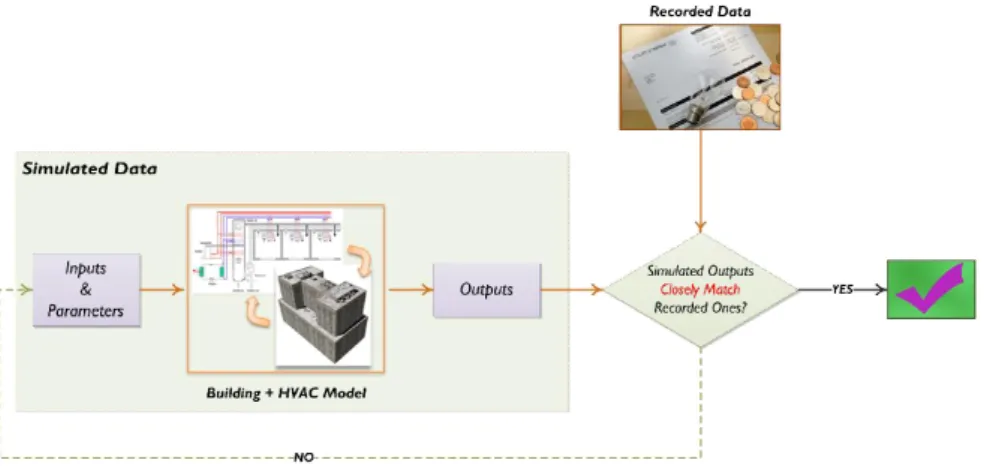
In building modeling and simulation, calibration consists in adjusting or “tuning” the parameters of an existing building model through several iterations until it agrees with recorded energy use and demand data within some predefined criteria (adapted from [1]). The process involves the use of a computer simulation tool to create a model of energy use and demand of the facility. This model is adjusted over a reference period, which is usually called “baseline period”. Figure 1 shows a generic scheme of the process.
Whole-building calibrated simulation is an approach proposed by the three major standards of energy performance measurement and verification for determining ECOs savings [2],[3],[4]. Its use is recommended when the energy impacts of ECOs are too complex or costly to evaluate by means of measurements. While this is the most common use, it can also be applied to performance analysis in other stages of the building life cycle such as: commissioning, continuous performance verification, fault detection, etc.
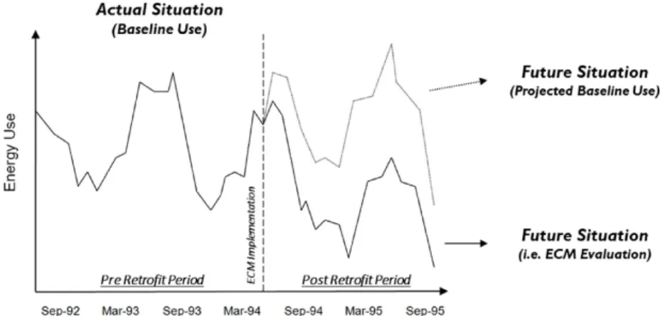
Regardless of the purpose for which it is required, the ultimate goal that must fulfill any calibrated simulation model is: to represent accurately the energy use and demand of an existing building within
a reference or baseline period so that it is able to predict accurately the energy use and demand for a future or post retrofit period under the same or different conditions (i.e. weather, control strategies,
HVAC equipment replacement, etc.). A representation of this issue is illustrated in Figure 2.
Figure 2
-
Determining savings (adapted from ASHRAE,2002)In the related literature, it can be found several approaches and methodologies applied to real case studies which show a good agreement in terms of accuracy when representing an existing situation; however, no study to date presents any evidence about the issue of whether this achieved accuracy can be transferred to predictions of a new scenario (i.e. projected baseline use and/or evaluation of intended ECM savings). Despite this issue is of great importance; some of the most important guidelines such as ASHRAE (2002) completely ignore this aspect [5].
In order to propose a solution to this issue, it is imperative to understand the overall process (Figure 1) and identify the main barriers that attempt against the successful completion of the calibration process (Figure 2). In practice, they can be summarized into two main constraints:
1. To common building energy data is a highly under-determined problem that would result in a non-unique solution [6].
2. The definition of accuracy criteria is a complex issue and, to date, it is impossible to determine how close a tolerance needs to be to fulfill the calibration objective [1].
The under determination is an inherent condition that is present in the whole calibration process and cannot be bypassed. In mathematics, a system of linear equations is considered underdetermined if there are more unknowns than equations. It means that an infinite combination of unknowns may satisfy a given set of equations.
So in building calibration, if the acceptance criteria are not able to identify the real correctness of a set of unknowns even if the they are providing a response within a desired tolerance range for an existing situation, then the predictions of the model for a future situation will not be reliable and therefore the calibration targets are not being achieved.
This paper covers and tries to give an answer to issue. It starts presenting the current and most used acceptance criteria. Then a complementary evaluation method is proposed, tested and the obtained results of this evaluation are confronted with some requirements that a model should fulfill. All this in
order to: determine the suitability of the acceptance criteria and establish how their results must be interpreted.
Current Acceptance Criteria
The most used acceptance criteria to determine whether a building simulation model may be considered calibrated or not, consist in calculating and comparing (with respect to a maximal tolerance) 2 statistical indexes: Normalized Mean bias error (N ) and Coefficient of Variation of the Root Mean Square Error ( ( )).
The first of the indexes, the Normalized Mean Bias Error (N ) is defined as the mean difference between the measured data values and model simulated values, normalized by the mean value of the measured data [7].
=
∑
−
M
(1)
Where: is the measured value during the period; is the simulated value during the period; is the measured average during the period and is the number of available data points (or periods)
measures how close the energy use or demand predicted by the simulation model corresponds to actual building data. The main drawback of this index is that it does not capture effects where positive and negative errors cancel each other out (offsetting errors).
Thus, an index that captures offsetting errors is necessary. This is the Coefficient of Variation of the Root Mean Square Error (CV(RMSE)) wich corresponds to a normalized measure that quantifies the degree of dispersion of a set of predicted values around the mean of the observed values. Notation is the same as shown above.
(
) =
∑
(
−
)
(2)
So, according to these criteria, the combination of and the ( ) can determine how well the model predicts whole-building energy use. The lower the and ( ), the better the calibration.
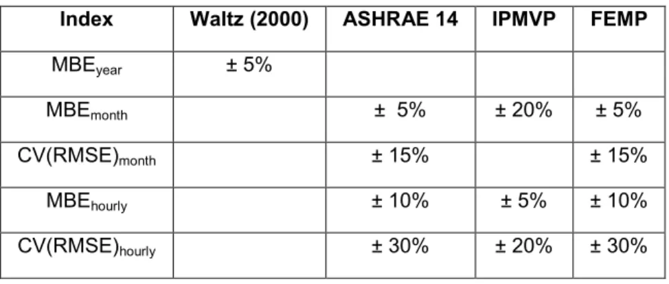
In practice, both indexes are evaluated for different end uses (usually electricity and fuel) and at different time scales (annual, monthly, hourly, etc.). Table 1 specifies the acceptable tolerances proposed by the three standards dealing with calibration [2],[3],[4].
Table 1 - Commonly used calibration tolerances
Index Waltz (2000) ASHRAE 14 IPMVP FEMP
MBEyear ± 5%
MBEmonth ± 5% ± 20% ± 5%
CV(RMSE)month ± 15% ± 15%
MBEhourly ± 10% ± 5% ± 10%
In addition to the calculation and comparison of these statistical indexes, some other complementary techniques have been proposed by different authors. For example, to enlarge the set of tolerances depending on the energy uses (lighting, cooling, heating, fans, etc.) and tuning periods (monthly, daily, hot period, cold period, etc.) [1].
US DOE (2008) [3] proposes the use of any or all of four graphical comparison techniques summarized in Bou-Saada and Haberl (1995) to compare a simulation's output with real data. These techniques are: hourly loads profiles, binned interquartile analysis using box-whisker-mean plots, weather day-type 24-hour profile plots and three-dimensional surface plots. Some of these techniques require significant post-processing of data and in this paper are not discussed.
Finally, according to the current acceptance criteria, if a model is able to provide results within the proposed tolerances for and ( ) for hourly, monthly and annual timescales, then might be declared as calibrated and its predictions may be considered as accurate and reliable. In the next sections this approach is tried out.
Material and Method
Proposed AnalysisThe proposed analysis considers the evaluation of both statistical indexes ( and ( )) at different time scales (annual, monthly and hourly) in order to determine the adequacy level of a “hypothetical model response” with respect to real metered data. For this purpose, two electrical ¼ hour profiles (corresponding to reference building) have been taken, handled and used as model response (simulated data) and metered data.
The term “model response” makes reference to a whole-building electrical hourly profile which can be considered as a candidate solution obtained during a calibration procedure and for which, is required to determine its actual accuracy and reliability. The reason why this approach was chosen is certainly to avoid performing a calibration procedure (a matter of time) but also because, the quality of the candidate model response is previously known and the way how this aspect is shown by the acceptance criteria indexes is required. In this analysis two “model responses” are tested. Details about how they were obtained are given below.
Reference Building
The reference building (commonly known as DM28) corresponds to a tertiary building located in the city center of Brussels, Belgium. It accommodates the European commission for energy and transport.
The building comprises 10 stores above ground (9 corresponding to offices and 1 to technical rooms) and 3 underground parking. Its fully enclosed area is about 18700 m2.
According to building services and operating schedules, the building can be divided in 3 zones: The first one corresponds to the entrance hall of ground level (about 150 m2), the second one to office’s floors +1 to +8 and the remaining ground level (about 10200 m2) and the third one to the 3 underground parking (about 7600 m2). Building services and main electrical consumers comprise: artificial lighting, office’s appliances and HVAC systems. Table 2 shows the operating schedule per service and zone.
Table 2 - DM28 operating schedules
Service Entrance Hall Offices Parking Day Type
Lighting and appliances 06:00 – 22:00 06:00 – 22:00 (*) 06:00 – 22:00 Weekdays 10:00 – 19:00 10:00 – 19:00 (*) – Weekends and Holidays HVAC system 06:00 – 22:45 08:00 – 20:00 08:00 – 20:00 Weekdays 10:00 – 19:00 – – Weekends and Holidays
(*) In this zone, lighting is manually controlled by occupants but out of this period BEMS shuts it off automatically.
Artificial lighting is present in the whole-building being the “entrance hall” negligible to the total consumption due to the small surface it serves. Appliances are only present in “office’s zone”. HVAC system serves almost all the building excepting technical rooms. It comprises: Hot water production (3 gas boilers and auxiliaries), cold water production (2 water cooled chillers and their respective cooling towers and auxiliaries), mechanical ventilation (5 AHUs and 4 extraction fans), terminal units (4 pipes FCUs and hot water convectors) located at “office zone” and 2 air heaters located in parking spaces. In order to complement the schedules shown in Table 2 and to understand better the HVAC operation and its impact on the electric usage, it must be indicated:
The heating plant is stopped when outdoor temperature goes over 16°C (summer limit temperature). The three boilers and all the circulators and pumps are started (24/7) when outdoor temperature goes below 3°C to avoid freezing. The cooling plant is automatically switched off as soon as the outdoor temperature is below 14°C.
Figure 4 shows electrical power demand profile recorded for year 2009. It has been obtained from a ¼ hour profile belonging to reference building.
Figure 4 - Whole-Building Electrical power demand – Surface plot arranged by weeks
0 20 40 60 80 100 120 140 160 180 0 20 40 60 0 200 400 600 Wee k of Y ear
Whole Building Electrical Power Demand (Hourly Profile) Hour of Week W B EP D [ kW h /h]
Weekly profile plotted in Figure 4 shows a clear impact of BEMS in the repeatability of 5 weekdays and 2 weekend daily profiles, the characteristic shape and order of magnitude of each one; and also a seasonal effect can be perceived when going to through the calendar year (week of year axis). This fact verifies the information of operating schedules provided in Table 2.
Characterizing Daily Load Profile
Daily load profile experiences a very clear behavior for both types of days. Even if weekdays seem to be very influenced by occupants’ actions (because of the load shape) is also true that several periods during the day can be recognized where some consumptions must surely be allowed or not in function of occupants’ presence.
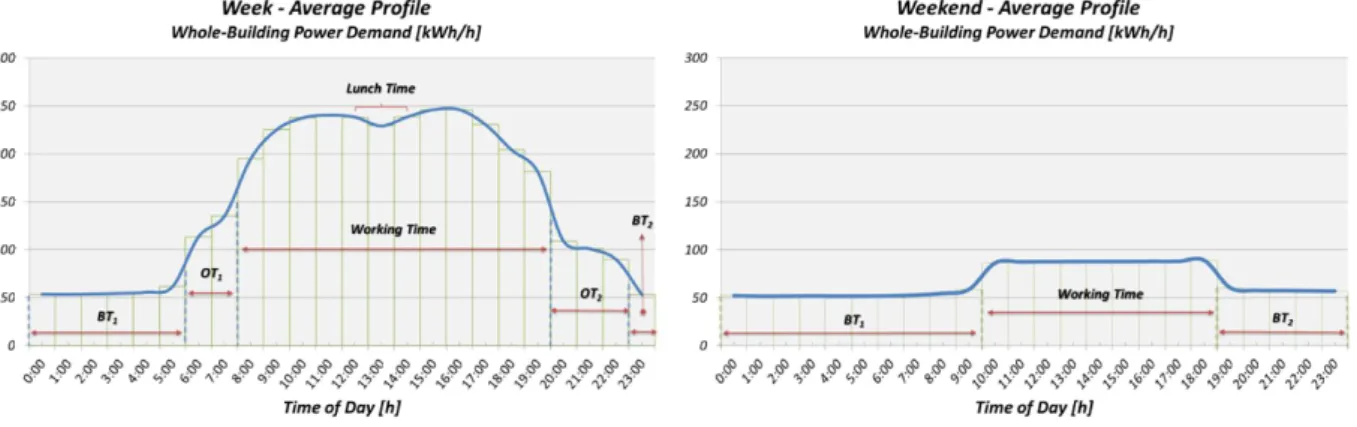
Figure 5 shows two average profiles (week and weekend) containing some recognized daily periods.
Figure 5: Electrical daily load profile for week and weekend days respectively.
According to profiles seen in Figure 5, some different periods can be easily recognizable during a working day. They are:
1.
Working time (WT): period corresponding to the biggest part of the day that also comprises an “intermediate” break time period (coffee, lunch, etc.). It is normally defined by the company and corresponds to the “nominal” hours’ number that an employer must be as minimum at his working place. This period is also use for defining operation time of building services (heating, cooling, ventilation, etc.).2. Over Time (OT1 & OT2): Period that employers usually take for advancing work or recovering
lost time. It corresponds to a transition period between base time and working time and some applications ‘usage can be allowed.
3. Base Time (BT1 & BT2): Period corresponding to non-occupancy when building is closed. At
some zones lighting and appliances still work at stand by, security or “base” level consumption.
The considerable amount of individual consumptions (undetermined at this level) which take part of whole-building electrical power demand do not allow identifying the causes of the shape or the order of magnitude of the profiles and only some presumption about occupancy and services operation time can be made for trying to explain this issue.
A complete description of BEMS definition and monitoring data related to subsystem measurements (lighting, appliances, HVAC system, etc.) are needed to reveal this “mystery”. These aspects are out
of the scope of this paper and should be performed in other phases of the building calibration process.
Description of Selected Model Responses
Model Response 1: Average daily profile
Model response 1 is an average hourly profile (over one year) obtained from metered data corresponding to reference building and to year 2009.
To obtain this response, the first step was dividing the data profile by days and arranging it as a sort of matrix of 365 (days) rows by 24 (hours) columns. Then, by means of a visual recognition and helped by the official calendar of 2009, the data set was splited in two: “weekdays” and “weekend and holidays”. After this, both sets were averaged hour by hour obtaining two average daily profiles of 24 hours each.
The outcome of the whole process is a yearly profile (8760 hrs) which comprises: one weekday and weekend daily profile repeated as many times as working days, weekend days and holidays contains the calendar year 2009. For this building, operating schedule for weekends is the same as for
holidays.
This solution has been chosen for being considered as the simplest solution that could be obtained and also one of the most used techniques used by practitioners (averaging profiles).
It is expected to have a good agreement in terms of monthly and annual base time because it corresponds to an averaged curve. In terms of hourly indexes should have a near zero value but for ( ) is not previewed.
Model Response 2: Profile for the same building but corresponding to another year
Model response 2 is built by using a profile corresponding to another year and assuming that corresponds to the year in question. For this purpose is used a whole-year profile for year 2008 as if applicable to year 2009. In order to avoid synchronization mistakes, the only arrangement done was:
January 1st and 2nd were left unchanged (holidays)
Since January 3rd (Saturday) to December 30th (Wednesday), the corresponding assigned profile days for year 2008 were January 5rd (Saturday) to December 30th (Wednesday). For the remaining December 31st (Thursdays), was filled by January 3rd 2008.
Then to each reading of the yearly profiles was assigned time and date values corresponding to calendar 2009.
This solution has been also chosen for being easy to get (in this exercise). In reality, getting this solution would be equivalent to model perfectly the building and its HVAC systems which is impossible.
Assuming that the operation of the building (control parameters) did not change, this profile (in the case of being obtained by a formal procedure) would represent to having calibrated a model with a different weather file but corresponding to the same climate (same city). So, the source of uncertainty comes mainly from this limitation.
Similarities and Differences between both Model Responses
In the frame of the ECBCS Annex 53 project [9], six family factors which impact on the overall building energy use were defined. Over the basis of this definition, the comparison of both model responses is done.
Table 3 – Level of detail reflected by model response 1 and 2
Family Factor Model Response 1 Model Response 2
Climate Detailed (as it is) Not exactly the corresponding profile, but the same climate
Envelope Detailed (as it is) Detailed (as it is)
HVAC Equipment Detailed (as it is) Detailed (as it is)
Operation and Maintenance
Simplified cooling plant
operation Detailed (as it is)
Occupants Behavior Simplified. Fixed over the
whole year Detailed (as it is)
Indoor Environmental
Conditions Detailed (as it is) Detailed (as it is)
For the purpose of this analysis, statistical indexes should reflect better results for this model response 2 than for 1.
Results
Current Acceptance Criteria: Evaluating statistical indexes
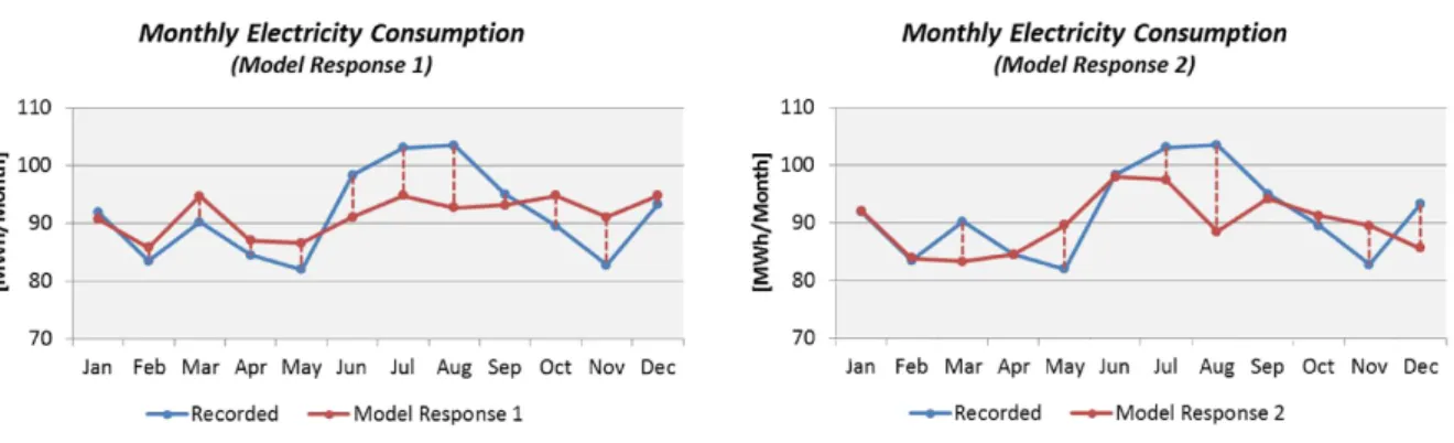
Figure 6 and Table 4 show the summary of adequacy of both model responses.
Figure 6 - Recorded and predicted whole building electricity consumption (monthly base)
Table 4 shows the statistical indexes summary at annual, monthly and hourly level. Table 4 - Statistical indexes summary
Index Model Response 1 Model Response 2 Reference
MBEyear,month,hourly -0.01% -1.8% <±5% (Waltz, 2000)
CV(RMSE)month 6.3% 6.8% <±15% (ASHRAE, 14)
Both models are able to predict annual and monthly electrical energy use and hourly power demand within the tolerance range listed in Table 4.
For model response 1 discrepancy comes from the fact of averaging profile which induces an underestimation of hourly consumption for the hottest months of the year (see June, July and August in Figure 6, left).
In the case of model response 2 the situation is different and the differences can be related to the incidence of weather conditions which are different than recorded data.
Finally, according to current criteria, is possible to conclude that both models have been
succesfully calibrated!
However, still some questions come to mind:
Now, we are sure about the accuracy reached when representing actual building energy performance, but; can we be sure about the accuracy when representing another different situation? Next sections
disccuss this issue in details.
Evaluating Model accuracy and its capability of measuring a new situation
Because, to evaluate proximity (point to point) of yearly two lists of 8760 values corresponds to a cumbersome analysis, it is needed to apply some complementary techniques such as statistical and visualization techniques.
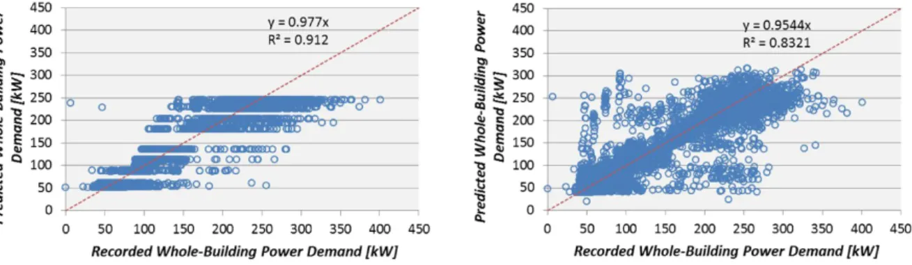
A curious aspect, which do not only occur when analyzing hourly results (Table 4), is the fact of obtaining more accurate results for the simple model (model response 1) instead of the detailed one (model response 2). In this part of the analysis is intended to find an explanation to this issue and also identify the capabilities and limitations of the information provided by statistical indexes. Figure 7 plots a comparison point by point between recorded and predicted data obtained from both models.
Figure 7 - Predicted versus recorded hourly power demand (Model Response 1 – left side; Model Response 2 – right side)
First of all, both graphs show a large dispersion between predicted and recorded data, even taking into account the good coeficient of determination ( ) obtained by both models, 0.91 and 0.83 respectively. The position of the points (above and under the red line) explain the “compensation error effect” that produced the low values obtained when index was evaluated (for all the time scales). ( ) index in annual and monthly base did not show big values mainly due to the capability of both models of predicting consumption in periods of time which do not change their conditions significantly from one scenario to another or from one year to another.
Where considerable differences were found was when evaluating ( ) in hourly time scale. For the case of model response 1 (which was built by means of averaged profiles) it makes sense because at some extreme conditions electrical consumption values can increase considerably, however in the case of model response 2 this issue is intriguing because it is supossely to be the most accurate model wich could be obtained.
The reason about this last issue is none other than the “desynchronization” between both profiles. It is impossible to replicate the same conditions for two equivalent days even if they correspond to the same date (in the case of two different years). This fact demonstrates that when evaluating calibration accuracy at small time scales (or scales where conditions are very variable) is not appropriate to make an analysis by comparing the proximity of two time series (point to point) but must be carry out another method that takes into account the dynamic behavior of the power demand, regardless its evolution over time.
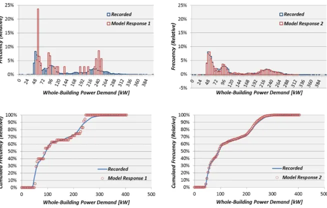
Figure 8 shows a bin analysis made over hourly consumption data. From a probabilistic point of view, it provides a distribution of power demand levels along the year. Predicted and recorded consumptions are plotted in terms of relative frequency and cumulated relative frequency.
Figure 8 - Relative and cumulated frequency comparison between recorded and predicted data (hourly base)
Now, differences between recorded and predicted data and the quality of both models responses are more evident. Model response 1 only providing 48 different hourly consumption values (24 for weekdays and 24 for weekends) spread all over the year is perhaps not enough for representing the real dynamic behavior of the electrical consumption.
On the other hand, model response 2 represents an incredibly accurate situation even taking into account the values obtained by evaluating the current criteria.
This approach certainly represents an appropriate way to evaluate accuracy in calibration procedures. Although until now, it has only provided visual comparison of two electrical profiles, it is imperative to define one or more indexes to quantify proximity between predicted and recorded data without using Euclidean distances.
Proposed Complementary Approach
The analysis carried out in the previous section highlighted the limitations of the current acceptance criteria and the necessity of going to more detailed timescales when determining accuracy and reliability of simulated data. In this section some complementary analyses are proposed to check reliability of the information provided by statistical indexes.
Operative hours
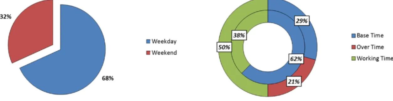
The comparison of corresponding hours to each day type and daily period, between simulated and recorded profiles is crucial to verify that the simulation was done according to reality. For example, year 2009 had in total 8760 hours (non leap year) divided in 5976 hours per weekday (249 days) and 2784 hours per weekend day (116 days).
Figure 9 – Annual operative time disaggregation according to daily period and day type. Corresponding to year 2009.
This issue was previewed when creating response profiles, so in this exercise, differences between simulated and recorded data come from modeling discrepancies and not from simulation ones.
Summary of hourly power demand by means of statistical plots
In real building operation, BEMS controls and allows the electrical use according to permanent daily periods (defined mainly according to occupancy). The occupants’ behavior and their decisions, the “calendar”, the effect of meteorological variables over thermal loads and over some BEMS decisions as well as the installed capacities of lighting, appliances and equipment determine the electrical power demand profile in terms of shape and order of magnitude.
Although this profile changes from one year to another or from one scenario to another there is a clear global behavior that can be revealed using the proper approach and tools.
Figure 10 shows a probabilistic approach plotting a (discrete) relative and its corresponding cumulated distribution for 3 year recorded data corresponding to DM28 building.
Figure 10 - DM28 relative frequency and cumulated frequency for whole building power demand. Recorded data for year 2008, 2009 and 2010.
A good agreement and a repeatable behavior are observed in both graphs plotted in Figure 10. Addressing the problem from a probabilistic point of view allows to identify the frequency of each event (consumption level) occurring during the year and also a way to evaluate calibration accuracy between two series of data.
In order to refine the results, this approach can be extended to different subsets of data grouped by: day type (week, weekends, holidays, etc.), daily periods (non-occupancy, working hours, etc.) and even could be associated to meteorological variables (temperature, humidity, etc.), in case of having reliable data.
Conclusions
In this paper, current criteria used to assess accuracy in building calibration procedures has been tested by means of two “simplified” models showing its strengths and weakness.
“Current criteria is necessary but not sufficient”
What current criteria do is: to compare predicted to recorded data point to point (calculating Euclidean distances) and estimating an average value which must be in accordance with a defined tolerance. This approach is appropriated when data integrated over a large period of time is analyzed. Annual and monthly consumption fit very well to be assessed by actual approach.
If a more detailed analysis is required another type of analysis is needed. Bin analysis has shown to be appropriate.
In the presence of a real calibration procedure, this same exercise (proposing a possible solution and evaluate its adequacy) can be used to determine the minimum requirements the model must fulfill in terms of accuracy. It would allow realizing whether the ultimate goal of the calibrated simulation model is reachable or not.
Finally, the building calibration problem will always remain an underdetermined mathematical problem and a unique solution is impossible to find, however the fact of having achieved replicating in a correct way the dynamic behavior of electrical consumption, suggests that the found solution is not far from the real one.
References
[1] Kaplan, M.B., McFerran, J., Jansen, J., Pratt, R. 1990. Reconciliation of a DOE2.1c model with monitored end-use data for a small office building. ASHRAE Transactions. 11 (1):981-993
[2] ASHRAE. 2002. ASHRAE Guideline: Measurement of energy and demand savings. ASHRAE Guideline 14-2002.
[3] US DOE. 2008. M&V Guidelines: Measurements and Verification for Federal Energy Projects, version 3.0
[4] Efficiency Valuation Organization. 2007. International Performance Measurement and Verification Protocol (IPMVP). Concepts and Options for Determining Energy and Water Savings – Volume 1.
[5] Reddy, T.A., Maor, I. 2006. Procedures for reconciling computer-calculated results with measured energy data. ASHRAE Research Project 1051-RP. Atlanta: American Society of Heating, Refrigerating and Air-Conditioning Engineers, Inc.
[6] Carroll, W.L., Hitchcock, R.J. 1993. Tuning Simulated Building Descriptions to match actual utility data: methods and implementation. ASHRAE Transactions, 99(y): 928-934.
[7] Reddy, T. (2011). Applied data analysis and modeling for energy engineers and scientists. [8] Bou-Saada, T.E.,Haberl, J. (1995). An improved procedure for developing calibrated hourly
simulation models. Proceedings of the 5th IBPSA Building Simulation Conference, Madison, Wisconsin, USA.
[9] Annex 53, Total Energy Use in Buildings: Analysis & Evaluation Methods, The International Energy Agency (IEA), www.ecbcsa53.org 2010.