Dataflow Modeling for Reconfigurable Signal Processing Systems

HAL Id: hal-01899410

https://hal.archives-ouvertes.fr/hal-01899410

Submitted on 19 Oct 2018

HAL is a multi-disciplinary open access

archive for the deposit and dissemination of

sci-entific research documents, whether they are

pub-lished or not. The documents may come from

teaching and research institutions in France or

abroad, or from public or private research centers.

L’archive ouverte pluridisciplinaire HAL, est

destinée au dépôt et à la diffusion de documents

scientifiques de niveau recherche, publiés ou non,

émanant des établissements d’enseignement et de

recherche français ou étrangers, des laboratoires

publics ou privés.

Dataflow Modeling for Reconfigurable Signal Processing

Systems

Karol Desnos, Francesca Palumbo

To cite this version:

Karol Desnos, Francesca Palumbo. Dataflow Modeling for Reconfigurable Signal Processing Systems.

Handbook of Signal Processing Systems, 3rd Edition, pp.787-824, 2019,

�10.1007/978-3-319-91734-4_22�. �hal-01899410�

Dataflow Modeling for Reconfigurable

Signal Processing Systems

Karol Desnos and Francesca Palumbo

Abstract Nowadays, adaptive signal processing systems have become a re-ality. Their development has been mainly driven by the need of satisfying di-verging constraints and changeable user needs, like resolution and throughput versus energy consumption. System runtime tuning, based on constraints/-conditions variations, can be effectively achieved by adopting reconfigurable computing infrastructures. These latter could be implemented either at the hardware or at the software level, but in any case their management and subsequent implementation is not trivial. In this chapter we present how dataflow models properties, as predictability and analyzability, can ease the development of reconfigurable signal processing systems, leading designers from modelling to physical system deployment.

1 Reconfigurable Signal Processing Systems

For many years, the design of a signal processing system was mostly driven by performance requirements. Hence, design effort was mainly focused on op-timizing the throughput and latency of the designed system, while satisfying constraints of reliability and quality of service, and minimizing the system production cost. In this context, a strong predictability of system behavior is essential, especially when designing safety-critical real-time systems. Many compile-time methodologies, computer-aided design tools, and static Models Karol Desnos

IETR, INSA Rennes, CNRS UMR 6164, UBL, Rennes, France e-mail: kdesnos@insa-rennes.fr

Francesca Palumbo

Universita degli Studi di Sassari, Italy e-mail: fpalumbo@uniss.it

of Computation (MoCs), such as the decidable dataflow MoCs [26], have been created to assist system designers in reaching these goals.

In recent years, the ever increasing complexity of signal processing sys-tems has lead to the emergence of new design challenges. In particular, mod-ern signal processing systems no longer offer a fixed throughput and latency, specifically tuned to satisfy all timing constraints in the most demanding scenarios from the system specification. Instead, modern systems must now dynamically adapt their behavior on-the-fly to satisfy strongly varying work-loads and performance objectives, while optimizing new design goals such as minimizing use of shared computational resources, or minimizing power con-sumption. These variations of the workload and performance objectives may be induced by functional and non-functional requirements of the system. An example of system with strongly varying functional requirements is the com-puting system managing a base station of the Long-Term Evolution (LTE) telecommunication network. Every millisecond, the bandwidth allocated for up to 100 active users connected to the managed antenna may change [50], with a strong impact on the amount and nature of computations performed by the system. An embedded video decoding system that lowers the quality of its output in order to augment battery life is an example of varying non-functional requirement [55, 48]. As presented in [64], increasing the dynamism of a signal processing often results in a partial loss of predictability, making it difficult, and sometimes impossible, to guarantee the real-time performance or the reliability (e.g. deadlock freedom) of a system.

The purpose of reconfigurable signal processing systems is to offer a care-fully balanced trade-off between system predictability and adaptivity. This trade-off between diverging properties is essential to meet classical constraints of system performance and reliability while satisfying varying requirements of modern system. To offer a trade-off between predictability and adaptivity, reconfigurable systems rely both on design-time analysis and optimization of system behavior, that make it possible to predict the system behavior, and on runtime management technique that enable system adaptation.

The objective of this chapter is to present how the analyzability of dataflow MoCs can be exploited to ease the development of reconfigurable signal pro-cessing systems. The chapter structure is briefly summarized as follows: Sec-tion 2 presents how reconfigurable systems can be efficiently modeled with dedicated dataflow MoCs, and Sections 3 and 4 presents how software and hardware techniques, respectively, can be used to implement reconfigurable applications efficiently. In more details, Section 2 formally introduces the concept of reconfigurable dataflow MoCs and discusses its key differences with decidable and dynamic classes of dataflow MoCs. This concept is il-lustrated through the semantics of several reconfigurable dataflow MoCs. In Section 3, software implementation techniques supporting the execution of reconfigurable dataflow application are presented. This section covers a wide range of software implementation techniques, spanning from compile-time op-timizations to runtime management system for reconfigurable applications.

Then, Section 4 presents a summary on reconfigurable computing systems, where both coarse grained and fine grained reconfiguration paradigm are ad-dressed describing how dataflow MoCs may help in mapping and managing this kind of highly flexible computing systems.

2 Reconfigurable Dataflow models

The high abstraction level of dataflow MoCs makes them popular models for specifying complex signal processing applications [26]. By exposing coarse-grain computational kernels1, the actors, and data dependencies between them, the First-In First-Out queues (Fifos), the dataflow semantics eases the specification of parallel applications, and provides necessary formalism for many verification and optimization techniques for the design of signal processing systems.

The expressiveness of a MoC defines the range of applications behavior this MoC can describe. The expressiveness of a dataflow MoC is directly related to its firing rules, which are used to specify how and when actors produce and consume data tokens on connected Fifos. Dataflow MoCs can be sorted into three classes depending on their expressiveness:

• Decidable dataflow MoCs [26]: all production and consumption rates are fixed at compile-time, either as fixed scalar, or with periodic variations. The key characteristics of decidable dataflow graphs is that, through an analysis of data rates, it is possible to derive a schedule of finite length at compile-time.

• Dynamic dataflow MoCs [64]: production and consumption rates can change non-deterministically at each actor firing, making these models Turing-complete ones. Hence, for most dynamic dataflow MoCs, schedula-bility, deadlock-freedom, real-time properties, and memory boundedness of application graphs can be verified neither at compile-time, nor at runtime. In some dynamic dataflow MoCs, this lack of analyzability is partially alleviated through specialization of the model semantics.

• Reconfigurable dataflow MoCs: production and consumption rates can be reconfigured (i.e. changed) non-deterministically at restricted points in application execution. These MoCs are sometimes also called paramet-ric dataflow MoCs [11]. This restparamet-riction limits the expressiveness of re-configurable dataflow models, but makes it possible to verify application properties, like schedulability, either at compile-time or at runtime, after a reconfiguration occurred.

1 _{Kernels are usually intended as subparts of an application providing a specific} compu-tation. In a perspective hardware implementation, the computationally intensive ones are the part of the application that are normally delegated to specific accelerators.

The following subsections formally introduce the reconfiguration semantics behind reconfigurable dataflow MoCs, and shows how it benefits model ana-lyzability through the presentation of several reconfigurable dataflow MoCs. Implementation optimization techniques taking advantage of the reconfigu-ration semantics are presented in Section 3 and 4.

2.1 Reconfiguration Semantics

The reconfiguration semantics behind reconfigurable dataflow MoCs is a mathematical model that makes it possible to detect potentially unsafe re-configurations of an application graph [44]. A reconfiguration is said to be unsafe if it may result in an unwanted and undetected state of the applica-tion, such as a deadlock or an inconsistence in production and consumption rates.

The reconfiguration semantics for dataflow MoCs is based on the defini-tion of hierarchical actors, parameters, and quiescent points. The reconfig-uration semantics can be implemented by any dataflow MoC with atomic actor firings. This assumption guarantees the applicability of the reconfigu-ration semantics to a broad range of dataflow MoCs, including decidable [26], multi-dimensional [33], and some dynamic dataflow MoCs [64].

Formally, a hierarchical graph is defined as a set of actors A. An actor a ∈ A can either be an atomic actor, an actor whose internal behavior is specified with host code, or a hierarchical actor, an actor whose internal be-havior is specified with a subset of actors Aa⊂ A. The top-level graph itself

is considered as a hierarchical actor with no parent, and that contains all other actors in A. Each actor a is associated to a dedicated set of parameters Pa, that can influence both its production and consumption rates, and the

computations it performs. At any point in execution time, each parameter

p ∈ P (= S

a∈APa) is associated to a value given by a valuation function:

val (p) whose type (e.g. integer, real, boolean, ...) depends on the underly-ing model semantics. The value val (p) of a parameter may be independent, or may depend on the value of one or several other parameters in P . The transitive relation q depends on p, between two parameters p 6= q, is noted p q. Reconfiguration occurs when the value of an independent parameter is modified during the execution of the application.

Figure 1 shows an example of graph specified with a synthetic dataflow MoC implementing the reconfiguration semantics. Figure 1a illustrates the semantics, which is then used to build up the example in Figure 1b. The graph of Figure 1b consists of 5 actors, including one hierarchical actor h that contains two atomic actors C and D. Each consumption and production rate is defined by a dedicated parameter whose valuation function is specified as an expression written next to the graph. In this graph, p, s, and t are

independent parameters and all other parameters have dependencies; as for example p r. FIFO Hierarchical actor Atomic actor A Port and rate y h (a) Semantics.

A

p q

h

v w

B

s t u r

C

D

p:= 6 q:= p/2 r:= q t:= 2 s:= 4 u:= t v:= s w:= 2*t (b) Graph and current valuation of parameters. Fig. 1 Synthetic dataflow MoC implementing the reconfiguration semantics.

Reconfiguration semantics models as a quiescent point the state of an actor between two firings. Like actor firings, the set of quiescent points Qa

of an actor a is ordered in time according to a transitive precedence relation. Since firings of actors contained in a hierarchical subgraph cannot span over multiple firings of their enclosing actor, when a hierarchical actor is quiescent, all actors contained in its hierarchy must also be. A graphical representation of quiescent points for the graph of Figure 1 is presented in Figure 2.

Top-level A h B C D

Fig. 2 Abstract representation of the quiescent points for the graph of Figure 1. Vertical lines represent quiescent points of actors. Dotpoint arrows represent actor firings and define a partial ordering of quiescent points.

The reconfiguration semantics requires reconfigurations of any indepen-dent parameter p ∈ P to happen only during a quiescent points q ∈ Q(= S

a∈AQa) at execution time. The set of parameters reconfigured during a

quiescent point q is noted: R(q) ⊆ P .

When using a dataflow MoC implementing the reconfiguration semantics, a compile-time analysis of parameters and quiescent points of an application graph can be used to verify model-specific reconfiguration safety require-ments [44]. Safety requirerequire-ments of a dataflow MoC are expressed as state-ments in the form “Parameter p is constant over firings of actor a”. Formally: Definition 1. Parameter p is constant over firings of actor c if and only if ∀a ∈ A, ∀q ∈ Qa, ∀r ∈ R(q), r p ⇒ q ∈ Qc.

For example, in the Synchronous Dataflow (SDF) MoC, decidability can be expressed as the following safety requirement: all parameters are required to be constant over firings of the top-level actor.

In [11], Bouakaz et al. present a Survey of dataflow MoCs adopting the reconfiguration semantics. Next sections present examples of MoCs imple-menting the reconfiguration semantics.

2.2 Reconfigurable dataflow models

2.2.1 Hierarchy-based Reconfigurable Dataflow Meta-Models The purpose of a dataflow meta-model is to bring new elements to the seman-tics of a base dataflow MoC in order to increase its modeling capabilities. The Parameterized and Interfaced Dataflow Meta-Model (PiMM) [17] and Param-eterized Dataflow [8] are two dataflow meta-models with similar purpose: bring hierarchical graph composition and safe reconfiguration features to any decidable dataflow MoC that has a well-defined notion of graph iteration and repetition vector, such as SDF and Cyclo-Static Dataflow (CSDF) [26], or Multi-Dimensional SDF (MDSDF) [33]. A base dataflow MoC whose seman-tics is enriched with PiMM or with the parameterized dataflow meta-model is renamed with prefixes

π

- and P-, respectively. For example, Parameter-ized and Interfaced SDF (

π

SDF) and Parameterized SDF (PSDF) are the reconfigurable generalizations of the decidable SDF MoC.

In PiMM and parameterized dataflow meta-models, safe reconfiguration is expressed as a local synchrony requirement [8]. Intuitively, local synchrony requires the repetition vector of the subgraph of a hierarchical actor to be configured at the beginning of the execution of this subgraph, and to remain constant throughout a complete graph iteration, corresponding to a firing of the parent actor. Hence, in locally synchronous hierarchical subgraph, all parameters influencing production and consumption rates of actors must re-main constant over the firing of their parent actor. Formally, with Sc, the set

of direct child actors of a hierarchical actor c ∈ A, where direct child means that ∀h ∈ Sc, d ∈ Sh⇒ d /∈ Sc.

Definition 2. Subgraph Sc of actor c ∈ A, is locally synchronous if and only

if: ∀a ∈ Sc, ∀p ∈ Pa, the requirement “p is constant over firings of c” is

verified.

The semantics of PiMM, which is an evolution of the parameterized dataflow semantics, is illustrated in Figure 3. An example of

π

SDF graph is given in Figure 4.

In PiMM, graph compositionality is supported by hierarchical actors, as defined in the reconfiguration semantics, and by data interfaces. The purpose of interface-based hierarchy [52] is to insulate the nested levels of hierarchy in

PiMM semantics

Configuration input interface Configuration input port Locally static parameter Parameter dependency P Parameterization semantics Configuration output port Configurable parameter Configuration actor P

A

Reconfiguration semantics Delay and number of tokens FIFO Actor

A

Port and rate 3 x4 SDF

semantics Hierarchysemantics

Data input interface Data output interface Hierarchical actor out in

h

Fig. 3 Semantics of the Parameterized and Interfaced Dataflow Meta-Model (PiMM).

terms of graph consistence analysis. To do so, data interfaces automatically duplicate and discard data tokens if, during a subgraph iteration, the number of tokens exchanged on Fifos connected to interfaces is greater than the number of token produced on the corresponding data ports of the parent actor. Converge Channel Decoding max CBsPerUE NbUE Config NbUE mac symbols Converge KeepCurrent Tones Config NbCB NbCB symbols PerUE

Process. Process.Bit TurboDec. CheckCRC

sink sink NbCB maxCBsPerUE NbCB 1 1 1 NbCB 1 1 MaxCBsPerUE*NbUE MaxCBsPerUE 1 NbUE 1 1 1

Fig. 4 Example of

π

SDF graph. Bit processing algorithm of the Physical Uplink Shared Channel (PUSCH) decoding of the LTE telecommunication standard [17].

The parameterization semantics of PiMM consists of parameters and pa-rameter dependencies as new graph elements, and configuration input ports and interfaces as new actor attributes. The value associated to a parameter of a graph is propagated through explicit parameter dependencies to other parameters and to actors. In the

π

SDF MoC, it is possible to disable all firings of an actor by setting all its production and consumption rates to zero. As illustrated in Figure 4, parameter values can be propagated through multiple levels of hierarchy using a configuration input port on a

hierarchi-cal actor and a corresponding configuration input interface in the associated subgraph.

The reconfiguration semantics of PiMM is based on actors with special firing rules, called configuration actors. When fired, reconfiguration actors are the only actors allowed to dynamically change the value of a parameter in their graph. As a counterpart for this special ability, reconfiguration actors must be fired exactly once per firing of their parent actor, before any non-configuration actor of their subgraph. This restriction is essential to ensure the safe reconfiguration of the subgraph to which configuration actors belong. To be strictly compliant with Definition 2, configuration actors and other actors of a subgraph can be considered as two separate subgraphs, executed one after the other.

The local synchrony requirement of the

π

SDF MoC naturally enforces the predictability of the model. After firing all configuration actors of a subgraph, all parameters values, and hence all actor production and consumption rates of this subgraph, are known and will remain fixed for a complete subgraph iteration. Runtime analyses and optimization techniques can be used to com-pute the repetition vector of the subgraph, to optimize the mapping and scheduling of actors, to allocate the memory, or to verify that future real-time deadlines will be met. An important benefit of this predictability is the support for data-parallelism which is often lost in dynamic dataflow MoCs. Data parallelism consists in starting several firings of the same actor in par-allel if enough data tokens are available. Data-parpar-allelism is supported only if the next sequence of firing rates is know a priori, as is the case in

π

SDF graphs. In dynamic dataflow MoCs [64], the firing rules of an actor generally depend on its internal state after completion of its previous firing. This inter-nal dependency between actor firings forces their sequential execution, thus preventing data parallelism.

Figure 4 presents a

π

SDF specification of the bit processing algorithm of the Physical Uplink Shared Channel (PUSCH) decoding which is part of the LTE telecommunication standard. The LTE PUSCH decoding is executed in the physical layer of an LTE base station (eNodeB). It consists of receiv-ing multiplexed data from several User Equipments (UEs), decodreceiv-ing it and transmitting it to upper layers of the LTE standard. Because the number of UEs connected to an eNodeB and the rate for each UE can change every millisecond, the bit processing of PUSCH decoding is inherently dynamic and cannot be modeled with static MoCs such as SDF. Further details on this application, and specification using the parameterized dataflow meta-model, can be found in [50]

Compile-time and light-weight runtime scheduling technique for executing

π

SDF and PSDF graphs, are presented in Section 3. Combination of the parameterized dataflow semantics and the CSDF MoC is studied in [32] for the design of software-defined radio applications.

2.2.2 Statically Analyzable Reconfigurable Dataflow Models Schedulable Parametric Dataflow (SPDF) and Boolean Parametric Dataflow (BPDF) are non-hierarchical reconfigurable generalizations of the SDF MoC that emphasize static model analyzability. In particular, the semantics of the SPDF and BPDF MoCs make it possible to verify safe reconfiguration re-quirements and to guarantee graph consistency and liveness at compile time. In

π

SDF and PSDF, although local synchrony can be checked at compile time, consistency and liveness of a subgraph can only be verified at runtime, after configuration of all the parameters contained in this subgraph.

3 2p 1 1

B

C

set q[2p] set p[1]

A

F

q 2pq 1 1

D

E

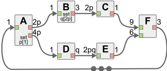
4p 2p 6 9 3 1

Fig. 5 Example of Schedulable Parametric Dataflow (SPDF) graph.

In the SPDF MoC semantics, symbolic parameters P with integer values in N∗are used for parameterization. Special actors, called modifiers, have the ability to dynamically change the value of a symbolic parameter. To ensure safe reconfiguration, a modifier m ∈ A will set a new value for a parameter p ∈ P with a pre-defined change period α ∈ N∗_{. In practice, this means}

that the value of p will be changed every α firings of m. In an SPDF graph, as shown in Figure 5, the annotation “set p[α]” is used to denote that an actor is a modifier of parameter p, with change period α. Change periods, and production and consumption rates of actors are specified with products Qn

i=0ei, where ei is either an integer in N

∗_{, or a symbolic parameter p ∈ P .}

Using balance equations of actor production and consumption rates, simi-lar to those used for SDF graphs [26], graph consistency can be verified, and a symbolic repetition vector can be computed. The basic operation used to find the symbolic repetition vector of an SPDF graph is the computation of the Greatest Common Divisor (GCD) of the numbers of data tokens produced and consumed on each Fifo of the graph. Using this GCD, the numbers of repetition of the producer and consumer actors, relatively to each other, can be deducted by dividing the rates of the actors by this GCD. For ex-ample, in the graph of Figure 5, the GCD of the Fifo between actor D and E is gcdDE = gcd(q, 2pq) = q, which means that actor E will be executed

rateD/gcdDE= 2pq/q = 2p times for each rateE/gcdDE= q/q = 1 execution

of actor D. Using this principle, an algorithm detailed in [22] can be used to compute the parametric number of repetition of all actors in an SPDF

graph. Using this algorithm on the SPDF graph of Figure 5, the following symbolic repetition vector is obtained: A3_B6p_C9_D12p_E6_{F , where X}a _means

that actor X is fired a times per iteration of the graph. Notation #X is used to denote the repetition count of an actor X ∈ A. Similarly, liveness (i.e. deadlock-freedom) of graphs can be verified statically with an analysis of cyclic data-paths inspired from SDF graph techniques.

Reconfiguration safety in SPDF graphs is based on the notion of parameter influence region. The influence region R(x) of a parameter x is the set of: a) Fifos whose rates depend on x, b) actors connected to these Fifos, and c) actors whose numbers of repetitions depend on x. For example in Figure 5, R(q) comprises Fifo DE and actors D and E; and R(p) comprises the whole graph except actor F and Fifos connected to it.

Two safe reconfiguration requirements are used in SPDF: data and period safety. Intuitively, data safety requires that the region R(p) influenced by a parameter p ∈ P comes back to an initial state, in terms of the number of data-tokens on Fifos, between each reconfiguration of p. In other words, data safety requires the (virtual) subgraph composed by R(p) to complete a kind of local iteration and be quiescent when a reconfiguration of a parameters in-fluencing it occurs. Formally, data safety requires that ∀p ∈ P , with modifier m ∈ A and change period α, all actors a ∈ R(p) have a repetition count #a such that gcd (#a, #m/α) = #m/α (i.e. #a is a multiple of #m/α). For ex-ample in Figure 5, with actor E ∈ R(q) and modifier B annotated “set q[2p]”, actor E is data safe since #E = 6 is a multiple of #B/2p = 6p/2p = 3.

Period safety restricts how often a parameter q can be reconfigured by its modifier m if #m itself depends on a parameter p. In this case, period safety ensures that q is reconfigured at least as often as the start of a new iteration of the subgraph formed by R(p). Formally, ∀p, q ∈ P with modifiers mpand mq, change period αpand αq, and #mqdepending on p, period safety

requires #mq/αq to be a multiple of #mp/αp. If this condition is not met,

reconfiguration of q may happen in the middle of an iteration of the subgraph formed by R(p), when it is not quiescent. For example, in Figure 5, repetition count #B = 6p of the emitter of q depends on p, but its change period is safe since #B/2p = 3 is a multiple of #A/1 = 3. With the period of q set to 3p instead, the graph would remain data safe but would no longer be period safe, as #B/3p = 2 is not a multiple of #A/1 = 3. A consistent, data and period safe SPDF graph will always be schedulable in bounded memory [22]. The semantics of the BPDF MoC is closely related to the one of the SPDF MoC, and provides the same advantages in terms of static graph analyzabil-ity [6]. The main difference between the two MoCs is that reconfigurable integer parameters of SPDF are replaced with reconfigurable boolean pa-rameters in BPDF. Through combinational logic expressions, these boolean parameters are used to change the BPDF graph topology, by enabling and disabling Fifos. This feature is equivalent to setting data rates to 0 in the

Examples of SPDF and BPDF graphs of multimedia, signal processing, and software defined radio applications can be found in [6, 16, 22]. Compilation techniques for deploying SPDF graphs onto multi and many-core architecture will be presented in Section 3.

2.3 Dynamic Dataflow MoCs and Reconfigurability

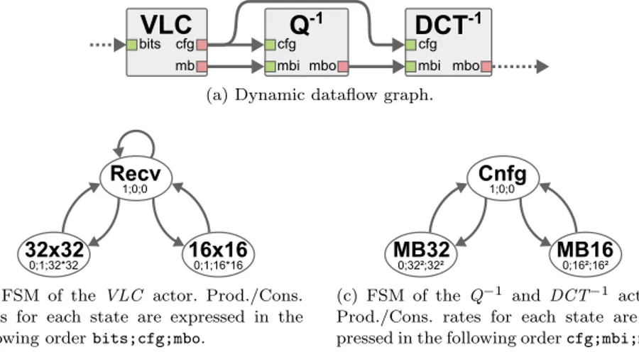
In dynamic dataflow MoCs, as presented in [64], production and consumption rates of actors may change dynamically at each firing, depending on the firing rules specified for each actor. In most dynamic dataflow MoCs, the semantics include elements to specify explicitly the internal firing rules of each actor. A common way to characterize firing rules of a dynamic actor is to model its internal state with a Finite State Machine (FSM), or a similar model like a Markov chain, and to associate each FSM state with pre-defined production and consumption rates for each data port. These FSMs can be specified either explicitly by the application designer, using a dedicated language, as in the Scenario-Aware Dataflow (SADF) and Core-Functional Dataflow (CFDF) MoCs [40, 64], or implicitly in the language describing the internal behavior of actors, as in frameworks based on the CAL Actor Language (CAL) [13, 21, 67].

An example of dynamic dataflow graph with associated FSMs is presented in Figure 6. This graph represents the residual decoding of macro-blocs of pixels in a video decoding application. The semantics used for the FSMs presented in Figures 6b and 6c is similar to the one of the CFDF MoC. Each state of the FSMs is associated with an integer production and consumption rate for each port of the corresponding actor. When enough data tokens are available on the input Fifos according to the current actor state, the actor is fired and one state transition is traversed, thus deciding the next firing rule. In the graph of Figure 6, the Variable Length Code (VLC ) actor is re-sponsible for decoding the information corresponding to each macroblock (i.e. square of pixel) from the input bitstream. To do so, the VLC actor reads the input bitstream bit-by-bit in the Recv state, and fills an internal buffer. When enough bits have been received, the VLC actor detects it, and goes to the 16x16 or 32x32 state, depending on the dynamically detected macroblock size. In the 16x16 or 32x32 states, the VLC actor produces a configuration data-tokens on its cfg port, and quantized macroblock coefficients on its mb port. The configuration data-token is received by the dequantizer actor Q−1 and the inverse discrete cosine transform actor DCT−1, which successively process the quantized macroblock coefficients in the state corresponding to the dynamically detected macroblock size: 16x16 or 32x32.

Although dynamic dataflow MoCs inherently lack the predictability that characterize reconfigurable dataflow MoCs, several techniques make it pos-sible to increase the predictability of a dynamic dataflow graph in order to

enable a reconfigurable behavior. The common point between these tech-niques, is that they exploit the actor behavioral information specified with FSMs in order to make parts of the application reconfigurable. Two different approaches are presented hereafter: in Section 2.3.1 classification techniques are used to identify reconfigurable behavior in application graphs specified with existing dynamic MoCs, and in Section 2.3.2, semantics of dynamic dataflow MoCs is extended to ease specification of reconfigurable behavior within dynamic applications. Further hardware reconfigurable implementa-tion techniques based on dynamic dataflow MoCs are introduced in Secimplementa-tion 4.

2.3.1 Classification of Dynamic Dataflow Graphs

The basic principle of classification techniques for dynamic dataflow graphs is to analyze the internal FSM of one or more actors in order to identify patterns that correspond to statically decidable behaviors. Here, a pattern designates a sequence of firings of one or more actors that, when started, will always be executed deterministically when running the application, despite the theoretical non-deterministic dynamism of the dataflow MoC.

VLC

Q

-1

_DCT

-1

cfg mb

bits cfg cfg

mbi mbo mbi mbo

(a) Dynamic dataflow graph.

32x32

0;1;32*32 16x160;1;16*16 Recv

1;0;0

(b) FSM of the VLC actor. Prod./Cons. rates for each state are expressed in the following order bits;cfg;mbo.

MB32

0;32²;32² MB160;16²;16² Cnfg

1;0;0

(c) FSM of the Q−1 _{and DCT}−1 _actors. Prod./Cons. rates for each state are ex-pressed in the following order cfg;mbi;mbo. Fig. 6 Dynamic dataflow graph inspired by the residual decoding of a video decoder.

In the example of Figure 6, an analysis technique can detect two sequences of actor firings, corresponding to the processing of a macroblock of size 16x16 and 32x32, respectively. The first sequence is triggered when the VLC actor fires in the 16x16 state, which will always be followed by two firings of each of the Q−1 and DCT−1 actors, in the Cnfg and MB16 states. The second sequence is similar for the 32x32 configuration.

In [13], Boutellier et al. propose a technique to analyze a network of ac-tors specified with CAL, and detect static sequences of actor firings in their

FSMs. Once detected, each alternative sequence of actor firings is transformed into an equivalent SDF subgraph. Similarly to what is done in reconfigurable dataflow MoCs, SDF subgraphs are connected using switch/select actors ca-pable of triggering dynamically an iteration of a selected SDF subgraph. As shown in [13], application performance can be substantially improved by exploiting the predictability of SDF subgraphs to decrease the overhead of dynamic scheduling of actor firings.

In [21], Ersfolk et al. introduce a technique to characterize dynamic actor by identifying the control tokens of the application. A control token is defined as a data token whose value is used in actor code to dynamically decide which firing rule will be validated for the next actor firing. For example, in Figure 6, the data tokens exchanged on the cfg ports are control tokens, as they decide the next firing rules for the Q−1 and DCT−1 actors. Once a control token is identified, the data and control path influencing its value is backtracked both through graph Fifos and by applying an instruction-level dependency analysis to actor CAL code. By analyzing the datapath of control tokens, complex relations between firing rules of different actors can be revealed. As in the previous technique, these relations between firing rules of dynamic actors can be exploited to transform some part of a dynamic dataflow graph into an equivalent reconfigurable graph.

There exist several other techniques whose purpose is to detect recon-figurable or static behavior from a dynamic dataflow description. In [67], a set of rules are specified to classify the behavior of individual actors as static, cyclo-static, quasi-static, time-dependent (i.e. non-deterministic), and dynamic. These rules can be verified either by analyzing the firing rules of an actor, or by using abstract interpretation which allows verifying these rules for all possible actor states [67]. In [20], another technique based on model-checking is used to detect statically schedulable actions in a dynamic dataflow graph.

2.3.2 Reconfigurable Semantics for Dynamic Dataflow MoC Parameterized Set of Modes (PSM) is an extension of the CFDF MoC which brings parameterization semantics on top of the dynamic semantics of the CFDF model [40]. The purpose of the PSM-CFDF MoC is to improve the analyzability of FSMs in a network of actors by explicitly specifying graph-level parameters that influence the dynamic dataflow behavior of one or more actors.

In the PSM-CFDF semantics, an actor a ∈ A is associated to an FSM where each state, called a mode, corresponds to a fixed consumption and production rate. The set of all modes of an actor a is noted Ma. Each time

a mode ma∈ Ma of an actor a is fired, it selects the mode that will be used

for the next firing of a. The mode selected for the next firing of an actor a depends on the parameter values, called a configuration, of a set of parameters

P aram(a) specified at graph-level. The set of all valid configurations for an actor a is noted DOMAIN (a)

Figure 7 presents an example of PSM-CFDF graph modeling part of the Orthogonal Frequency-Division Multiplexing (OFDM) demodulation of an LTE receiver, inspired by [16, 50]. Parameter M takes value in {1, 2} and is used to switch the application behavior between a low-power mode M = 1, where a 5MHz bandwidth is received with QPSK modulation, and a high-throughput mode M = 2, where a 10MHz bandwidth is received with 16QAM modulation. Parameter B takes integer values between 1 and Bmax_{, and is}

used to control the vectorization of computation, i.e. the number of data tokens buffered in order to be processed in a single firing of actors. In low-power mode (resp. high-throughput mode), the FFT actor processes 512 (resp. 1024) samples and outputs symbols for 300 (resp. 600) subcarriers, each of which is then decoded by the Demap actor, using QPSK (resp. 16QAM) modulation, and producing 600 (resp. 2400) bits of data. As presented in Figures 7b and 7c, the fully connected FSMs of the two actors each contain 2 ∗ Bmax_modes. 512MB

FFT

300MB B

Demap

2MB (a) PSM-CFDF graph 5MHz M=1,B=2 10MHzM=2,B=2 5MHz M=1,B=1 10MHzM=2,B=1 5MHz M=1,B=Bmax 10MHz_M=2,B=Bmax (b) Partial FSM of the FFT actor.

QPSK

M=1,B=2 16QAMM=2,B=2 QPSK

M=1,B=1 16QAMM=2,B=1

QPSK

M=1,B=Bmax 16QAM_M=2,B=Bmax (c) Partial FSM of the Demap actor. Fig. 7 PSM-CFDF graph of an OFDM demodulator used in LTE standard [16, 40, 50].

Building on the graph-level parameterization semantics, the basic idea of PSM-CFDF is to gather actor modes into groups of modes with similar prop-erties (e.g. dataflow rates, mapping, ...) for a subsequent analysis or optimiza-tion of the applicaoptimiza-tion. These groups of modes are called the Parameterized Set of Modes (PSM) of an actor. Formally, a PSM of an actor a is defined as ρ = (S, C, f ), where S ⊂ Ma is a subset of the modes of a, C ⊂ DOMAIN (a)

is a subset of the configurations of a, and f : C → S is a function giving the current mode in S depending on the current configuration in C. The set of all PSMs of an actor a, noted PSM (a), must cover all modes of a; for-mally S

transition graph, whose vertices are the PSMs of the actor, and whose edges represent possible transitions from a PSM to another, as originally specified in the actor FSM.

PSMs of an actor can be specified explicitly by the application developer, but can also be deduced automatically from an analysis of the parameterized PSM-CFDF graph, or from execution traces [40]. Figure 8 presents the tran-sition graph created for the FSMs in Figures 7b and 7c, assuming that values of parameters B and M are changed simultaneously when no data-token is present on Fifos of the graph of Figure 7. This transition graph contains two PSMs ρ1 and ρ2, gathering modes for M = 1 and M = 2 respectively.

ρ1

M=1,B=1..Bmax

ρ2

M=2,B=1..Bmax Fig. 8 Transition graph for the PSM-CFDF actors of Figure 7.

A smart grouping of actor modes into PSMs can be used to produce a transition graph where each PSM corresponds to a static schedule of actor firings [40, 54]. For example in Figure 8, each of the two PSMs corresponds to a static scheduling of the PSM-CFDF graph, with FFT1Demap300for ρ1, and FFT1Demap600for ρ2, regardless of the value of parameter B. In such a case, changing the active PSM triggers a reconfiguration of the application that switches between pre-computed static schedules, which considerably reduces the workload of the application scheduler.

Smart PSM grouping can efficiently address many optimization objectives, such as maximizing application performance on heterogeneous platforms [40], or minimizing the allocated memory footprint for the execution of a dynamic graph [54].

3 Software Implementation Techniques for

Reconfigurable Dataflow Specifications

As shown in previous section, dataflow MoCs can efficiently capture the coarse-grain reconfigurable behavior of a signal processing system. From the dataflow perspective, a reconfigurable behavior can be modeled as an explicit lightweight control-flow enabling predictable and possibly parameterized se-quences of actor firings. A reconfigurable dataflow behavior can either be explicitly specified by the system developer using specialized dataflow MoCs, or be extracted automatically from a more dynamic system specification.

To execute a dataflow graph, a set of techniques must be developed to implement the theoretical MoC semantics and execution rules within diverse hardware and software environments. Implementation techniques are

com-monly responsible for mapping and scheduling actor firings onto available processing elements and for allocating memory and communication resources. Depending on the predictability of the implemented dataflow MoC, these im-plementation techniques can be part of the compilation process, or part of a runtime manager or operating system [37].

This section presents a set of software implementation techniques for dataflow specifications that exhibit a reconfigurable behavior. By taking ad-vantage of the reconfigurable behavior of applications, the presented tech-niques optimize systems in terms of performance, resource usage, or energy footprint. Implementation techniques responsible for translating dataflow specifications with reconfigurable behavior into synthesizable hardware im-plementations are presented in Section 4. A more general description of soft-ware compilation techniques for other parallel programming models is pre-sented in Chapter [39].

3.1 Compile-time Parameterized Quasi-Static

Scheduling

In general, dynamic and reconfigurable dataflow MoCs are non-decidable models. Hence, contrary to decidable dataflow MoCs [26], it is not possible to determine at compile time a fixed sequence of actor firings (i.e. a schedule) that will be repeated indefinitely to execute a reconfigurable dataflow graph. A quasi-static schedule of a dataflow graph, is a schedule where as many scheduling decisions as possible are made at compile time and only a few data-dependent decisions are left for the runtime manager. The purpose of quasi-static scheduling is generally to increase application performance by relieving the runtime manager from most of its scheduling computations overhead [9, 12].

In practice, a quasi-static schedule derived from a dataflow graph with a re-configurable behavior is expressed as a parameterized looped schedule [9, 35]. Formally, a parameterized looped schedule S is noted S = (I1I2...In)λwhere

λ is an integer repetition count whose expression may depend on parame-ter values, and instruction Ii represents either the firing of an actor a ∈ A,

or a nested parameterized looped schedule. The set of instructions I1I2...In

of a parameterized looped schedule S is called the body of S. For example, A(B(CD)2_E)p_{is a parameterized loop schedule with two nested loops, where}

actor A is executed once, followed by p executions of the sequence of actor firings (BCDCDE). A quasi-schedule is valid only if all loop iteration counts remain constant throughout firing of their associated body. When building a quasi-static schedule from a reconfigurable dataflow graph, validity of the schedule is usually enforced by the safe reconfiguration requirement of the dataflow graph (see Section 2.1).

i A a b B o (a) Original pair of actors.

g = gcd(a, b) x = i × (b/g) y = o×(a/g) (b) Equations. x G y (c) Resulting actor. r e p e a t b/g t i m e s{ f i r e A; } r e p e a t a/g t i m e s{ f i r e B; } (d) Pseudo-code for G. Fig. 9 Basic grouping operation used to build a quasi-static schedule.

An algorithm to build a quasi-static schedule from a PSDF (or

π

SDF) graph is given in [9]. This algorithm, called Parameterized Acyclic Pairwise Grouping of Adjacent Nodes (P-AGPAN), is an extension of a scheduling algorithm for SDF graphs whose purpose is to build a schedule minimizing both code size and memory footprint allocated for Fifos. The basic opera-tion of the P-AGPAN algorithm, illustrated in Figure 9, is to select a pair of actors connected with a Fifo, and to replace them with a composite actor whose internal behavior is defined with a parameterized looped schedule. For example, the pair of actors A and B from the graph of Figure 9a can be replaced with the composite actor G presented in Figure 9c. Using equations from Figure 9b, the internal behavior of actor G can be represented with the following parameterized looped schedule: Ab/g_Ba/g_{. Pseudo-code}

corre-sponding to the internal behavior of the composite actor G is presented in Figure 9d.

Applying the P-AGPAN algorithm to a PSDF or a

π

SDF (sub)graph consists of iteratively selecting a pair of actors and applying the pairwise grouping operation, until all actors of the considered subgraph are merged. The order in which pair of actors are selected for grouping influences code size and memory requirements of the generated quasi-static schedule. To minimize code size and memory requirements [9], priority is given to actor pairs connected with:

1. a single-rate Fifo (i.e. a Fifo with equal but possibly parameterized pro-duction and consumption rates),

2. a Fifo associated to constant rates,

3. a Fifo associated with parameterized rates whose gcd can be computed statically.

If a subgraph contains non-connected actors, as is the case with configuration actors and other actors of a

π

SDF graph, then these actors are added to the quasi-static schedule in the execution order imposed by the execution rules of the MoC. The P-AGPAN algorithm is applied in a bottom-up approach to all subgraphs of an application, starting from the innermost subgraph up to the top-level graph.

Figure 10 illustrates the application of the P-AGPAN algorithm to the LTE

π

SDF graph from Figure 4. Figure 10a presents a simplified version of the

π

SDF graph with 1-letter actor and parameter names. Figure 10c

A M B 1 v 1 h 1 Mv M C w D 1 1 M w w E 1 1 F 1 1 G 1 w I 1 v

(a) Simplified

π

SDF graph with 1-letter actor names.

/* top - l e v e l g r a p h */ f i r e A; // S e t s v f i r e B; r e p e a t v t i m e s{ /* h */ f i r e C; // S e t s w r e p e a t w t i m e s{ f i r e D; f i r e E; f i r e F; f i r e G; } f i r e I; } (b) Quasi-static pseudo-code

Grouped actor pair: Schedule: Simplified schedule:

1. D & E → D1_E1 _{→ DE}

2. F & G → F1_G1 _{→ F G}

3. (DE) & (F G) → (DE)1_{(F G)}1 _{→ DEF G}

4. (DEF G) & I → (DEF G)w_I1 _{→ (DEF G)}w_I

5. C & ((DEF GI)w_{I) → C}1_{((DEF GI)}w_I)1_{→ C(DEF GI)}w_{I = h}

6. B & h → B1_hv _{→ Bh}v _{= B(C(DEF GI)}w_I)v

7. A & Bhv _{→ A}1_(Bhv₎1 _{→ ABh}v _{= AB(C(DEF GI)}w_I)v

(c) Step-by-step construction of the quasi-static schedule using algorithm from [9]. Fig. 10 Quasi-static scheduling for the LTE

π

SDF graph of Figure 4

details the step-by-step execution of the P-AGPAN algorithm for this

π

SDF graph. The first column of Figure 10c presents the pair of actors selected for grouping at each step, the second column presents the internal parameterized looped schedule of the resulting composite actor, and the last column present the same schedule with simplified notations. Steps 1 to 5 correspond to the application of the P-AGPAN algorithm to the hierarchical subgraph of actor h, and steps 6 and 7 to the top-level graph. The pseudo-code corresponding to the quasi-static schedule AB(C(DEF GI)wI)v is presented in Figure 10b. An algorithm for building a quasi-static schedule for a SPDF graph is given in [22]. Briefly, this algorithm first consists of computing the symbolic repetition vector of an SPDF graph, and then finding an ordering of all pa-rameters pisuch that #M (p_α(p i+1)

i+1) = fi·

#M (pi)

α(pi) , where: #M (pi) is the repetition

count of the emitter of pi, α(pi) is its change period, and, finally, fi a

para-metric expression. Once this order is established, the quasi-static schedule is obtained by ignoring Fifos with delays, and constructing a schedule of ac-tors in topological order, where each actor X is written: (((XfN +10 ₎f

0 N_)...)f

0 1_,

where f0

i are expressions depending on the N parameters used and modified

by X [22]. In the constructed quasi-static schedule, which is not a param-eterized loop schedule, each parenthesis corresponds to a new value of the parameters used or set by the actor. For example, the quasi-static schedule for the SPDF graph of Figure 5 with explicit set and get of parameter values is

(A; set p)3_{(get p; (B}2p_{; set q))}3_{(get p; C}3₎3_{(get p; (get q; D}4p₎₎3_{(get p; (get q;}

E2₎₎3_{F (where all} 1 _{exponent were omitted). An equivalent parameterized}

looped schedule can be obtained by factorizing parenthesis with equivalent exponents and matching set/get: ((AB2p_C3_(D4p_E2₎₎3_{F .}

Further works on quasi-static scheduling include a technique for dynamic dataflow graphs that exhibit reconfigurable behavior [12]. This technique con-sists of pre-computing a multicore schedule for static subparts identified in the application. The static multicore schedules are then triggered dynami-cally at runtime. Another interesting work on quasi-static scheduling is pre-sented in [35], where compact representation of parameterized looped sched-ules is studied to speed-up execution of quasi-static schedsched-ules, and reduce their memory footprints.

3.2 Multicore Runtime for

π

SDFs Graphs

As presented in previous section, analysis techniques can be used to make scheduling decisions at compile-time for dataflow graphs with a reconfig-urable behavior. Nevertheless, since reconfigreconfig-urable dataflow MoCs are inher-ently non-decidable, executing them still requires making some deployment decisions, like mapping or memory allocation, at runtime. For example, when executing a quasi-static schedule, although the parameterized execution or-der of actor firings is known, these firings still need to be mapped on the cores of an architecture, and memory still need to be dynamically allocated for the Fifos whose number and sizes are only known when a reconfiguration occurs. Another important task to perform at runtime is the verification that values dynamically assigned to parameters constitute a valid configuration for the application [8, 17].

A first way to provide runtime support to a reconfigurable dataflow graph is to use implementation techniques supporting dynamic dataflow MoCs [64]. The main drawback with this approach is that it does not exploit the runtime predictability of a reconfigurable MoC to make smart decisions. For example, a commonly used strategy for executing a dynamic dataflow graph is to im-plement each actor as an independent process that checks the content of its input and output Fifos to decide whether it should start a new firing. Be-cause of this limited knowledge of the graph topology and state, actors will waste a lot of processor time and memory bandwidth only to check, often unsuccessfully, their firing rules [13, 20].

In reconfigurable dataflow MoCs, predictability is achieved by exposing the parameterizable firing rules of actors as part of the graph-level seman-tics (Section 2). Building on this semanseman-tics, a runtime manager can exploit the predictability of reconfigurable graphs to make smart mapping, schedul-ing, and memory allocation decisions dynamically.

Developer PiSDF Graph Actor Code Heterogeneous MPSoC Jobs Jobs Jobs Params Timings Data Data Pool of data FIFOs Slave Slave Master SPIDER Runtime Application Specification PREESM Framework

Fig. 11 Overview of the Spider runtime workflow and structure [29, 51].

Spider (Synchronous Parameterized and Interfaced Dataflow Embedded Runtime) is a Real-Time Operating System (RTOS) whose purpose is to manage the execution of

π

SDF graphs on heterogeneous Multiprocessor Systems-on-Chips (MPSoCs) [29]. As presented in Figure 11,

π

SDF graphs and source code associated to actors, generally coded in C language, are de-signed by the application developer using the Parallel Real-time Embedded Executives Scheduling Method (Preesm) rapid prototyping framework [51]. The internal structure of the Spider runtime, is based on master and slave processes where a master process acts as the “brain” of the system, and dis-tributes computations to all the slave processes. In heterogeneous architec-tures, the master process is generally running on a general purpose processor and slave processes are distributed on multiple types of processing elements, such as general purpose processors, digital signal processors, and hardware accelerators. As shown in Figure 11, the communications and synchroniza-tions between the master and slave processes are supported by a set of Fifo queues with dedicated functionality. Following

π

SDF execution rules, the master process maps and schedules each actor firing individually on the dif-ferent processes, slave or master, by sending so-called job descriptors to them through dedicated job queues. A job descriptor is a structure embedding a function pointer corresponding to the fired actor, the parameters values for its firing, and references to shared data queues where it will consume and produce data-tokens. When a job corresponding to a configuration actor is executed by a slave or master process, it sends new parameter values to the master process through a dedicated parameter queue. Optionally, a timing queue may be used to send execution time of all completed jobs to the mas-ter process, for profiling and monitoring purposes.

Figure 12 illustrates how Spider dynamically manages the execution of a

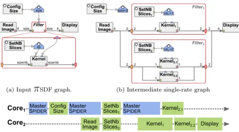
π

SDF graph on a multicore architecture. The input

π

SDF graph considered in this example is depicted in Figure 12a, and Figure 12b illustrates an in-termediate graph resulting from graph tranformations applied at runtime by the Spider runtime, prior to mapping and scheduling operation. The Gantt diagram corresponding to an iteration of this graph on 2 cores is presented in Figure 12c. The master process of the Spider runtime is called at the

size Config

Size

Filter Read

Image 4 size size 4 Display

nb SetNB Slices

size/nb Kernelsize/nb

(a) Input

π

SDF graph.

size=2 Config Size Read Image 4 2 2 4 Display nb1=1 SetNB Slices1 2 Kernel12 2 2 Filter1 2 2 nb2=2 SetNB Slices2 1 Kernel2.11 2 2 Filter2 Kernel2.2 1 1

(b) Intermediate single-rate graph Core1

Core2

Master

SPIDER ConfigSize SMasterPIDER Read Image SlicesSetNb2

SetNb Slices1 Master SPIDER Kernel1 Kernel2.2 Kernel2.1 Display (c) Gantt diagram of one iteration of the

π

SDF graph with Spider. Fig. 12 Deployment process of the Spider runtime.

beginning of the execution, in order to map and schedule the ConfigSize con-figuration actor that is, at this point, the only executable actor according to

π

SDF execution rules. When executed, the ConfigSize actor sets a new value for parameter size triggering a reconfiguration, and a second call to the master process. Using the new value of the size parameter, the master process computes the repetition vector of the top-level graph and applies a single-rate graph transformation in order to expose its data-parallelism. With size = 2, the single-rate transformation duplicates the Filter actor to make the data-parallelism of its two firings explicit. At this step, memory can be allocated for all Fifos of the top-level graph, and the ReadImage actor can be scheduled. Concurrently to the execution of the ReadImage actor, the master process continues its execution to manage the execution of the two instances of the Filter hierarchical actor. The master process manages separately the two subgraphs of the Filter actors, and schedules a firing of the SetNBSlices configuration actor for each of them. During the third and final call to the master process, a new configuration of each of the two subgraphs is taken into account to compute their respective repetition vectors, to perform the single-rate graph transformation on them, to allocate all Fifos in memory, and to schedule all remaining actor firings. The single-rate graph of Figure 12b is the executed graph for parameter values size = 2, nb1= 1, and nb2= 2.

Compared to implementation strategies with no global management of applications, using a runtime manager to control the execution of a recon-figurable graph has an overhead on application performance. Indeed, such runtime manager requires processor time to compute repetition vectors, to perform graph transformations, and to map and schedule actor firings.

Nev-ertheless, as presented in [29, 28], even with large reconfigurable graphs with several hundreds of actors, this overhead is largely compensated by the ef-ficiency of the scheduling decisions, and generally outperforms dynamic de-ployment strategies with no global manager.

3.3 Compilation Flow for SPDF Graphs

A compilation framework for deploying reconfigurable applications specified with the SPDF MoC onto heterogeneous MPSoCs is presented in [16]. This development flow for SPDF graphs differs from the flow based on the runtime manager presented in the previous section in that it shifts most of the de-ployment decisions to the compilation framework. In particular, in the SPDF compilation flow, actors are manually mapped on the cores by the appli-cation designer, and actor firings are quasi-statically scheduled based on a compile-time analysis of the graph and the behavior of actors. An overview of the different stages of the SPDF compilation flow, adopting the elements presented in Chapter [39], is illustrated in Figure 13.

Front-end Developer Reduced SPDF Graph Actor Code Heterogeneous MPSoC Application Specification P

a

D

a

F (C++) CLang Reduced_PaDaF (LLVM IR) SPDF Graph (PaDaF IR) Actor + annota-tions (LLVM IR) Execution Analysis Link _PaFull_DaF (PaDaF IR) Check buffer Map/Schedule Codegen (ASM) Back-end

Fig. 13 Overview of the compilation flow for SPDF graphs [16]

In the SPDF compilation flow, the specifications of both the SPDF graph and the internal behavior of actors are based on a hierarchy of specialized C++ classes called Parametric Dataflow Format (padaf). Figure 14 illus-trates the syntax used to specify part of an LTE application with padaf [16]. The SPDF graph presented in Figure 14a contains a parameterizable number N b of FFT actors, each processing 1024 samples received from an antenna. Results of the FFT actors are then transmitted to a MIMO actor, which sets a new value for parameter p at each firing, and produces a reconfigurable number of data tokens towards the Sink actor. As shown in the C++ de-scription of the LTE graph in Figure 14b, padaf allows the dede-scription of SPDF graphs using for-loop constructs. Hence, the padaf syntax specifies SPDF graphs in a reduced format where a statically parameterizable num-ber of actors and Fifos may be instantiated and connected together. This syntax is similar to the SigmaC programming language used for the

specifi-cation of decidable CSDF graphs [25]. The padaf code corresponding to the MIMO actor is presented in Figure 14c. As can be seen in this example, actor specification is based on a hierarchy of C++ classes used to specify actors (Actor class), their data ports (PortIn/PortOut classes), and their parame-ters (ParamOut class). As in graph descriptions, control code can be used to specify a statically parameterizable number of data ports when specifying an SPDF actor with padaf. The internal computations performed by an actor at each firing are specified in its unique compute() function.

1024 FFT1 600 1024 FFT2 600 1024 FFTNb 600 set p[1] MIMO57p Sink 4200 4200 4200 57 (a) SPDF graph. Fft fft[N B _ A N T]; M i m o m i m o; S i n k s i n k; for(i=0; i<N B _ A N T; i++) { fft[i].out <= m i m o.in[i]; } s i n k.in <= m i m o.out

(b) padaf graph description.

c l a s s M i m o : p u b l i c A c t o r {

std::vector<PortIn<int>* > Iin;

PortOut<int> I o u t; P a r a m O u t p; int n b A n t M i m o(int nb) : p(1) , out(p* 5 7 ) { n b A n t = nb; for(int i=0; i<nb; i++) {

Iin[i] = new PortIn<int> ( 4 2 0 0 ) ; }

}

v o i d c o m p u t e() ;

}

(c) padaf Mimo actor code.

Fig. 14 Partial LTE application specification with padaf (From [16])

The steps composing the compilation flow presented in Figure 13 are sorted into two groups, the front-end and the back-end, presented hereafter. • Front-end : The first steps of the SPDF compilation flow, called the

front-end, are architecture-independent operations responsible for expos-ing coarse and fine grain properties of the application.

– Clang: The first step of the front-end is to compile the graph and the actor padaf specifications of an application into an LLVM Intermediate Representation (IR) using the Clang compiler [36].

– Execution: In a second step, the produced LLVM IR corresponding to the reduced graph description is executed in order to build the complete SPDF graph, where a parameterizable number of actors are instanti-ated.

– Analysis: In the third step of the front-end, executed in parallel with the second, the LLVM IR corresponding to the internal behavior of actors

is analyzed in order to detect and annotate the instructions responsible for pushing and popping data into the Fifos connected to each actor. – Link : In the last step of the front-end, a full padaf IR of the application

is obtained by linking the complete SPDF graph with annotated actor code, as detailed in [16].

• Back-end : The latter steps of the compilation flow, called the back-end, are responsible for deploying the application on a specified heterogeneous architecture.

– Map/Schedule: Although mapping of the actors is currently manually specified by the application developer, the back-end is still responsible for producing a quasi-static schedule of actor firings for each core. – Check buffer : An analysis of the proposed mapping and scheduling is

also used to check that the memory capacity of the targeted platforms are not exceeded.

– Codegen (Assembly (ASM))Finally, the annotated internal data access patterns of actors exposed in the padaf IR are used in the code genera-tion step in order to generate calls to on-chip communicagenera-tion primitives, and to produce efficiently pipelined ASM code.

The efficiency of this SPDF compilation flow is demonstrated in [16] for the deployment of several Software Defined Radio (SDR) applications on a domain-specific MPSoCs. The performance of the synthesized software for evaluated SDR applications is shown to be equivalent to handwritten code.

3.4 Software Reconfiguration for Dynamic Dataflow

Graphs

Applications specified with dynamic dataflow MoCs do not, in general, ex-hibit a safe reconfigurable behavior as defined in Section 2.1. Hence, software implementation techniques presented in previous sections that exploit the compile-time and runtime predictability of reconfigurable behavior can not, in general, be applied to dynamic dataflow graphs. This section presents how a design flow integrating reconfigurable software components can be used to improve the implementation of dynamic dataflow graphs. Here, a software component designates an application independent piece of software support-ing the execution of a dynamic dataflow graph by managsupport-ing and monitorsupport-ing its deployment onto a target architecture. Reconfigurability of these software components comes from their capability to change their deployment strategies at runtime in order to impact a performance indicator (e.g. latency, energy consumption, ...), in a controlled and predictable way.

Figure 15 presents an overview of an energy-aware design flow, proposed in [55], for video decoding applications specified with dynamic dataflow graphs. The design flow is composed of three main parts:

1. a modular specification of the application based on a dynamic dataflow MoC [64],

2. reconfigurable software components controlling the energy of the deployed application

3. a hardware platform embedding energy and performance sensors

RVC-CAL Standard Video Decoding Building Blocks Video Decoder Networks Compose JADE

(Just-in-time Adaptive Decoder Engine)

Reconfiguration Engine Hardware Platform Just-In-Time Compilation Energy Manager Monitor Trigger Perf. Counter Battery Level Feed Select Input Bitstream Decoded Video

Fig. 15 Overview of an energy-aware design flow for dynamic dataflow graphs [55].

Rvc-cal [10] is a language standardized by the Motion Picture Expert Group (MPEG) committee to specify video decoders. In Rvc-cal, a set of widely used video decoding basic building blocks, like discrete cosine trans-forms, variable length coding algorithms, or deblocking filters, can be com-posed into a network in order to specify a complete video decoder. Network specified with Rvc-cal implements the Dataflow Process Network (DPN) semantics [38], which is a non-deterministic model close to the CFDF MoC. Rvc-cal descriptions of several video decoders with diverse computational complexity are used as inputs of the design flow presented in Figure 15.

The Just-in-time Adaptive Decoder Engine (Jade), which constitutes the second stage of the design flow presented in Figure 15, is a software compo-nent built with LLVM [24]. The main purpose of Jade is to manage on-the-fly the execution of platform-independent Rvc-cal networks onto various hard-ware platforms. To do so, Jade translates a selected network of Rvc-cal actors into the LLVM IR, and feeds it to the just-in-time LLVM compiler and interpreter for the targeted platform.

The energy manager that was integrated within Jade in [55] is the key reconfigurable software component of the design flow presented in Figure 15. The first objective of the energy manager is to monitor the execution of the application on the targeted platform in order to build an energy model of its energy consumption [55]. Monitoring of the application is achieved by automatically inserting calls to instrumentation functions reading perfor-mance monitoring counters of the targeted platform. Using the energy model

built from monitoring information, the energy manager is able to estimate precisely the energy consumption of the different video decoders at its dis-position. The second responsibility of the energy manager is to control the energy consumption of the system by triggering reconfigurations of the cur-rently executed network. A typical scenario for reconfiguration occurs when the energy manager estimates that the remaining battery charge is insuffi-cient to finish decoding a video stream of known length. In such a scenario, the energy manager may trigger a reconfiguration to a different network with lower computational complexity and lower quality, but which will reduce en-ergy consumption. Practical evaluation of this enen-ergy-aware design flow [55] shows the efficiency of this approach on the latest HEVC video standard.

Further work on the use of software reconfiguration techniques for imple-menting dynamic dataflow MoCs is presented in [68]. In this work, a low-cost monitoring of the execution all actors of a DPN is used to obtain statistics on their execution time. Using this monitoring information, a runtime manager may trigger a reconfiguration of the mapping of the different actors on the different Processing Element (PE) of the targeted architecture.

4 Dataflow-Based Techniques for Hardware

Reconfigurable Computing Platforms

Flexibility and adaptivity of a signal processing system at the hardware level may be achieved by means of reconfigurable computing. In recent years, re-configurable computing has become a popular hardware design paradigm for accelerating a wide variety of applications. Hardware reconfiguration is com-monly used as a way to enable kernel execution over specialized and optimized circuits, retaining much of the flexibility of a software solution.

Figure 16 depicts a very general overview of the classical computing spectrum, whose extremes are represented by Central Processing Units (CPUs) -generic and extremely flexible - and Application Specific Integrated Circuits (ASICs) - dedicated, non programmable, circuits customized and highly op-timized for a given functionality. CPUs are capable of executing any type of code their compilers can translate into machine code, with average perfor-mance and very limited optimization capabilities. The flexibility of CPUs comes at the expense of - medium to highly - complex hardware micro-architectures requiring a significant amount of silicon area for their imple-mentation to be able to serve a complete instruction set. In ASIC designs, resources are minimized since the architecture is forged accordingly to the native execution flow of the implemented application, while operating fre-quency, throughput and energy consumption may be optimized according to the given constraints. A counterpart of this highly optimized design is that ASICs are not flexible at all, as their hardwired datapath can execute no other function than the one they are meant for. Reconfigurable computing

infrastructures lays in between, representing an appealing option since they are capable of guaranteeing a trade-off among the aforementioned extremes. In practice, reconfigurable hardware allows customizing the execution infras-tructure by allowing runtime (re-)programmability of datapaths to imple-ment application-specific datapaths, thus providing flexibility. Switching and programmability capabilities determine the type of implementable reconfig-uration that, as discussed hereafter, can take place at different granularities.

DSP ASIC GPU CPU General Purpose Flexibility Performance Fine

Grained Grained Coarse

Reconfigurable

Fig. 16 Overview of the classical computing spectrum: performance versus flexibility.

Studies on the subject of reconfigurable hardware dates back to nineties and have been surveyed in several different works along time [15, 27, 34, 62, 63, 65]. Reconfigurable hardware guarantees different degrees of flexibility, being (re-)programmable over a given set of functionalities, but still offering specialization advantages. Nevertheless, as in any specialized design, pro-grammability design does not come for free: it requires the programmers to have a deep knowledge and understanding of the architectural details. This drawback traditionally limited the wide usage of reconfigurable computing systems. Field Programmable Gate Array (FPGA) platforms, for example, were typically considered merely as development boards for prototyping ac-tivities, rather than an actual target.

The main purpose of this section is to understand how dataflow-based specifications and design flows can be used to facilitate the design of recon-figurable computing infrastructures. Before that a bit of terminology has to be introduced. Different types of classification of reconfigurable computing systems are available. We will refer hereafter mainly to coarse grained (CG) and fine grained (FG) reconfigurable platforms. These two types of architec-tures differ for the size of the hardware blocks that are reconfigured. • Coarse Grained (CG) reconfigurable computing systems involve a fixed set

of - often programmable - Processing Elements (PEs) connected by means of dedicated routing blocks [15]. The basic idea behind these systems is to maximize resource re-use among different target applications. PEs are managed in a time multiplexed manner to serve different functionalities at different execution instants. The number of interchangeable scenarios is typically fixed and at runtime the system can switch from one execution to another.

• Fine Grained (FG) reconfigurable computing systems can execute a theo-retically infinite number of different functions, since programmability takes