HAL Id: hal-03190672
https://hal.archives-ouvertes.fr/hal-03190672
Submitted on 6 Apr 2021
HAL is a multi-disciplinary open access
archive for the deposit and dissemination of
sci-entific research documents, whether they are
pub-lished or not. The documents may come from
teaching and research institutions in France or
abroad, or from public or private research centers.
L’archive ouverte pluridisciplinaire HAL, est
destinée au dépôt et à la diffusion de documents
scientifiques de niveau recherche, publiés ou non,
émanant des établissements d’enseignement et de
recherche français ou étrangers, des laboratoires
publics ou privés.
SUPPLY CHAIN ROUTING SCHEDULING
SUB-MODEL DESIGN: CASE OF EXPORT BULK
PORTS
S Mallah, A Aloullal, O Kamach, M. Masmoudi, N Najid, K. Kouiss, L
Deshayes
To cite this version:
S Mallah, A Aloullal, O Kamach, M. Masmoudi, N Najid, et al.. SUPPLY CHAIN ROUTING
SCHEDULING SUB-MODEL DESIGN: CASE OF EXPORT BULK PORTS. 13ème CONFERENCE
INTERNATIONALE DE MODELISATION, OPTIMISATION ET SIMULATION (MOSIM2020),
12-14 Nov 2020, AGADIR, Maroc, Nov 2020, AGADIR (virtual), Morocco. �hal-03190672�
SUPPLY CHAIN ROUTING SCHEDULING SUB-MODEL DESIGN: CASE
OF EXPORT BULK PORTS
S. Mallah*, ** & A. Aloullal*
*ILO – University Mohammed 6 Polytechnic (UM6P), Bengueir, Morocco
**LTI – National School of Applied Sciences –
Ab-delmalek Essaadi University (AEU), Tangier, Morocco [email protected]/[email protected],
O. Kamach*, **, M. Masmoudi***, N. Najid****, K. Kouiss*,*****, L. Deshayes*
***University Jean-Monnet, France **** Mechanical and Productive Engineering
Depart-ment, University of Nantes, France
*****SIL – Blaise-Pascal, university of Clermont Fer-rand, Aubière, France
[email protected], [email protected], [email protected],
[email protected], [email protected]
ABSTRACT: The integration of planning and scheduling decisions of loading, stacking/scraping, routing and
produc-tion making up an integrated optimizaproduc-tion plan without contradictory goals is vital for an efficient use of the four afore-mentioned bulk port operations. While the research community debates on how to integrate these different decisions in one model and thus to get the four problems optimized simultaneously, in this paper, conversely though, another integra-tion approach is presented. However, the main contribuintegra-tion is the formulaintegra-tion of the problem as a mixed integer linear program, in such a way to comply with the other operations decisions and to reflect the real aspects of the industrial settings. Due to the integration approach used, the routing model has had many constraints relaxed, compared to other routing models, while still considering all the specifications of the dynamic export bulk port environment.
KEYWORDS: Port sub-problems, scheduling sub-models integration, routing sub-model, conveyors paths.
1 INTRODUCTION
In order for an export bulk terminal to deliver the right product, with good quality, to the right customer, in the right place and at the right time, an optimization of its lo-gistics process is essential to set up. The case study in this work deals with an optimization which aims to return, in a reasonable planning time, an integrated operations plan maximizing the loading capacities over a planning hori-zon of tactical level. Where each of the four sub-problems (loading, stock, routing and production) making up the overall port optimization problem must maximize the loading capacities taking into account the other logistics operations which may have contradictory goals.
An alternative to planning and scheduling the port opera-tions in an integrated approach, considering the four sub-problems in one mathematical model is to integrate the planning sub-problems as separated sub-systems interact-ing with each other in a smart fashion. The rational behind this alternative is because the integrated approach may lead to an optimization result which does not include all the specifications reflecting reality or that does not con-verge. Similarly, the option of treating each of these sub-problems separately has raised two very important ques-tions:
• How to manage the interactions between the four sub-models so that the planning system converges in a reasonable response time and avoids quasi infinite interaction loops between the three sub-models?
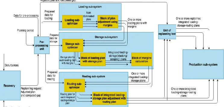
• What are the decision variables, the objective-func-tions and the constraints of each sub-model, pro-vided that consistency and avoidance of redundancy between the four sub-models are maintained? The sheer size of work necessary to answer the aforemen-tioned questions is detailed in [1] which specifies the in-tegration of the planning sub-systems, but also the inte-gration of the planning tool with the control system. For the sake of simplicity, Figure 1 presents the spirit of this work. It illustrates the coupling strategy between the four sub-systems of the planning tool while neglecting the in-teraction with the control system. However, it clearly shows the interaction scenarios between the planning and scheduling sub-systems. In fact:
The loading sub-system returns a set of loading plans
re-specting the commercial plans of ships and trucks. It will also adjust each loading plan in such a way as to provide more flexibility in terms of margins without modifying the final result. The latter aims at maximizing the total volume loaded and minimizing the sum of late penalties.
The stock sub-system returns for each loading plan with
margins a stacking and scraping plan respecting the load-ing time windows by minimizload-ing, for each demand, the gap between stock operations date and loading date with margins included. Then, by integrating the two loading and stock plans, it will adjust the loading periods if nec-essary. Finally, it will define for each plan resulting from the integration of stock and loading the remaining margins of the margins of the loading plan or new margins from the new loading-stock plan.
MOSIM’20 – November 12-14, 2020 - Agadir - Morocco
The routing sub-system is composed of:
a. A routing sub-optimizer whose development is the
objective of this document. Its mission is to return for each request of the integrated plan (loading-stock) a routing plan respecting the stacking, scraping and loading time windows by minimizing, for each demand, the gap from loading and stock dates with margins included, and by selecting paths with early and short transportation service.
b. The plan adjustment block integrated with the
routing, by integrating the loading, stock and routing plans, will adjust the loading and stock periods if necessary. Thus, we obtain the integrated loading, stock and routing plans.
The production sub-system returns a production plan for
each integrated loading-stock-routing plan and adjusts the periods of operations if necessary.
The aspect of disturbances is dealt with by the recovery tool, which manages to generate an adjusted plan and to compute the gap between the plan before and after adjust-ment. If the gap is not significant, the adjusted plan is ex-ecuted by the control system. Otherwise, the recovery re-quests the planning tool to reschedule. This is where the rescheduling test unit comes in to compare the resched-uled plan with the adjusted plan and give the best out of the comparison.
The development of each subsystem of the planning and scheduling system is the step that follows the coupling strategy. The development of the routing sub-optimizer, in particular, is the main objective of the remainder of this paper. Which is structured as follows: related works con-cerning the planning and scheduling of bulk port problems
are provided in section 2. Section 3 will describe the prob-lem at hand. Section 4 will give a mathematical formula-tion of the routing problem. Finally, a conclusion and per-spectives are given in section 5.
2 LITERATURE REVIEW
The belt-conveyors routing scheduling problem in bulk port has just been studied recently [2]. In fact, enormous efforts have been rather made toward optimizing transpor-tation problems in container port terminals, which implies without having the belt-conveyors routes as a means of transportation [3, 4, 5, 6]. The authors of [3] tackled trans-portation systems for container port logistics by focusing mainly on task assignments problems or routing problems for automated guided vehicles, while the authors of [4] solved multi-trailer transportation routing problem and in [5], the authors solved the routing problem for a fleet of trucks with different capacities. The authors of [6], on the other hand, worked on the container allocation and the straddle-carrier routing problem. Apart from container ports, the transportation optimization was studied in a general context in [7] which studies the vehicle routing and truck driver scheduling problem where routes and schedules must comply with hours of service regulations for truck drivers. Therefore, as bulk ports started to re-ceive a growing interest conveyors-belt based transporta-tion optimizatransporta-tion is strongly demanded. In this paper, we are focused on the belt-conveyors routing scheduling problem, in bulk ports, in such a way to comply with the other operations planning and scheduling decisions, namely: stock management and reclaiming problem and berth allocation problem.
From the earliest work, we can find the work of [8] where the authors dealt with the belt-conveyor transportation routing problem along with the storage allocation problem
where requests are given in real time. They provided a for-mulation of the problem using a mixed integer program-ing approach and proposed a Lagrangian decomposition to solve it and compared it with the hierarchical planning method.
In the same perspective, the authors of [2] dealt with the conveyor-belt transportation routing optimization along with stockyard optimization in an integrated fashion, while calling the integrated problem as the Product Flow Planning and Scheduling Problem. But they also consid-ered more constraining aspects, compared to [8], such as route allocation constraints, product scheduling con-straints and equipment capacity concon-straints.
Similar to the ambitious work toward integrating the set of bulk port operations planning and scheduling decisions, we have already proposed in [1] an integration approach that consider optimizing loading, stacking/scraping, rout-ing and production problems. In fact, instead of consider-ingone mathematical model that would lead to uncontrol-lable complexity, or to an optimization result that miss real industrial use cases, and that wouldn’t converge, we actually proposed to integrate the planning and scheduling sub-problems as separated sub-systems interacting with each other without falling in quasi-infinite interaction loops. And to the best of our knowledge, there is no opti-mization work in the literature that takes the interactions between subsystems into account before moving to the optimization of each subsystem, although these interac-tions cannot be neglected in a real case, otherwise, the re-turned solution of each subsystem will be biased. Besides, since the integration approach proposed in [1] managed to maintain consistency and avoidance of redundancy be-tween the sub-models in terms of decisions, thus in terms of decision variables, constraints and objective functions. Then, as a result, the routing sub-model, has its constraints relaxed given that all the dynamic aspects of a real indus-trial setting are considered including the real conveyors paths matrix structure. In this paper, we are going to pro-pose the model of the routing scheduling sub-problem.
3 PROBLEM DESCRIPTION
The problem investigated in this paper is motivated by a real case dealing with the planning and scheduling of an export bulk port. In order to fulfill its mission which is to supply the end customer (trucks / ships) with the requested product, the terminal possesses several types of equip-ment: stacker for stocking products, scrapers to scrape or destock the products, belt conveyors to transport products from a source to a destination, and gantry cranes to load ships. The trucks are loaded directly by pouring the prod-uct, contained within the belt conveyor, into the truck. The products moved through the port concern fertilizers and phosphates whose qualities differ in their chemical and physical characteristics such as granularity. Thus, for fer-tilizers and phosphates, there is a whole host of ranges or families of products and each of these ranges includes a whole set of qualities amounting to about 40 qualities.
The port platform is made up of four subsystems which are: the fertilizer and phosphate production lines, the stor-age sheds where the two operations of stacking and scrap-ing are carried out, the set of conveyor routes for the transport and finally the loading stations, be it the berths for loading ships or the loading stations for trucks. The production subsystem consists of several sets of pro-duction lines. In our case, these are four sets of propro-duction lines. Each set of production lines is connected to a unique set of the storage subsystem. Given that each set of the storage subsystem is composed of several hangars where different qualities of the products are stored.
The storage subsystem automatically includes four stor-age sets: A, B, C for the storstor-age of fertilizers, and D for the storage of phosphates. All storage subsystems are sup-plied with products from their own factories. The stock subsystem B, in particular, can also receive products from the storage set: A.
The loading subsystem includes a trucks loading stations set and a vessels loading set. The trucks loading set con-sists of loading stations where each station manages to load a truck with product from the storage sets A and B only. While the vessels loading set is made up of several berths each housing a set of gantry cranes for loading ves-sels with products from all the storage sets: A, B, C, and D.
The routes subsystem is a combination of routes defining several path options through which products can be routed between the different subsystems. Many routes share common conveyors, so if products of different demands are to be transported at overlapping time intervals, they must be assigned to routes that do not overlap. Each route has a predefined capacity which must be respected. Figure 2 shows a general schematic about the four subsystems of: production, storage, loading and routes without represent-ing the extreme degree of complexity of each of them. For instance, the conveyor routes combination whose each line illustrated in the figure refers to a whole combined set of paths.
In this paper, as already mentioned, the interest is focused on the routing sub-problem in particular. In addition, the port of the case study does not raise any need for optimi-zation involving transport from the production lines since each storage shed has a production plant which supplies it with product. The need for optimization lies in the net-work between the storage and loading subsystems. In fact, the sets of the storage subsystem are not of the same kind, thus constituting six sources instead of the four already mentioned: A, B, C, D. To detail this further, each set of {A, C, D} is a homogeneous set. Which means that all the hangars of the same set have the same characteristics. Conversely though, the set B consists of hangars which do not have the same characteristics, thus generating three subsets of the set B.
MOSIM’20 – November 12-14, 2020 - Agadir - Morocco
More precisely, each of {A, C, D} is a set of hangars: • Where each hangar has only one entrance or input,
making it one destination at a time.
• Where each hangar has only one exit or output, mak-ing it one source at a time.
• The maximum output capacity is the same for all hangars in the same set: capacity C1 for sources in set A, and capacity C2 for sources in sets C and D. Given that C2 is greater than C1.
While set B is special in all aspects. It consists of hangars: • Where each hangar has only one entrance, making it
one destination at a time.
• The maximum entry capacity is the same for all hang-ars, which is C3.
• Where a subset of hangars B is at a single outlet mak-ing each of them a smak-ingle source at a time with a max-imum capacity C2.
• Whereas another subset of hangars B has two exits, making each of them two sources which, in turn, are not, are not homogeneous. Because the two sources are at a maximum capacity C1 and C2 respectively. The loading subsystem is made up of destinations with different maximum capacities: C4 for trucks loading sta-tions and C1 and C2 for berths gantry cranes.
The routing sub-model is intended to transport the prod-ucts between the sets of the storage subsystem and be-tween the storage and loading subsystems according to the loading-stock plan. This refers to transporting the prod-ucts from six sets of sources: {A, B (including its three subsets), C, D} whose capacity belongs to the set of ca-pacities {C1, C2} to the set of destinations {B, trucks loading set, vessels loading set} whose capacity belongs to the set of capacities {C1, C2, C3, C4} Given that: C3 <C4 <C1 <C2. Thus, making a combinatorial game of very complicated routing conveyors. To fully understand the matrix of conveyor routes, we have classified the routes into ten types. Each type composes a set of routes with the same source set, the same destination set and whose maximum capacity is equal to the minimum capac-ity of the source and the destination. Hence, for each lo-gistics operation, the path that ensures a minimal tardiness and waiting time that can be selected from a subset of routes 𝑹𝒌 instead of all of the routes set 𝑹. This will con-tribute in reducing the complexity while generating the routing plan. All of these ten routes classes include:
• 𝑹𝒙: the routes formed from the exits of the hangars of set A, to the entrances of set B with a capacity C3. • Rs: the routes formed from the exits of the hangars of
set A, to trucks stations with a C4 capacity.
• Ry: the routes formed from the exits of the hangars of set A, to the berths gantry cranes with C1 capacity. • Rt: the routes formed from the exits of the hangars of
set B (the three sub-sets of B included), to trucks sta-tions with C4 capacity.
• Rzsmall: the routes formed from the exits of the hangars of set B (the three subsets of B included), to the berths gantry cranes with capacity C1. The term "small" re-fers to the fact that loading of ships is possible on two capacities: C1 and C2. Except that C1 is smaller than C2.
• Rzbig: the routes formed from the exits of the hangars from set B (only two subsets of B included: hangars with only one exit with capacity C2, and hangars with 2 exits and precisely from exits whose capacity is C2), up to ship berths gantry cranes with capacity C2. The term "big" refers to the fact that loading of ships is possible on two capacities: C1 and C2. And C2 is the maximum capacity.
• Rvsmall: the routes formed from the exits of the hangars of set C to the berths gantry cranes of ships with a ca-pacity of C1.
• Rvbig: the routes formed from the exits of the hangars from set C to the berths gantry cranes with C2 capac-ity.
• Rwsmall: the routes formed from the exits of the hang-ars of set D to the berths gantry cranes with C1 capac-ity.
• Rwbig: the routes formed from the exits of the hangars of set D to the berths gantry cranes with C2 capacity. The combination of these paths has of course given pos-sible overlaps within each type of routes and between dif-ferent types.
All of the points described so far are illustrated in the schematic of Figure 3.
The possible overlaps between routes belonging to the same routes type and between routes of different types are illustrated in table 1.
The optimization problem that motivated this study con-cerns a routing problem that focuses on scheduling deci-sions without having to deal with planning decideci-sions. Be-cause the integration approach adopted in [1] and ex-plained in the previous sections, resulted in having plan-ning and scheduling decisions for both the loading and stock problems. In fact, the integrated loading-stock plan sets the transportation time window (with stacking and scraping/loading margins included) in which each de-mand needs to be transported and defines the source and the destination of its qualities (products). Which led to re-duce the routing decisions down to scheduling decisions that choose from the subset of routes defined for each quality of a demand, the one that guarantee a minimal gap with regards to loading and stock dates, and an early
MOSIM’20 – November 12-14, 2020 - Agadir - Morocco
transport with minimal transfer time, in case the gap is null. These two objectives aim to guarantee that the ships and trucks will be loaded with the required products on schedule provided all the constraints are respected, such as the prohibition of routes overlaps. In the remainder of this article, this problem will be called the Product Rout-ing SchedulRout-ing Problem, or PRSP.
Table 1 - Overlaps between routes
Routes type Itinerary Overlap with
Routes S (𝑅𝑆) A – Trucks loa-ding stations
𝑅𝑆, 𝑅𝑇, 𝑅𝑋,
𝑅𝑌, 𝑅𝑍𝑠𝑚𝑎𝑙𝑙
and 𝑅𝑍𝑏𝑖𝑔
Routes T (𝑅𝑇) B – Trucks loa-ding stations
𝑅𝑇, 𝑅𝑆, 𝑅𝑍𝑠𝑚𝑎𝑙𝑙, 𝑅𝑍𝑏𝑖𝑔 and 𝑅𝑌 Routes X (𝑅𝑋) A – B 𝑅𝑋, 𝑅𝑌, 𝑅𝑆 Routes Y (𝑅𝑌) A – Loading berths with ca-pacity C1 𝑅𝑌, 𝑅𝑆, 𝑅𝑋, 𝑅𝑇, 𝑅𝑍𝑠𝑚𝑎𝑙𝑙, 𝑅𝑍𝑏𝑖𝑔, 𝑅𝑉𝑠𝑚𝑎𝑙𝑙, 𝑅𝑊𝑠𝑚𝑎𝑙𝑙 Routes Z Routes 𝑍𝑠𝑚𝑎𝑙𝑙 (𝑅𝑍𝑠𝑚𝑎𝑙𝑙) B – Loading berths with ca-pacity C1 𝑅𝑍𝑠𝑚𝑎𝑙𝑙, 𝑅𝑍𝑏𝑖𝑔, 𝑅𝑆, 𝑅𝑇, 𝑅𝑌, 𝑅𝑉𝑠𝑚𝑎𝑙𝑙, 𝑅𝑊𝑠𝑚𝑎𝑙𝑙 Routes 𝑍𝑏𝑖𝑔 (𝑅𝑍𝑏𝑖𝑔) B – Loading berths with ca-pacity C2 𝑅𝑍𝑏𝑖𝑔, 𝑅𝑍𝑠𝑚𝑎𝑙𝑙, 𝑅𝑆, 𝑅𝑇, 𝑅𝑌, 𝑅𝑉𝑏𝑖𝑔 Routes V Routes 𝑉𝑠𝑚𝑎𝑙𝑙 (𝑅𝑉𝑠𝑚𝑎𝑙𝑙) C – Loading berths with ca-pacity C1 𝑅𝑉𝑠𝑚𝑎𝑙𝑙, 𝑅𝑉𝑏𝑖𝑔, 𝑅𝑌, 𝑅𝑍𝑠𝑚𝑎𝑙𝑙, 𝑅𝑊𝑠𝑚𝑎𝑙𝑙 Routes 𝑉𝑏𝑖𝑔 (𝑅𝑉𝑏𝑖𝑔) C – Loading berths with ca-pacity C2 𝑅𝑉𝑏𝑖𝑔, 𝑅𝑉𝑠𝑚𝑎𝑙𝑙, 𝑅𝑍𝑏𝑖𝑔, 𝑅𝑊𝑏𝑖𝑔 Routes W Routes 𝑊𝑠𝑚𝑎𝑙𝑙 (𝑅𝑊𝑠𝑚𝑎𝑙𝑙) D – Loading berths with ca-pacity C1 𝑅𝑊𝑠𝑚𝑎𝑙𝑙, 𝑅𝑌, 𝑅𝑍𝑠𝑚𝑎𝑙𝑙, 𝑅𝑉𝑠𝑚𝑎𝑙𝑙 Routes 𝑊𝑏𝑖𝑔 (𝑅𝑊𝑏𝑖𝑔) D – Loading berths with ca-pacity C2
𝑅𝑊𝑏𝑖𝑔, 𝑅𝑉𝑏𝑖𝑔
4 PRSP FORMULATION
The mathematical model receives the planning of demands from the loading and stocking sub-systems, where each demand is characterized by a list of qualities (products) that should be transported to a destination. The time window of each demand is known, as well as the source and destination of each quality that make us define the subset of routes 𝑹𝒅𝒒 (from 𝑹𝒌) rather than the whole set 𝑹. The routing sub-optimizer aims to find for all demands, the routes that minimize the sum of tardiness penalties and waiting costs. Given that:
• The tardiness is the positive value of the real final date (of the transportation service) minus the expected final date (of the transportation service) [9].
• The waiting time is the real starting date (of the transportation service) minus the expected starting date (of the transportation service) plus the transfer time.
In fact, the transport time of one quality in a route is equal to its transfer time that presents the amount of time needed for a flow to arrive from the source to the destination of the route plus the period of stacking or scraping/loading needed to satisfy the total of the quantity requested. The transfer time is related to the decision variable of the chosen route, while the stacking or scraping/loading period is a parameter equal to the quantity requested divided by the stacking or scraping/loading rate returned from the stock-loading sub-systems.
All demands are planned for a given time horizon H, divided into periods µ. Routes are classified into classes presented in the section before.
The main challenge of the following model is the scheduling of routes to fulfill the demand while minimizing tardiness penalties and waiting cost for each demand.
Hypotheses:
• The transport of a demand must be continuous, i.e. no suspension is authorized between the transport of the qualities requested, except the time needed between successive ones.
Notation:
𝐻 The time horizon ⟦0,𝐻𝑚𝑎𝑥− 1⟧ ; divided into µ periods
𝐻𝑚𝑎𝑥 the total number of µ periods in the time horizon
𝑅 The set of routes 𝐸 The set of equipment
𝑅𝑒 The set of routes that share the same equip-ment e; 𝑒 ∈ 𝐸
𝑅𝑘 The set of routes, Rk∈ {Rx, Rs, Ry, Rt,
Rzsmall, Rzbig, Rvsmall, Rvbig, Rwsmall, Rwbig}
𝐷 The set of demands; = {1, …, 𝑛𝐷} 𝑛𝐷 The number of total demands
𝑄𝑑 The set of qualities (products) of the demand
𝑛𝑄𝑑 The total number of qualities of demand d 𝑛𝑄𝑡𝑜𝑡𝑎𝑙 = ∑ 𝑛𝑄
𝑑 𝑑∈𝐷
𝑃𝑟𝑒𝐿𝑖𝑠𝑡 A set of demand pairs that present all combi-nations of demand precedence; (𝑑, 𝑑′) ∈ 𝑃𝑟𝑒𝐿𝑖𝑠𝑡 ∶ (the final date of transporting the demand d should be before the start date of transporting the demand d’)
𝑖𝑛𝑡𝑒𝑟𝐷𝑑𝑑′ The time needed between transporting the demand d and d’
𝑠𝑡𝑑 𝑠 The start time of the transportation service of demand d
𝑠𝑡𝑑 𝑓 The end time of the transportation service of demand d
𝐻𝑑 Transportation horizon of the demand d; = ⟦𝑠𝑡𝑑 𝑠,𝐻𝑚𝑎𝑥− 1⟧ ; divided into µ periods 𝑅𝑑𝑞 A subset of 𝑅𝑘 contains all the routes that
link the source from where the quality q of the demand d is transported, with its destina-tion
ℎ𝑑𝑞 The stacking or scraping/loading period to satisfy the quality q of the demand d 𝑖𝑛𝑡𝑒𝑟𝑄 The time needed between the transport of two successive qualities of the same demand; it is fixed for all demands
𝑡𝑡𝑟 The time required for the route r to transfer a quality from its source to its destination (transfer time of the route r)
𝐶𝑟 The capacity of each route r
𝑒𝑞𝑒𝑟 Equals to 1 if the equipment e belongs to the route r, and equals to 0 otherwise.
𝑃𝑒𝑛𝑎𝑙𝑡𝑦𝑑 Tardiness penalty for the demand d
𝑊𝐶𝑜𝑠𝑡𝑑 Waiting cost for the demand d
𝑛𝑂𝑝𝑚𝑎𝑥 The number of transport operations that can be carried out at the same time
𝑟𝑑𝑞 The stacking or scraping/loading flowrate of quality q of demand d
𝐴𝑣 Set of available periods
𝑎𝑣𝑖𝑠 The start date of the available period 𝑖 ∈ 𝐴𝑣 , 𝑎𝑣𝑖 𝑓 The end date of the available period 𝑖 ∈ 𝐴𝑣 , Variables:
𝑇𝑑 Tardiness of the demand d (in µ periods) 𝑊𝑑 Waiting time of the demand d (in µ periods) 𝑥𝑑𝑞𝑟𝑡 Equals to 1 if the route r starts transporting the
quality q of the demand d at the period t, and equals to 0 otherwise.
𝑦𝑑𝑖 Equals to 1 if the demand d is transported during The available period 𝑖 ∈ 𝐴𝑣
These variables and the defined notations are the key elements of the following MIP model:
min ∑(𝑃𝑒𝑛𝑎𝑙𝑑∗ 𝑇𝑑+𝑊𝐶𝑜𝑠𝑡𝑑∗ 𝑊𝑑) 𝑑∈𝐷 (1) Subject to : ∑ ∑ (𝑡 + 𝑡𝑡𝑟+ ℎ𝑑𝑞) ∗ 𝑥𝑑𝑞𝑟𝑡 𝑡∈𝐻𝑑 𝑟∈𝑅𝑑𝑞 −𝑠𝑡𝑑 𝑓 + 𝐻𝑚𝑎𝑥 ∗ (1 − ∑ ∑ 𝑥𝑑𝑞𝑟𝑡 𝑡∈𝐻𝑑 𝑟∈𝑅𝑑𝑞 ) ≤ 𝑇𝑑 ∀𝑑 ∈ 𝐷, 𝑞 =𝑛𝑄𝑑 (2) ∑ ∑ (𝑡 + 𝑡𝑡𝑟) ∗ 𝑥𝑑𝑞𝑟𝑡 𝑡∈𝐻𝑑 𝑟∈𝑅𝑑𝑞 − 𝑠𝑡𝑑 𝑠 +𝐻𝑚𝑎𝑥 ∗ (1 − ∑ ∑ 𝑥𝑑𝑞𝑟𝑡 𝑡∈𝐻𝑑 𝑟∈𝑅𝑑𝑞 ) ≤𝑊𝑑 ∀𝑑 ∈ 𝐷, 𝑞 = 1 (3) ∑ ∑ 𝑥𝑑𝑞𝑟𝑡 𝑡∈𝐻𝑑 𝑟∈𝑅𝑑𝑞 ≤ 1 ∀𝑑 ∈ 𝐷, ∀𝑞 ∈ 𝑄𝑑 (4) ∑ ∑ 𝑥𝑑𝑞𝑟𝑡 𝑡∈𝐻𝑑 𝑟∈𝑅\𝑅𝑑𝑞 = 0 ∀𝑑 ∈ 𝐷, ∀𝑞 ∈ 𝑄𝑑 (5) ∑ ∑ (𝑡 + 𝑡𝑡𝑟+ ℎ𝑑𝑞+ 𝑖𝑛𝑡𝑒𝑟𝑄) ∗ 𝑥𝑑𝑞𝑟𝑡 𝑡∈𝐻𝑑 𝑟∈𝑅𝑑𝑞 ≤ ∑ ∑ 𝑡 ∗ 𝑥𝑑(𝑞+1)𝑟𝑡 𝑡∈𝐻𝑑 𝑟∈𝑅𝑑𝑞 ∀𝑑 ∈ 𝐷, ∀ 𝑞 ∈ 𝑄𝑑\{𝑛𝑄𝑑} (6) ∑ ∑ 𝑥𝑑(𝑞+1)𝑟𝑡 𝑡∈𝐻𝑑 𝑟∈𝑅𝑑𝑞 ≤ ∑ ∑ 𝑥𝑑𝑞𝑟𝑡 𝑡∈𝐻𝑑 𝑟∈𝑅𝑑𝑞 ∀𝑑 ∈ 𝐷, ∀ 𝑞 ∈ 𝑄𝑑\{𝑛𝑄𝑑} (7) ∑ ∑ (𝑡 + 𝑡𝑡𝑟+ ℎ𝑑𝑞+ 𝑖𝑛𝑡𝑒𝑟𝐷𝑑𝑑′) ∗ 𝑥𝑑𝑞𝑟𝑡 𝑡∈𝐻𝑑 𝑟∈𝑅𝑑𝑞 ≤ ∑ ∑ 𝑡 ∗ 𝑥𝑑′𝑞′𝑟𝑡 𝑡∈𝐻𝑑′ 𝑟∈𝑅𝑑′𝑞′ ∀(𝑑, 𝑑′)∈ 𝑃𝑟𝑒𝐿𝑖𝑠𝑡, 𝑞 =𝑛𝑄𝑑, 𝑞′= 1 (8) ∑ ∑ ∑ ∑ 𝑥𝑑𝑞𝑟𝑡 𝑠𝑡𝑑 𝑠−1 𝑡=0 𝑟∈𝑅𝑑𝑞 = 0 𝑞∈𝑄𝑑 𝑑∈𝐷 (9) ∑ ∑ 𝑟𝑑𝑞∗ 𝑥𝑑𝑞𝑟𝑡 𝑡∈𝐻𝑑 𝑟∈𝑅𝑑𝑞 ≤ 𝐶𝑟 ∀𝑑 ∈ 𝐷, ∀𝑞 ∈ 𝑄𝑑 (10) ∑ ∑ ∑ ∑ 𝑥𝑑′𝑞′𝑟′𝑡′ 𝑡+𝑡𝑡𝑟+ℎ𝑑𝑞−1 𝑡′=max(0,𝑡−ℎ 𝑑′𝑞′−𝑡𝑡𝑟′+1) 𝑟′∈𝑅𝑒{𝑟} 𝑞′∈𝑄𝑑 𝑑′∈𝐷 ≤ 𝑛𝑄𝑡𝑜𝑡𝑎𝑙∗ (1 − 𝑒𝑞𝑒𝑟∗ 𝑥𝑑𝑞𝑟𝑡) ∀𝑑 ∈ 𝐷, ∀𝑞 ∈ 𝑄𝑑, ∀𝑟 ∈ 𝑅𝑑𝑞, ∀𝑡 ∈ 𝐻𝑑 (11) ∑ 𝑦𝑑𝑖 𝑖∈𝐴𝑣 ≤ 1 ∀𝑑 ∈ 𝐷 (12)
MOSIM’20 – November 12-14, 2020 - Agadir - Morocco ∑ ∑ ∑ 𝑥𝑑𝑞𝑟𝑡 𝑡∈𝐻𝑑 𝑟∈𝑅𝑑𝑞 𝑞∈𝑄𝑑 ≤𝑛𝑄𝑑∑ 𝑦𝑑𝑖 𝑖∈𝐴𝑉 ∀𝑑 ∈ 𝐷 (13) ∑𝑎𝑣𝑖 𝑠∗𝑦𝑑𝑖 𝑖∈𝐴𝑉 ≤ ∑ ∑ 𝑡 ∗ 𝑥𝑑𝑞𝑟𝑡 𝑡∈𝐻𝑑 𝑟∈𝑅𝑑𝑞 ∀𝑑 ∈ 𝐷, 𝑞 = 1 (14) ∑ ∑ (𝑡 + 𝑡𝑡𝑟+ ℎ𝑑𝑞) ∗ 𝑥𝑑𝑞𝑟𝑡 𝑡∈𝐻𝑑 𝑟∈𝑅𝑑𝑞 ≤ ∑𝑎𝑣𝑖𝑓∗𝑦𝑑𝑖 𝑖∈𝐴𝑉 ∀𝑑 ∈ 𝐷, 𝑞 = 𝑛𝑄𝑑 (15) ∑ ∑ ∑ 𝑥𝑑𝑞𝑟𝑡 𝑟∈𝑅𝑑𝑞 ≤ 𝑛𝑂𝑝𝑚𝑎𝑥 𝑞∈𝑄𝑑 𝑑∈𝐷 ∀𝑡 ∈ 𝐻 (16) ∑ ∑ ∑ ∑ 𝑥𝑑𝑞𝑟𝑡 𝑡∈𝐻𝑑 𝑟∈𝑅𝑑𝑞 ≤ 𝑛𝑄𝑡𝑜𝑡𝑎𝑙 𝑞∈𝑄𝑑 𝑑∈𝐷 (17) ∑ ∑ ∑ ∑ 𝑥𝑑′𝑞′𝑟′𝑡′ 𝑡+𝑡𝑡𝑟+ℎ𝑑𝑞−1 𝑡′=max(0,𝑡−ℎ 𝑑′𝑞′−𝑡𝑡𝑟′+1) 𝑟′∈𝑅 𝑘{𝑟} 𝑞′∈𝑄 𝑑 𝑑′∈𝐷 ≤ (𝑛𝑂𝑝𝑘− 1) ∗ 𝑥𝑑𝑞𝑟𝑡+ 𝑛𝑄𝑡𝑜𝑡𝑎𝑙∗ (1 − 𝑥𝑑𝑞𝑟𝑡) ∀𝑑 ∈ 𝐷, ∀ 𝑞 ∈ 𝑄𝑑, ∀ 𝑟 ∈ 𝑅𝑘, ∀ 𝑘 ∈ {𝑠, 𝑡, 𝑥, 𝑦, 𝑧𝑠, 𝑧𝑏, 𝑣𝑠, 𝑣𝑏, 𝑤𝑠, 𝑤𝑏}, ∀𝑡 ∈ 𝐻𝑑 (18) ∑ ∑ ∑ ∑ 𝑥𝑑′𝑞′𝑟′𝑡′ 𝑡+𝑡𝑡𝑟+ℎ𝑑𝑞−1 𝑡′=max(0,𝑡−ℎ 𝑑′𝑞′−𝑡𝑡𝑟′+1) 𝑟′∈𝑅𝑘⋃𝑅 𝑟𝑘{𝑟} 𝑞′∈𝑄𝑑 𝑑′∈𝐷 ≤ (𝑛𝑂𝑝𝑘𝑟𝑘− 1) ∗ 𝑥𝑑𝑞𝑟𝑡+ 𝑛𝑄𝑡𝑜𝑡𝑎𝑙 ∗ (1 − 𝑥𝑑𝑞𝑟𝑡) ∀𝑑 ∈ 𝐷, ∀ 𝑞 ∈ 𝑄𝑑, ∀ 𝑟 ∈ 𝑅𝑘⋃𝑅𝑟𝑘, ∀𝑡 ∈ 𝐻𝑑, ∀ 𝑘 ∈ {𝑠, 𝑡, 𝑥, 𝑦, 𝑧𝑠, 𝑧𝑏, 𝑣𝑠, 𝑣𝑏}, ∀ 𝑟𝑠∈ {𝑡, 𝑥, 𝑦, 𝑧𝑠, 𝑧𝑏}, ∀ 𝑟𝑡∈ {𝑦, 𝑧𝑠, 𝑧𝑏}, ∀ 𝑟𝑦∈ {𝑧𝑠, 𝑧𝑏, 𝑣𝑠, 𝑣𝑏}, ∀ 𝑟𝑧𝑠 ∈ {𝑧𝑏, 𝑣𝑠, 𝑤𝑠}, ∀𝑟𝑧𝑏∈ {𝑣𝑏}, ∀ 𝑟𝑤𝑠 ∈ {𝑣𝑏, 𝑤𝑠}, ∀𝑟𝑤𝑏∈ {𝑣𝑏} (19) 𝑇𝑑, 𝑊𝑑≥ 0 ∀𝑑 ∈ 𝐷 (20) 𝑥𝑑𝑞𝑟𝑡, 𝑦𝑑𝑖∊ {0,1} ∀𝑑 ∈ 𝐷, ∀𝑞 ∈ 𝑄𝑑, ∀𝑟 ∈ 𝑅, 𝑡 ∈ 𝐻, 𝑖 ∈ 𝐴𝑣 (21) The objective function (1) seeks to minimize the total pen-alty tardiness and waiting cost. The tardiness and the wait-ing time of each demand d are calculated by the set of constraints (2) and (3) respectively. Constraints (4-5) en-sure that the transport operation of each quality of a de-mand starts at the most one time in the given horizon, us-ing only one route r from the set routes that link the source from where the quality q of a demand d is transported, with its destination. Constraints (6-7) establish the order in transporting the qualities of each demand, while con-straints (8) set the order for each demand 𝑑′ and its prede-cessor 𝑑. The valid constraints (9) ensure that no demand
can be transported before the time window of transporta-tion service set for each the requested demand. Con-straints (10) ensure that the chosen route has the capacity needed to transfer the quality requested (this set of con-straints will be always verified since the set of routes 𝑅𝑑𝑞 chosen by the previous sub-optimizers, contains only routes that respect their capacity and the stacking or scrap-ping/loading rate proposed). Constraints (11) avoid the overlapping between routes that share the same equip-ment. The set of constraints (12-15) is used to schedule a demand within an available period. To enhance our model, we proposed a set of constraints (16-17) and (18-19) to restrict the number of transport operations and to limit the number of operations between specific routes ac-cording to the classes proposed earlier, respectively. Con-straints (20) and (21) set the continuous variables for each demand and the binary ones respectively.
5 CONCLUSION AND PERSPECTIVES
In this paper, we presented the spirit of the integration approach of bulk port operations planning and scheduling decisions. The integration approach implies that the global port optimization problem is decomposed into four problems, then the four resulted planning sub-systems interact with each other in a way that retains coherence between the sub-optimizers and avoids any eventual decision redundancy between them. Thanks to this approach many constraints were relaxed in the routing model. In the literature review, some authors studied the integrated routing-stock problem, which makes the formulation more complex. However, in our case, the extra decisions related to the stock nor those of the loading weren’t modeled, because these decisions are already dealt with by the stock and the loading sub-optimizers respectively. The idea is to get each sub-problem deal with its own decisions; first the loading sub-optimizer handles many decisions, then comes the stock sub-optimizer that has other decisions left. As a result, the routing sub-optimizer has less decisions to do and focuses only on the significant complexity of a real industrial belt-conveyor paths matrix with routes conflicts included. The proposed formulation permits to expect a fast computation time since we have proposed a set of valid inequalities that will reduce the research scope. However, due to lack of time, the routing model tests results are not given in this issue. They will be shown and discussed in the final submission.
REFERENCES
[1] Mallah S. and Aloullal. A., Kamach O., Kouiss K., Najid N., Deshayes L., 2020. A Novel integration approach for a complex supply chain optimization problem in an export bulk port. 2020 7th International
Conference on Control, Decision and Information Technologies (CoDIT).
branch and price algorithm to solve the integrated pro-duction planning and scheduling in bulk ports”, 2017.
European Journal of Operational Research 258, 926– 937.
[3] Hayashi M. et al., A solution Method for an Assign-ment and Routing Problem of Vehicles for a Container Yard, Transaction of the society of Instruments and
Control Engineers, Vol. 40, No. 11 (2004), pp. 1140-1147.
[4] Nishimura, E. et al, Rard Trailer Routing at a Machine Container Terminal, Transportation Research, Part E,
Vol. 41, No. 1 (2005), pp. 53-76.
[5] Avella, P. et al., Solving a fuel delivery problem by heuristics and exact approaches. European Journal
Operational Research, Vol. 152, No. 1 (2004), pp. 170-179.
[6] Kim, K.H. and Kim K. Y., Routing Straddle Carriers for the Loading Operation of Containers using a Beam Search Algorithm, Computers and Industrial
Engi-neering, Vol. 36, No. 1 (1999), pp. 109-136.
[7] Tilk C. and Goel A., Bidirectional labeling for solving vehicle routing and truck driver scheduling problems. European Journal of Operational Research. Volume 283, Issue 1, 16 May 2020, Pages 108-124.
[8] M. Ago, T. Nishi, M. Konishi, “Simultaneous Optimi-zation of Storage Allocation and Routing Problems for Belt-conveyor Transportation”, January 2007. Journal of Advanced Mechanical Design Systems and Manu-facturing 1(2):250-261.
[9] F. Xhafa, and A. Abraham. Metaheuristics for sched-uling in industrial and manufacturing applications. Vol. 128. Springer, 2008.