A specific volume to measure the spatial sampling of deposits

HAL Id: hal-01305760

https://hal-mines-paristech.archives-ouvertes.fr/hal-01305760

Preprint submitted on 21 Apr 2016

HAL is a multi-disciplinary open access archive for the deposit and dissemination of sci-entific research documents, whether they are pub-lished or not. The documents may come from teaching and research institutions in France or abroad, or from public or private research centers.

L’archive ouverte pluridisciplinaire HAL, est destinée au dépôt et à la diffusion de documents scientifiques de niveau recherche, publiés ou non, émanant des établissements d’enseignement et de recherche français ou étrangers, des laboratoires publics ou privés.

A specific volume to measure the spatial sampling of

deposits

Jacques Rivoirard, Renard Didier

To cite this version:

Jacques Rivoirard, Renard Didier. A specific volume to measure the spatial sampling of deposits. 2015. �hal-01305760�

Mathematical Geosciences

A specific volume to measure the spatial sampling of deposits

--Manuscript

Draft--Manuscript Number:

Full Title: A specific volume to measure the spatial sampling of deposits

Article Type: Original Research

Keywords: spatial sampling density; mineral resource classification; geostatistics; sampling grid; estimation variance

Corresponding Author: Jacques Rivoirard, Ph. D. Mines ParisTech

Fontainebleau, FRANCE Corresponding Author Secondary

Information:

Corresponding Author's Institution: Mines ParisTech Corresponding Author's Secondary

Institution:

First Author: Jacques Rivoirard, Ph. D.

First Author Secondary Information:

Order of Authors: Jacques Rivoirard, Ph. D. Didier Renard

Order of Authors Secondary Information: Funding Information:

Abstract:

A concept is proposed, that allows measuring the density of the spatial sampling of a regionalized variable in a domain. This "spatial sampling density variance" possesses an additivity property, that enables combining the values from different parts of a domain. In the case of a regular sampling pattern, the spatial sampling density variance is constant throughout the domain. It depends on the sampling grid and on the variogram, not on the extension of the domain. It can also simply be expressed as a "specific volume", similar to the inverse density of sample points in space, but taking into account the spatial structure. This can be used to compare different sampling patterns in a domain, as well as sampling patterns in different domains. In case of irregular sampling pattern, this can be mapped (like a density of points) using a moving window. The resulting map can be used to make the distinction between areas with different sampling densities. In the context of mineral resources, the concept can provide a description of the level of sampling for a deposit, or for parts of deposits sampled with different densities. This can be further used for classification, given expected production volumes.

A specific volume to measure the spatial sampling of

deposits

1

by Jacques Rivoirard 2 , Didier Renard 2

1 _{Received ; accepted}

2 _{MINES ParisTech, PSL Research University, Centre de Géosciences, 35 rue Saint-Honoré,}

77300 Fontainebleau, France. Corresponding author: Jacques Rivoirard Centre de Géosciences Mines-ParisTech 35 rue Saint-Honoré 77300 Fontainebleau France Phone 33-1 64 69 47 64 Fax 33-1 64 69 47 05 E-mail: jacques.rivoirard@mines-paristech.fr Manuscript

Click here to download Manuscript: specific volume.doc Click here to view linked References

1 2 3 4 5 6 7 8 9 10 11 12 13 14 15 16 17 18 19 20 21 22 23 24 25 26 27 28 29 30 31 32 33 34 35 36 37 38 39 40 41 42 43 44 45 46 47 48 49 50 51 52 53 54 55 56 57 58 59

Abstract

A concept is proposed, that allows measuring the density of the spatial sampling of a regionalized variable in a domain. This "spatial sampling density variance" possesses an additivity property, that enables combining the values from different parts of a domain. In the case of a regular sampling pattern, the spatial sampling density variance is constant

throughout the domain. It depends on the sampling grid and on the variogram, not on the extension of the domain. It can also simply be expressed as a "specific volume", similar to the inverse density of sample points in space, but taking into account the spatial structure. This can be used to compare different sampling patterns in a domain, as well as sampling patterns in different domains. In case of irregular sampling pattern, this can be mapped (like a density of points) using a moving window. The resulting map can be used to make the distinction between areas with different sampling densities. In the context of mineral resources, the concept can provide a description of the level of sampling for a deposit, or for parts of deposits sampled with different densities. This can be further used for classification, given expected production volumes.

KEY WORDS: spatial sampling density; mineral resource classification; geostatistics; sampling grid; estimation variance.

1 Introduction

The concepts developed in this paper originate from mineral resources classification. This classification is based essentially on the geological model of the deposit, the sampling quality and the data spacing, and a key point for classifying resources (into inferred, indicated, measured resources) is the confidence which can be associated to these (eg Jorc 2012). From

1 2 3 4 5 6 7 8 9 10 11 12 13 14 15 16 17 18 19 20 21 22 23 24 25 26 27 28 29 30 31 32 33 34 35 36 37 38 39 40 41 42 43 44 45 46 47 48 49 50 51 52 53 54 55 56 57 58 59 60

a geostatistical point of view, the confidence in estimated resources is closely linked to the data spacing or to the proximity of data. Purely geometric methods are often used to classify resources (search neighborhoods, drill-hole spacing), but do not take into account the spatial continuity of the variables nor the redundancy between data. By contrast geostatistics account for these and is capable to provide confidence or precision on estimated resources, whether derived from conditional simulations, or more simply expressed as estimation variances (eg kriging variance) (Emery and others, 2006; Silva and Boisvert, 2014).

Such a geostatistical confidence is attached to a particular volume. For instance the classical global estimation variance (Matheron 1971, Chilès and Delfiner 2012) is a way to express the precision attached to a whole domain when regularly sampled. It can also be used to choose the drill hole spacing required for a given precision on a production volume (Sans 2004, Geovariances 2012). Kriging variance is often used in block-by-block classification, but making the classification dependent on the size of the blocks (Emery and others, 2006). Hence it is not consistent from one deposit to the other, and do not allow comparison. Block kriging variances also present artifacts (e.g., lower variance around each hole) and require smoothing. Such effects can be reduced by excluding the hole having the largest weight in kriging (the "cross validation variance" proposed by Silva and Boisvert (2014)). Variants of variance (relative variance, conditional variance, variance efficiency...) can be used, while still being dependent on the block size. Concerning the choice of the criteria, it is advised to prefer a "neutral" criteria, that is, a criteria which does not penalize higher (or lower) grades (Emery and others, 2006). For instance using a conditional variance in presence of a

proportional effect penalizes high grades and should be avoided. This makes sense, but then the question remains open, whether taking or not into account local proportional effects, as in

1 2 3 4 5 6 7 8 9 10 11 12 13 14 15 16 17 18 19 20 21 22 23 24 25 26 27 28 29 30 31 32 33 34 35 36 37 38 39 40 41 42 43 44 45 46 47 48 49 50 51 52 53 54 55 56 57 58 59

conditional simulation. On the other hand, conditional simulation can provide the uncertainty on whatever volume is considered (and can include SMU's and cutoff).

In any case, a statement of confidence should specify whether it relates to global or local estimates, include the relevant tonnages, and be compared to production if available (Jorc 2012). Volumes are thus to be related to production scale. A global variance over the deposit is often insufficient, while conversely the actual precision of each individual block is much too detailed in the view of the classification of the resources of the deposit. In addition, it is not possible to combine kriging variances directly over a set of blocks, because common data are used when kriging neighboring blocks, leading to correlated errors.

The present paper develops a concept to measure the level of sampling of a regionalized variable, bridging the gap between the classical global estimation variance and the block-by-block classification. This concept, introduced as the "spatial sampling density variance" in Rivoirard (2013), was derived from the global estimation variance. A variant, the "specific volume", is introduced further to facilitate the use of the concept. The paper is organized as follows. After reminders on global estimation variance, the spatial sampling density variance is introduced, in a more general way as it was before. Then the specific volume is presented. Mapping these quantities in the case of an irregular sampling is considered after that. The paper ends with discussion and conclusion.

1 2 3 4 5 6 7 8 9 10 11 12 13 14 15 16 17 18 19 20 21 22 23 24 25 26 27 28 29 30 31 32 33 34 35 36 37 38 39 40 41 42 43 44 45 46 47 48 49 50 51 52 53 54 55 56 57 58 59 60

2 Sampling density variance and specific volume

2.1 Estimation variances

A basic concept of linear geostatistics is that of estimation variance. Let Z(x) be an intrinsic random function representing an additive regionalized variable, with variogram γ(h). Suppose we want to estimate the value on a set V from the value on another set v:

*

( ) ( ) Z V Z v

Then the estimation error Z V( )Z v( ) has a zero expectation, and its variance (the estimation variance) is given by the formula (Matheron 1971, Journel and Huijbregts 1978, Chilès and Delfiner 2012):

2 2

E( )V E Z V[ ( ) Z v( )] 2 ( , )v V ( , )V V ( , )v v

      

where for instance ( , ) v V designates the mean variogram between a first point describing v and another point describing V independently. This formula is general: for instance V can be a block or a domain, and v a point or a set of points (e.g., datapoints). The formula can also be extended to a set of weighted points (Z V( )* being a weighted average of the points values), as in the case of ordinary kriging. For the time being we will consider the case of the global estimation of V from datapoints x_i that are located on a regular centered grid within V. In this case V can be estimated from a simple average of data:

* 1 ( ) ( _i

)

i Z V Z x N 



and the main issue is the precision of this estimator, for instance its estimation variance. This can be obtained by:

2 2 2 1 1 1 ( ) ( ) ( ) 2 ( , ) ( , ) ( , ) E i i i j i i i j V E Z V Z x x V x x V V N N N   _  _      









1 2 3 4 5 6 7 8 9 10 11 12 13 14 15 16 17 18 19 20 21 22 23 24 25 26 27 28 29 30 31 32 33 34 35 36 37 38 39 40 41 42 43 44 45 46 47 48 49 50 51 52 53 54 55 56 57 58 59

Unfortunately such a variance is numerically sensitive and its computation is not so easy, as it appears as a small difference between two similarly small differences:

2 2 1 1 1 ( ) ( , ) ( , ) ( , ) ( , ) E i i j i i i j i V x V x x V V x V N N N  _     _{ }    _   









A long time ago, Matheron (1971) had developed approximation principles to compute such global estimation variances from regular grids and with usual variogram models. One consists in combining estimation variances of parts of V, when parts are estimated by their inner samples, with negligible correlations between their errors. In two dimensions for instance, with an isotropic variogram and a square grid (or a rectangular grid based on a geometrical anisotropy), V is divided into N parts vi (i = 1, ..., N) equal to the grid mesh and centered on datapoints. The estimation error can be written as the average of the errors



_i's on parts:





* 1 1 ( ) ( )

( )

( )

_i i i i i Z V Z V N N

Z v

Z x

  









The global estimation variance:

2 2 2 2 2 2 1 1 2 ( ) ( ) ( ( ) ( 2 1 ( )

,

)

,

)

,

E i j E i i j i j i i j i E i j i j i V Cov v Cov N N N v N N                























reduces to: 2 2 ( ( ) E

)

E v V N    (1)

when the correlations   ( i

,

j) between the errors can be neglected. In practice, a further advantage of such an approximation principle is that it uses the variogram model at short distances, not at longer distances for which the variogram is less well known.

1 2 3 4 5 6 7 8 9 10 11 12 13 14 15 16 17 18 19 20 21 22 23 24 25 26 27 28 29 30 31 32 33 34 35 36 37 38 39 40 41 42 43 44 45 46 47 48 49 50 51 52 53 54 55 56 57 58 59 60

In the case of a square grid (Fig. 1A), the correlation between the errors is indeed negligible with current variogram models. However this may be different with a rectangular grid corresponding to elongated blocks (under isotropy or after transformation into an isotropic space). For instance, with a linear variogram the error correlation between two 100 m × 100 m adjacent centered blocks is actually negligible, but is 0.18 between two adjacent

33 m × 100 m centered blocks. Of course this is due to the relative closeness between the samples caused by the elongation. To illustrate the effect of errors correlations, consider a simple example. Take a 100 m × 200 m big block subdivided into six 100 m × 33 m small blocks with one sample at their center (Fig. 1B). This big block can also be subdivided into three 100 m × 67 m blocks with two samples each, and into two 100 m × 100 m blocks with three samples each. For each case, consider the estimation variances that would be obtained by combination (1) when neglecting the errors correlations (Table 1). The estimation variance appears to be largely underestimated when subdividing the block into thin blocks. For the division into two 100 m × 100 m blocks, the estimation variance is still smaller than the global variance by 9% (which is the correlation between the errors on the two 100 m × 100 m blocks). Here the variogram was linear and isotropic. Things are expected to be better with current variogram models used for variables such as concentrations and accumulations, which are less continuous than a linear variogram, but this shows the risk of underestimating the estimation variance when combining error variances from too elongated blocks (after

correction of a possible anisotropy). A similar configuration exists in three dimensions with a two-dimensional regular grid of vertical holes defining piles of blocks, each block being estimated from its samples. Thin blocks estimated from their samples may present

correlations between their errors, and thicker blocks must be used to reduce these correlations.

1 2 3 4 5 6 7 8 9 10 11 12 13 14 15 16 17 18 19 20 21 22 23 24 25 26 27 28 29 30 31 32 33 34 35 36 37 38 39 40 41 42 43 44 45 46 47 48 49 50 51 52 53 54 55 56 57 58 59

When the correlations between errors are negligible, the global estimation variance of V (1) simply depends on the number of blocks: the larger this number, the smaller the variance. However it is worth noticing that, due to (1) and since the number of blocks N is |V | / | |v , the quantity 2

( ) | |

E V V

 is equal to _E2( ) | |v v and does not depend on this number. This

observation is the origin of the concept of spatial sampling density variance developed in the next paragraph (Rivoirard, 2013).

2.2 The spatial sampling density variance

Here Z(x) still represents an additive regionalized variable, but is not necessarily an intrinsic RF, and it is sampled at datapoints x_i. Let Z V( )* be an estimator of Z over a block or domain V (typically a linear estimator based on an average of its inner samples) and let _E2( )V be its estimation variance. The corresponding "spatial sampling density variance" of V (or more simply its “sampling density variance”) is defined as:

Spatial sampling density variance = _E2( )V V (2) (it is a variance, since it corresponds to the estimation variance of Z V( ) V ).

Because of the additivity of Z, if V can be divided into N parts v_i

(

i



1,...,

N

)

, we have:

| | ( ) ( | |

)

i i i v Z V Z V

v





Suppose that

Z V

( )

* can be expressed as the corresponding average of estimates of such vi:

* | | * ( ) ( | |

)

i i i v Z V Z V

v





and that errors

Z v

( )



Z v

( )

* are uncorrelated. Then we have:

1 2 3 4 5 6 7 8 9 10 11 12 13 14 15 16 17 18 19 20 21 22 23 24 25 26 27 28 29 30 31 32 33 34 35 36 37 38 39 40 41 42 43 44 45 46 47 48 49 50 51 52 53 54 55 56 57 58 59 60

2 | | 2 ( ) | | ( ) | | | | i E E i i i v V V v v V  





so that the involved spatial sampling density variances are additive. More generally if a whole domain is divided into parts, the estimation errors of which being uncorrelated, then the resulting spatial sampling density variance of all v_i and all the possible unions V of these are additive. This makes the combination of variances possible, a highly desirable property when one wishes to combine uncertainties over larger sets.

Of course the key assumption for this additivity is the lack of correlation between the errors of the different parts, in addition to the additivity of the estimates. This assumption can result from the sampling design. This is the case in particular when the domain is divided into parts, and when sample points are tossed randomly, independently and uniformly within each part. Then each part is estimated by its own samples, and the errors are uncorrelated. This

corresponds to the stratified random sampling used in fisheries, with limits of strata

corresponding for instance to thresholds on sea floor depth or latitudes (the spatial variability may differ from one strata to the other). In mining the lack of correlation between estimation errors of the different parts is essentially the consequence of each part being estimated by its inner samples. However dividing a domain into parts informed by inner samples is not sufficient. In particular, as seen above, considering too thin blocks with a regular sampling grid can lead to an underestimation of the spatial sampling density variance.

In the case of a regular grid and a given variogram, and when the approximation principle applies, we have: 2 2 ( ) | | ( ) | | E V V E v v   1 2 3 4 5 6 7 8 9 10 11 12 13 14 15 16 17 18 19 20 21 22 23 24 25 26 27 28 29 30 31 32 33 34 35 36 37 38 39 40 41 42 43 44 45 46 47 48 49 50 51 52 53 54 55 56 57 58 59

The spatial sampling density variance of a set of N blocks does not depend on N. So it characterizes the density of the sampling pattern (hence the name), irrespective of the size of the area. Moreover it can be obtained from the estimation variance of each part, which can be computed from the variogram. This allows to compare the efficiency of different spatial sampling patterns within an area, or within areas having different variograms.

2.3 The specific volume

By definition, the unit of spatial sampling density variance is z2*volume unit, that is, z2*m3 in

three dimensions, or z2*m2 in two dimensions (z being the unit of Z). Just as variances in

general, it is suitable to develop calculations but not directly understandable. In the stationary case, a way to make it more understandable is to consider it relatively to the variance of the variable, typically the sill of the variogram. The sampling density variance, divided by this variance, becomes a volume: it is a specific volume, measuring the density of the spatial density relatively to the variance of the variable (as can be typically obtained from a normalized variogram with unit sill). Such a specific volume may be interesting in applications where the variable under study Z is defined up to a constant and is not

necessarily positive (e.g., the elevation of a geological horizon, counted from a conventional reference). Of course the additivity of the sampling density variance over a set of vi extends to the specific volume only when the dividing variance remains constant.

Still in a stationary case, when working with a positive (or non-negative) variable (such as a concentration, thickness, accumulation), a better solution is to take into account the mean of the variable, say M. A given sampling density variance may represent a small or a large

1 2 3 4 5 6 7 8 9 10 11 12 13 14 15 16 17 18 19 20 21 22 23 24 25 26 27 28 29 30 31 32 33 34 35 36 37 38 39 40 41 42 43 44 45 46 47 48 49 50 51 52 53 54 55 56 57 58 59 60

uncertainty depending on whether the mean is large or small. The solution is to consider the volume obtained by dividing the sampling density variance by the square of the mean:

Specific volume : 2 2 ( ) | | E o V V V

M





(3)

This specific volume (the one which will be used from now on) measures the density of a spatial sampling of the variable, relatively to its mean: the smaller the specific volume, the more precise the sampling pattern. Here too, the additivity of the specific volume over the v_i

is only applicable when the dividing mean remains constant.

To fix ideas, consider the simple case of a regular grid and a pure nugget effect



2. The specific volume then equals



 M



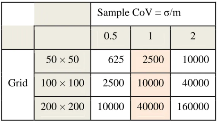
2* mesh. In case of a sample coefficient of variation

CoV M equal to 1, the specific volume coincides with the size of the mesh, and so with the inverse of the classical density of points in space, that is 1 point per mesh. A smaller sample CoV makes it smaller, a larger sample CoV makes it larger. In Table 2, we can see that the specific volume (in two dimensions) is the same with a sample CoV of 1 and a grid of 100 × 100, a CoV of 0.5 and a grid of 200 × 200 or a CoV of 2 and a grid of 50 × 50.

In the particular case of a grid which is large compared to the structure, a simple formula also exists for the specific volume. Following Matheron (1971), the estimation variance of a domain V estimated by N datapoints can be approximated by:

2 2 ( ) | |

1

( )

E V V

C h dh

N

 







where C(h) is the covariance function with 2

(0)

C  . The sampling density variance and the specific volume can be deduced:

1 2 3 4 5 6 7 8 9 10 11 12 13 14 15 16 17 18 19 20 21 22 23 24 25 26 27 28 29 30 31 32 33 34 35 36 37 38 39 40 41 42 43 44 45 46 47 48 49 50 51 52 53 54 55 56 57 58 59





2 2 ( ) | |

| |

)

E V V

v

A













2 2

| |

)

o V

v

A

M







They are proportional to the difference between the mesh size |v| = |V |/N and the integral

range 2

( )

C h dh A







, i.e. the volume characterizing the spatial structure (Chilès and Delfiner, 2012).

2.3.1 A toy example

The following toy example illustrates the interest of the concept of sampling density variance and of specific volume, in the context of optimal sampling. Consider a deposit with constant rock density, subdivided into different zones i = 1, …, n, each having its own volume V_i, tonnage T_i, metal Q_i, grade Z_i = m_i (the variogram of the point support grade within zone i is assumed to be a pure nugget effect i

2_{). How to allocate a given number N of samples at}

best, i.e. minimizing the global metal estimation variance?

Whatever the numbers N_i, the estimation variance of Z_i from N_i samples is



i2

N

i, the

sampling density variance (2) within zone i is Vi



i2

N

i , so is proportional to

2

i i i

T



N

, while the estimation variance of Q_i is

T

i2



i2

N

i. Hence the estimation variance of i

i Q



Q is 2 2 2 i i e Q i i T N   



The minimum of this quantity, with respect to the Ni given that their sum is N, gives the optimal N as the solution of the system:

1 2 3 4 5 6 7 8 9 10 11 12 13 14 15 16 17 18 19 20 21 22 23 24 25 26 27 28 29 30 31 32 33 34 35 36 37 38 39 40 41 42 43 44 45 46 47 48 49 50 51 52 53 54 55 56 57 58 59 60

i i i T i N  _  

where µ is a Lagrange parameter. The optimal N_i is found to be proportional to T_i_i : the larger the zone and the higher the standard deviation of the grade in this zone, the larger the number of samples in it. The optimal estimation variance of Zi from Ni samples is

proportional to



_i

T

_i . The optimal estimation variance of Q_i is proportional to

T

_i



_i. The optimal sampling density variance (2) within zone i is proportional to _i. And finally the

optimal specific volume (3) is proportional to



i

m

i2.

As could be expected, sampling density variance and specific volume do not depend on the zone extension. Classification of resources based on sampling density variance would ignore the level of the grades and would favor parts with lower variability (even if these are poorer due to a global proportional effect). In the current case of a proportional effect of the type "



_i

m

_i constant", the optimal specific volume is proportional to

1

m_i : the classification based on specific volume will favor parts where the mean is larger, which is satisfactory.

2.3.2 Example (regular sampling pattern)

The thickness of a mineralized layer has a mean of 10 m, a sample point variance of 10, and a variogram equal to 1 nugget(h) + 9 spherical (h/200 m). The extension variance of a

100 m × 100 m block by its center equals 2.69, so that for a 100 m × 100 m grid, the sampling density variance (2) is 26,900 m 4, and the specific area (specific volume (3) in two

dimensions) 269 m 2_{. A similar computation shows that the specific area would be reduced to}

46 m 2 for a 50 m × 50 m grid, for instance.

1 2 3 4 5 6 7 8 9 10 11 12 13 14 15 16 17 18 19 20 21 22 23 24 25 26 27 28 29 30 31 32 33 34 35 36 37 38 39 40 41 42 43 44 45 46 47 48 49 50 51 52 53 54 55 56 57 58 59

Now another issue is whether this 100 m × 100 m sampling is better, or not, than a 70 m × 70 m sampling in a similar deposit, where the thickness has a mean of 8 and a variogram equal to 6 nugget(h) + 6 spherical (h/200 m) (Fig. 2). Hence the nugget is higher, but the sampling is finer. Interestingly the sampling density variances (2) derived from the normalized variogram (sill set to 1) are quite close: 2690 in the first case, 2680 in the second one. However the sill is higher in the second case, so that the sampling density variance (2) is slightly higher (32,100 m 4 against 26,900 m 4). If additionally we take into account the means, the sampling is nearly twice less good in the second case, with a specific area (3) of 502 m2 against 269 m2. The finer sampling is not sufficient to compensate for the larger nugget component and, above all, the lower mean. As will be seen in the next paragraph (Eq. 5), we can deduce that, for instance, the 5% CoV area (area over which the mean thickness has a coefficient of variation of 5%) must practically reach 200,000 m2, while it is

only108,000 m2 in the first case.

2.3.3 Use of specific volume

The sampling density variance, or its simpler version the specific volume, can be used to characterize a regular sampling pattern with respect to the variogram. After that, the sampling density variance can be used to approximate the estimation variance of the regionalized variable over a volume V, typically a multiple of the mesh:

2 sampling density variance

( )

| |

E V

V

 

or to determine |V| having a given estimation variance _E2:

2

sampling density variance | | E V   1 2 3 4 5 6 7 8 9 10 11 12 13 14 15 16 17 18 19 20 21 22 23 24 25 26 27 28 29 30 31 32 33 34 35 36 37 38 39 40 41 42 43 44 45 46 47 48 49 50 51 52 53 54 55 56 57 58 59 60

Similarly the specific volume

V

₀( sampling density variance

M

2

)

can be used to directly obtain the coefficient of variation CoV_E/M corresponding to the estimation of the variable on a volume V: | | | | o V CoV V  ₍₄₎

or to determine |V| corresponding to a given CoV:

0 2

CoV

V

V  (5)

Hence, having characterized the sampling pattern by its specific volume, it is possible to relate volumes to their CoV. In term of mineral resource classification, V could be chosen as the volume to be mined in order to ensure the production in a given period, while thresholds on CoV would be used to categorize the resources. Note that the CoV used here is a nominal CoV, computed from the global mean M and the mean variogram. In practice the global mean M should be computed from the same data that are used to compute the variogram.

2.4 Case of an irregular sampling pattern

In the previous cases, the grid was supposed to be regular, either over the whole deposit, or over a part of deposit. But there are situations where the sampling pattern is not regular, typically when exploration is made by fans of holes. Often fans of holes are drilled within regularly spaced vertical sections, but the spatial density of data within each section is higher where the holes are close together, and smaller away from this. Then it may be important to make the distinction into parts that are more or less densely explored.

1 2 3 4 5 6 7 8 9 10 11 12 13 14 15 16 17 18 19 20 21 22 23 24 25 26 27 28 29 30 31 32 33 34 35 36 37 38 39 40 41 42 43 44 45 46 47 48 49 50 51 52 53 54 55 56 57 58 59

Here it is useful to make a parallel between the spatial sampling density variance, or even more the specific volume, and the inverse of the classical density of points in space, which is also a volume. From a simple physical point of view, the density of points in a given volume is the number of points within it, divided by the volume. So its inverse is the average volume occupied by one point. It is equal to the mesh size in the case of a regular grid. This physical point of view can be adopted for each part of a domain, in particular when the density of the points varies from one part to the other. However things are different when the density of points varies within the domain but without any a priori partitioning.

In that case, the density of points, supposed to vary within the domain, will rather be subject of local estimation, using a moving window or a more sophisticated kernel function (of course there is a question of scale here, as the result depends on the chosen window size). The

situation is very similar in our case, with the main difference that our sample points are associated with values of the regionalized variable, so that their influence in the spatial density should depend on the variogram. For instance, two close sample points should count differently whether the variogram contains a nugget effect or not. Hence it is proposed to measure the local density of sample points using the previously developed spatial sampling density variance (and the associated specific volume). This requires choosing a moving window that will capture inner samples. In mining exploration, even when the sampling pattern is irregular, holes are drilled in a systematical way, respecting directionality of

sections and lines, and the use of parallelepiped windows, i.e. superblocks, is appropriate. The size of the window must be chosen so that it includes a local but representative distribution of inner samples. Having chosen the superblock, one must compute its estimation variance when estimated by its inner samples. This can be done using a "superkriging", i.e. a kriging of

1 2 3 4 5 6 7 8 9 10 11 12 13 14 15 16 17 18 19 20 21 22 23 24 25 26 27 28 29 30 31 32 33 34 35 36 37 38 39 40 41 42 43 44 45 46 47 48 49 50 51 52 53 54 55 56 57 58 59 60

superblocks. Multiplying by the superblock volume gives the sampling density variance, and a further division by the squared mean gives the specific volume.

The superblock (the moving window) in the case of an irregular sampling pattern has the same role as big blocks set on the mesh, in the case of regular sampling. Both are usually much bigger than the usual blocks of the block model of the deposit. These smaller blocks are more appropriate to follow bodies with irregular geometries and to design mining projects. Moving the superblock window at the center of each block of the block model results in a map at this resolution (but the result at one location does not depend on the size of the small block). Having mapped the sampling density (or the specific volume), it is possible to make the distinction between more homogeneous domains that are sampled with different sampling densities, i.e. different levels of confidence. An average sampling density may then be

computed within such a domain, as the mean of the sampling density variances.

2.4.1 Example (irregular sampling pattern)

The concept is illustrated here on a porphyry copper deposit. This deposit has been sampled with fans of holes located within parallel sections spaced every 50 m. Superkriging was performed for each of the 10 m × 10 m × 10 m blocks of the block model. First,

50 m × 50 m × 50 m superblocks were used. However this resulted into envelops around each hole, since the distance between holes often exceeds 50 m (Fig. 3A). Satisfying results were obtained with 150 m × 150 m × 50 m superblocks, without any smoothing post-process (Fig. 3B). Homogeneously sampled domains can be drawn from such a map.

Having characterized in this way the spatial sampling within the deposit, this can be exploited to characterize resources given an assumption on the production volume (or more exactly the

1 2 3 4 5 6 7 8 9 10 11 12 13 14 15 16 17 18 19 20 21 22 23 24 25 26 27 28 29 30 31 32 33 34 35 36 37 38 39 40 41 42 43 44 45 46 47 48 49 50 51 52 53 54 55 56 57 58 59

gives a grade CoV of 4.7% for an annual production of 2.7 Mm3 _{(i.e. 7 Mt at 2.6 density), or a}

twice larger CoV (9.4%) on the corresponding quarterly production.

3 Discussion

The aim of this paper was to propose a concept to measure the spatial sampling density of a regionalized variable. The proposed spatial sampling density variance, derived from the concept of estimation variance, is additive, in the sense that its value for a big volume is the average of its values over parts dividing the volume. This requires parts having uncorrelated errors when estimating each of these by its inner samples. In the case of a regular sampling pattern within a big volume, this sampling density variance is constant and characterizes the pattern, depending on the variogram, not on the big volume. It thus allows comparing different sampling patterns within a given domain, or even sampling patterns on domains having different variograms. A variant of the sampling density variance, the specific volume, facilitates the measure and the comparison, by taking into account the mean of the variable in addition to its variogram.

The sampling density variance can be computed from big blocks corresponding to the mesh in the case of a regular grid. In the case of an irregular pattern, it can be computed from a

moving superblock, and then be mapped in order to make the distinction between domains with different spatial sampling densities. Compared to the common tools of geostatistics, the sampling density variance (and the associated specific volume) is a flexible substitute for the classical global estimation variance in the case of a regular grid, and otherwise provides a local measure of estimation variance that is not be dependent on the size of the block from the block model (but it depends on the moving superblock, just like the estimation of a local density of points in space depends on the moving window used). It proposes a description of

1 2 3 4 5 6 7 8 9 10 11 12 13 14 15 16 17 18 19 20 21 22 23 24 25 26 27 28 29 30 31 32 33 34 35 36 37 38 39 40 41 42 43 44 45 46 47 48 49 50 51 52 53 54 55 56 57 58 59 60

the sampling efficiency of a deposit, or within a deposit, which only depends on the spatial distribution of sample points, and on the mean and variogram of the variable.

This description can be used as an input for mineral resources classification in a geostatistical perspective. In particular the specific volume can be used to make a direct link between a nominal volume to be mined in a given period and its coefficient of variation. While conditional simulation is able to provide the uncertainty within a given delineated volume, taking into account the particularities of local data and local proportional effects, our concept only requires nominal volumes. It cannot replace conditional simulation to assess the

uncertainty of next quarterly production, but appears as a simple and flexible way to measure objectively the level of sampling within a deposit, even at the first stage of systematic

sampling (inferred resources).

As mentioned at the beginning, the concepts developed in this paper originated from mineral resources classification. However, the spatial sampling density variance proposed here appears as a new concept in geostatistics in general, not only in mining geostatistics. By measuring the level of sampling of a regionalized variable per se rather than at a given support, it enables to assess, map, and combine uncertainties over space.

4 Conclusion

The spatial sampling density variance of a regionalized variable in a domain is a measure of the spatial sampling density in this domain. When the domain is divided into parts, estimated from inner samples and having uncorrelated errors, the sampling density variance over the domain is the average of its values on the different parts. Thanks to this additivity property, the sampling density variance offers a way to combine uncertainties in space. In the case of a

1 2 3 4 5 6 7 8 9 10 11 12 13 14 15 16 17 18 19 20 21 22 23 24 25 26 27 28 29 30 31 32 33 34 35 36 37 38 39 40 41 42 43 44 45 46 47 48 49 50 51 52 53 54 55 56 57 58 59

homogeneous sampling pattern, the spatial sampling density variance is constant within the domain. In the case of an intrinsic variable, it depends on the variogram and on the sampling pattern, not on the domain extension. The spatial sampling density variance, or its variant, the specific volume, allows comparing different sampling patterns, in one domain or in several domains, having possibly different spatial structures. In case of an irregular sampling pattern, it can be mapped and allows distinguishing areas having a different sampling density. The specific volume is very similar to the inverse of the classical density of points in space, but depending on the spatial structure.

While common tools of geostatistics can provide the confidence on the estimation of a sampled variable on defined volumes, the present concept provides the level of confidence due to the density of spatial sampling. In the context of mineral resources classification, it can be used as a first step, to provide an objective description of the sampling effort throughout a deposit, enabling comparison between different domains or deposits. This first step may be further used to classify resources based on expected production volumes.

Acknowledgements

The authors are grateful to Codelco (Felipe Celhay) and Vale (in particular Celeste Queiroz and Leandro Jose Oliveira) for their support in this research. Mapping the specific volume has been made possible thanks to a "Superkriging" plugin developed for Geovariances Isatis software.

References

Chilès J-P, Delfiner P (2012) Geostatistics: Modeling Spatial Uncertainty, 2nd _{edition. New}

York. John Wiley & Sons, 731

1 2 3 4 5 6 7 8 9 10 11 12 13 14 15 16 17 18 19 20 21 22 23 24 25 26 27 28 29 30 31 32 33 34 35 36 37 38 39 40 41 42 43 44 45 46 47 48 49 50 51 52 53 54 55 56 57 58 59 60

Emery X, Ortiz JM, Rodríguez J J (2006) Quantifying Uncertainty in Mineral Resources by Use of Classification Schemes and Conditional Simulation, Mathematical Geology 38(4): 445-464

Geovariances (2012) Drill Hole Spacing Analysis, white paper, http://www.geovariances.com, 8

JORC (2012) The JORC code, AusIMM, 44

Journel AG, Huijbregts CJ (1978) Mining geostatistics. London. Academic Press, 600

Matheron G (1971) The theory of regionalized variables and its applications. Fontainebleau. Cahiers du Centre de Morphologie Mathématique 5. Ecole des Mines de Paris, 212

Rivoirard J (2013) A geostatistical measure for the spatial sampling of a deposit, Proceedings of 36th APCOM Conference, Brazil, pp 209-215

Sans H (2004) Resource risk characterisation, technical paper, Omega Geo-Consulting Pty Ltd, www.OmegaGeo.com, 1

Silva DSF, Boisvert JB (2014) Mineral resource classification: a comparison of new and existing techniques, The Journal of The Southern African Institute of Mining and Metallurgy, 114: 265-274 1 2 3 4 5 6 7 8 9 10 11 12 13 14 15 16 17 18 19 20 21 22 23 24 25 26 27 28 29 30 31 32 33 34 35 36 37 38 39 40 41 42 43 44 45 46 47 48 49 50 51 52 53 54 55 56 57 58 59

Tables captions

Table 1: Approximation of the estimation variance of a block subdivided into sub-blocks, each informed by 1, 2 or 3 samples (linear variogram γ(h) = |h|).

Table 2: Specific volume in the case of a square grid and a pure nugget effect.

Figures captions

Figure 1. (A) square grid; (B) a big 100 m × 200 m block, divided into six 100 m × 33 m blocks with 1 sample in each.

Figure 2. Which is better: (A) a 100 m × 100 m sampling of a thickness with mean 10 m and variogram equal to 1 nugget(h) + 9 spherical (h/200 m), or (B) a 70 m × 70 m sampling of a thickness with mean 8 and variogram equal to 6 nugget(h) + 6 spherical (h/200 m)?

Figure 3. Specific volume (in m 3) computed from (A) a 50 m × 50 m × 50 m superblock, (B) a 150 m × 150 m × 50 m superblock (vertical cross-sections).

1 2 3 4 5 6 7 8 9 10 11 12 13 14 15 16 17 18 19 20 21 22 23 24 25 26 27 28 29 30 31 32 33 34 35 36 37 38 39 40 41 42 43 44 45 46 47 48 49 50 51 52 53 54 55 56 57 58 59 60

Table 1

estimation variance

from six 100 m × 33 m blocks 2.97 from three 100 m × 67 m blocks 3.51 from two 100 m × 100 m blocks 3.80 of the 100 m × 200 m block (true) 4.15 1 2 3 4 5 6 7 8 9 10 11 12 13 14 15 16 17 18 19 20 21 22 23 24 25 26 27 28 29 30 31 32 33 34 35 36 37 38 39 40 41 42 43 44 45 46 47 48 49 50 51 52 53 54 55 56 57 58 59

Table 2

Sample CoV = σ/m 0.5 1 2 50 × 50 625 2500 10000 Grid 100 × 100 2500 10000 40000 200 × 200 10000 40000 160000 1 2 3 4 5 6 7 8 9 10 11 12 13 14 15 16 17 18 19 20 21 22 23 24 25 26 27 28 29 30 31 32 33 34 35 36 37 38 39 40 41 42 43 44 45 46 47 48 49 50 51 52 53 54 55 56 57 58 59 60

Fig1

o o o o o o o o o o o o o o o o (A) (B) o o o o o o 1 2 3 4 5 6 7 8 9 10 11 12 13 14 15 16 17 18 19 20 21 22 23 24 25 26 27 28 29 30 31 32 33 34 35 36 37 38 39 40 41 42 43 44 45 46 47 48 49 50 51 52 53 54 55 56 57 58 59

Fig2

(A) (B) 1 2 3 4 5 6 7 8 9 10 11 12 13 14 15 16 17 18 19 20 21 22 23 24 25 26 27 28 29 30 31 32 33 34 35 36 37 38 39 40 41 42 43 44 45 46 47 48 49 50 51 52 53 54 55 56 57 58 59 60

Fig3

1 2 3 4 5 6 7 8 9 10 11 12 13 14 15 16 17 18 19 20 21 22 23 24 25 26 27 28 29 30 31 32 33 34 35 36 37 38 39 40 41 42 43 44 45 46 47 48 49 50 51 52 53 54 55 56 57 58 59