State history tree: an incremental disk-based data structure for very large interval data

(1)

Titre:

Title

:

State history tree : an incremental disk-based data structure for

very large interval data

Auteurs:

Authors

:

Alexandre Montplaisir-Gonçalves, Naser Ezzati-Jivan, Florian

Wininger et Michel R. Dagenais

Date: 2013

Type:

Communication de conférence / Conference or workshop item

Référence:

Citation

:

Montplaisir-Gonçalves, A., Ezzati-Jivan, N., Wininger, F. & Dagenais, M. R. (2013, septembre). State history tree: an incremental disk-based data structure for very

large interval data. Communication écrite présentée à International Conference

on Social Computing (SocialCom 2013), Alexandria, VA, USA (9 pages). doi:10.1109/socialcom.2013.107

Document en libre accès dans PolyPublie

Open Access document in PolyPublie

URL de PolyPublie:

PolyPublie URL: https://publications.polymtl.ca/2983/

Version: Version finale avant publication / Accepted version_{Révisé par les pairs / Refereed} Conditions d’utilisation:

Document publié chez l’éditeur officiel

Document issued by the official publisher

Nom de la conférence:

Conference Name: International Conference on Social Computing (SocialCom 2013)

Date et lieu:

Date and Location: 2013-09-08 - 2013-09-14, Alexandria, VA, USA

Maison d’édition:

Publisher: IEEE

URL officiel:

Official URL: https://doi.org/10.1109/socialcom.2013.107

Mention légale:

Legal notice:

reprinting/republishing this material for advertising or promotional purposes, creating new collective works, for resale or redistribution to servers or lists, or reuse of any copyrighted component of this work in other works.

Ce fichier a été téléchargé à partir de PolyPublie, le dépôt institutionnel de Polytechnique Montréal

This file has been downloaded from PolyPublie, the institutional repository of Polytechnique Montréal

(2)

State History Tree : an Incremental Disk-based Data Structure for

Very Large Interval Data

A. Montplaisir-Gon¸calves

N. Ezzati-Jivan

F. Wininger

M. R. Dagenais

alexandre.montplaisir, n.ezzati, florian.wininger, michel.dagenais @polymtl.ca

August 9, 2013

Abstract

In this paper, we propose the State History Tree, a disk-based data structure to manage large streaming interval data. The State History Tree provides an ef-ficient way to store interval data on permanent stor-age with a logarithmic access time. The disk-based structure ensures that extremely large data sets can be accommodated. The State History Tree stores in-tervals in blocks on disk in a tree organization. Un-like other interval management data structures Un-like R-Trees, our solution avoids re-balancing the nodes,

speeding up the tree construction. The proposed

method is implemented in Java, and evaluated using large data sets (up to one terabyte). Those data sets were obtained from the state intervals computed from system events traced with the LTTng kernel tracer. The evaluation results demonstrate the performance and efficiency of the method, as compared with other solutions to managing huge interval data sets.

1 Introduction

Several methods have been introduced in the litera-ture to manage data intervals within different appli-cations and database systems. However, managing incrementally-arriving data (e.g. data streams com-ing from network or system traces, phone call logs, financial transactions, and so on) introduces some performance challenges and is required in many ap-plications.

In this paper, we present the State History Tree to manage a large set of interval data that arrive in-crementally and are time ordered. The State His-tory Tree is a data structure to store intervals, and is optimized for block devices like rotational disks. Most existing tree structures proposed in the litera-ture to deal with intervals are currently optimized for memory storage (typically binary trees, with a large number of levels). Other structures like B-trees are well optimized for disk storage. Unfortunately, they deal with single values, not intervals. The State His-tory Tree presented here borrows concepts from both those types of structures, and allows storing a large number of intervals on disk, while allowing them to be queried in an efficient way.

We have used the State History Tree to manage intervals of system state values, coming from trace data generated by the LTTng tracer [1]. The State History tree stores data in logical nodes which are

mapped to a single or multiple disk blocks. Each

node may contain numerous intervals. Each interval contains the start and end points (timestamps), a key and a value. The key can be a single value or a multi-part value. Integer and String data types are supported for the value.

The interval data is stored in tree nodes in memory while it arrives incrementally. When a node is full, it is committed to disk, and another node is created and added to the tree. This solution avoids re-balancing tree nodes and results in a very fast tree construc-tion. Also, although the data is stored on disk, it

(3)

still provides a fast access time (logarithmic). The rest of the paper is organized as follows: we first take a look at different structures used to manage intervals, then we present the details of our solution. Finally, we will discuss the implementation of our solution and compare its performance with other data structures like the R-Tree and PostgreSQL/PostGIS.

2 Related Work

Several methods have been introduced in the litera-ture to store and manage interval data. Here, we will review several structures and compare them to our use cases.

Segment tree

The segment tree is a binary tree (two children per node) and, as described in [2], is well-known to store intervals in one dimension. It is actually a balanced tree, with a static structure, where a tree node may correspond to several intervals. This implies that the tree will usually be deep. The segment tree is there-fore more appropriate for main memory storage.

When a hard disk is used, the number of non-consecutive blocks to read is the main concern. In-deed, the disk head must be repositioned before each read, adding the positioning time to reading time. For this reason, disk based trees typically use large tree nodes and a large number of children at each node, leading to a shallow tree. In that case, each node fits in a disk block and for a typical access, from the root to a leaf in the tree, few blocks need to be read.

R-Tree and its Variants

The R-Tree [3] and its variants like R+ Tree [4] and R* Tree [5] are widely used to store spatial informa-tion, usually in two or three dimensions, but they can also be used in a single dimension. All data stored in the tree are completely contained at the leaf level. Each additional level only increases the ”mesh”. As the tree is not binary, they are better than segment trees for disk storage.

The R* Tree meanwhile is closer to the original R-Tree, but offers a more complex insertion method, which uses heuristics to ensure that each leaf node is as balanced as possible. Queries on R* Tree are generally faster, with a better nodes arrangement.

The principle behind the Hilbert R-Tree [6], an-other variant of the R-Tree, is to use the Hilbert curve

1 _{on the values to be stored to define the nodes of}

the tree. This results in a very compact tree that is well suited for interval queries. The Hilbert R-Tree is more suitable for high-dimensional data sets. There-fore it is probably not the ideal structure to store single dimensional time information.

Finally, another potentially interesting variant is the Historical R-tree [7]. It stores time changing in-formation. The method used is to keep a separate R-Tree for each time unit. Identical nodes from one tree to another will not be copied, but only a refer-ence to the first node of the series.

Nevertheless, we can expect some space overuse. If only one value changes in a node, the full node must be copied in the next tree. In addition, the creation of a tree per time unit may become very costly for trace analysis, where the base unit is typically the nanosecond.

B-Trees

The B-Tree, first introduced by Comer [8], suggests another tree organization that can be conducive to disk storage. The nodes are usually large, and have many children. This leads to shallow trees, so a few different nodes will be read during the exploration of a single branch.

B-Trees are balanced structures with a configurable node size (number of entries contained within). Each intermediate node contains an array of key and child

pairs. All the values in a child (and its recursive

children) will be located between the previous and

current key. The tree should be rebalanced when

adding or removing nodes. The criteria for adding or removing a node can be configured. For example, one may decide to split a node when it becomes full, but to merge adjacent nodes only if the resulting node

(4)

would be 50% full or less.

The use of B-Trees for a file or database systems is interesting, but the use of COW (Copy-on-Write) makes it more exotic and difficult to apply to disk storage of intervals.

7

Hybrid structures

In this final subsection, we introduce more

application-specific structures. We first studied the Interval B-tree of [9]. It proposes the use of three data structures, all contained in memory, to store in-tervals. The three components are a B+ Tree, two linked lists, and a binary search tree. The first two contain information relative to the intervals them-selves, and the third serves as an index to speed up queries. To increase the capacity of the structure, the B+ tree could possibly be saved to disk and re-main relatively effective. However this is not the case for the linked lists or the binary tree. Moreover, as the content of these structures grows with the num-ber of inserted intervals, we would still be limited by memory space.

We then looked at the Relational Interval Tree,

or RI-Tree [10]. Their solution is actually an

ex-ternal addition to a relational database. They use an in-memory structure for intervals, which enables the optimization of queries that will ultimately be sent to the database. Their work is interesting, and can be used to extend the functionality of a standard RDBMS to support efficiently interval data and in-tersection queries. However, as will be seen in the results section, using a general purpose database in-curs a significant performance penalty.

Then, the MV3R-Tree [11] caught our attention. The Multi-Version 3D R-Tree is actually a MVR-Tree (Mutli-version R-MVR-Tree) coupled with R-MVR-Trees in three dimensions. However, as can be expected, they use the R* Tree algorithm for separating nodes, since it generally gives more efficient trees. The authors say that by using these structures in parallel, they can respond to two common types of queries on spa-tial data structures: the MVR-Tree is ideal for point queries applications, but the 3D R-Tree will be bet-ter for inbet-terval queries. In our case, we are mostly

interested in point queries, we will thus focus on the MVR-Tree.

A MVR-Tree is an alternative to the Historical R-Tree, mentioned earlier, for storing the evolution over time of a regular R-Tree. Instead of creating a new tree for each time unit, as with the Historical Tree, the MVR-tree uses the time as third dimen-sion. Thus, it saves considerable space compared to the Historical Tree. This makes it an excellent struc-ture for recording the evolution of the 2D position of objects through time, for example.

Although this kind of structure is very interesting, it probably does not lend itself well to store interval data, where our only dimension is time. It would also be incorrect to consider such attributes as another dimension, since we have no guarantee that there are logical connections between them (this is not because a given attribute has changed that his neighbours are likely to change). In addition, the values of intervals are mostly qualitative, so you can usually not even talk about values ”closer” to each other.

Finally, we studied the External Interval Tree [12]. Of all the solutions proposed so far, it seemed the closest to our application. The authors define the Weight-balanced B-tree, or B-tree swayed by the weight. In this variant, it is not the number of chil-dren which is the criterion of re-balancing, but the weight assigned to each sub-branch. The weight is determined by the total number of items located in the sub-branch, not the number of nodes in the next level.

This can help to better manage the re-balancing steps of the structure on disk. Indeed, since we are on disk, we should minimize rebalancing. The main sec-tion of the paper describes ways to perform these re-balancing without sacrificing too much performance. The techniques are very clever, but unfortunately it would not help us much for interval storage. As we will see in the next section, our intervals are already sorted when inserted, it is thus easier to design a structure that never needs to be rebalanced.

Nonetheless, maintaining a constant depth for all

tree branches is desirable. Indeed, if the tree has

the same number of nodes in all its branches, the query time will be essentially the same, regardless of the location targeted. It also controls the worst-case

(5)

behavior, a desirable feature for our application.

3 Design of the History Tree

In this section, we propose the State History Tree, a data structure to store intervals optimized for block devices. It is by no means balanced, there is no con-cept of re-balancing the tree. To clarify our use cases, we introduce the following assumptions on the inter-vals to be stored in this structure:

• The time is used to define interval borders. How-ever, other information can be used here as well (e.g. physical location).

• The interval lengths are short on average, rela-tive to the total length of the structure (in our case, the trace).

• The intervals will be inserted in sorted order of end time.

The third assumption is particularly important in the design of the history tree. If the intervals are inserted strictly in chronological order, without ever inserting ”in the past”, this means that the struc-ture will never have to be rebalanced. It could also be built incrementally (where the completed portion of the structure does not change thereafter). In the following, we discuss the various components of the State History Tree to understand how the tree is built and how it can be used later.

3.1 Intervals

Intervals are the basic units of the history tree. Each interval consists of a key, a value, a start time and an end time. The start and end times are the bounds of the interval, and represent a period for which a given attribute has a given value. These times must be in-teger values and represent times in minutes, seconds, microseconds or even nanoseconds.

The key is an integer and may come from another tree or structure to explain what entityattribute has the associated value for the specified interval.

The value is the actual payload of the interval, rep-resenting the exact value of the given key in the cor-responding time duration. For example, in the con-text of the execution trace on a multicore system, sample keys and associated values for different inter-vals could include: (PID of current process on CPU0, 1534), (command name of process 1534, ”bash”), (ex-ecution state of process 1610, BLOCKED ON IO), etc.

3.2 Tree Nodes

The nodes of the State History Tree are the direct containers for intervals. Thus, in addition to the in-tervals contained within, each Node stores the fol-lowing fields: sequence number, start time, end time, pointer to parent node, pointers to children, children start times, list of contained intervals.

When the tree is built, sequence numbers are at-tributed sequentially to nodes as they are created. They give a unique ”key” to each node, which is used to locate it in the disk file. The Start time and End time are simply equal to the earliest and latest timestamps, respectively, found amongst all the in-tervals it contains. Each node also keeps an array of timestamps, representing the start times of its chil-dren nodes. When we navigate the tree downwards using a target time value, we want to be able to select the correct child node without having to read all of them from disk. Having the ”borders” of each child also stored in the parent node allows us to do so.

3.3 Blocks

Nodes and their contents are written to disk as ”blocks”. Each block has a fixed-size, which is user-specified at construction time and stored in the file header. Each block contains a fixed-size header, a Data section and a Strings section. The header con-tains global information about the associated node.

Each interval belonging to this node will have an entry in the Data section. Each entry has a fixed size, which allows random access to the entries, for exam-ple to perform a binary search. The number of such entries however varies from node to node depending on the size needed by the Data and Strings sections.

(6)

The Strings section is used to store variable-length arrays of bytes. Because of the variable size of its elements, the Strings section starts at the end of the node and grows backwards. The entries in the Data section can optionally refer to an entry in the Strings section.

The size of each block is determined in advance. Nodes therefore have a limit on the number of in-tervals they may contain. This limit also depends on the type of interval contents, since interval values with strings can be of variable size.

As a node grows, the end of the Data section and the start of the Strings section will get closer, up to the point where there will not be enough space between the two and an interval insertion will fail. Therefore, when a node is ”full”, it has reached its maximum size, and no more interval can be inserted from now on. When this happens, the node is saved to disk, and no more insertions will be allowed.

3.4 Tree Construction

So far, we have seen different parts of the history tree. Let’s see how they fit together to form a tree. The State History Tree is based on the fact that inser-tions will be done sequentially, with intervals inserted sorted by ascending End times.

The tree supports inserting elements farther in the past, but doing it often can lead to more imbalance (higher level nodes being filled faster than leaves), and at worst the tree would degenerate into a linear list of nodes.

When a node is full (when there is no more room in the block on disk), it gets ”closed”, and the latest End time found in the interval it contains becomes

the node’s End time. A new sibling node is then

added to its right. If the maximum number of nodes is reached in the parent, a new sibling is added to the parent, and so on up to the root node.

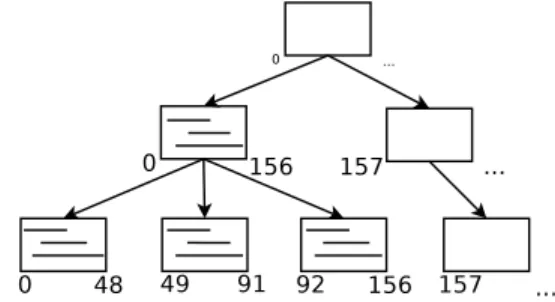
The following list of figures shows an example of a tree that gets built from scratch. The small numbers represent start times and end times for each node.

Figures 1 and 2 show the different construction phases of the history tree.

The construction algorithm starts with a single empty node, and with its start time equal to the start time given to the state history (we use 0 here). All inserted intervals are stored in this node.

When the node is filled, we mark it as ”full” and note the highest time among the existing interval

ends. We assign this time as the node’s own end

time. We now need to add a sibling node in which we can continue to insert the following intervals. A new root must also be added to connect the two sib-lings. The start time of the new sibling is the end time of the initial full node.

For future insertions, a choice must be made be-tween the right child node and the root node, since the left child node is full. We want to insert intervals in the lowest-level nodes as much as possible. This will only be permitted if the start time of the interval is greater than or equal to the start time of this node. In the example in Figure 1, if an interval with a start time of 50 needs to be inserted into the history, we can place it in the leaf node. On the opposite, a range with a start time of 20 cannot be placed there, so in this case the interval we will placed in the root node. Therefore, the root node used to store the intervals overlap its two children. It is here that the second assumption mentioned in the previous section comes in. Since the intervals are usually short, the majority of intervals enter the leaf nodes, and the root node will not fill too quickly. This assumption is required to obtain a large number of children nodes, and thus a shallow tree.

If, as we hope, the leaf node is filled first, a new leaf node will be added. As previously, we will close the previous node with the last time it contains, and assign this time as start time of the new node (Figure 1). For subsequent insertions, we choose between the new leaf node and the root node.

The insertion process continues until one of two things happen: the root node itself becomes ”full” in terms of intervals, or it reaches its maximum allowed number of children. In either case, we will close the root node.

If it is not already done, we also close the most recent leaf node with the same end time as its par-ent. The next step is to add a new sibling to the root node itself, and create a new parent root node.

(7)

Figure 1: Construction of the history tree

Whenever we create a new root node for the tree, we immediately create a complete branch, down to the leaf level. The start time of these new nodes, except for the new root node, will all be the same, and equal to the end time of the previous root node. We then end up with a situation like in Figure 2.

When there is no longer any new interval to insert, we simply point out that the history is completed. The highest end time in the tree is used as the final end time for all nodes in the right-most branch, and the completed history tree is marked as ”closed”.

3.5 Queries

Once closed, the history tree may be the target of queries to extract intervals at any timestamp. We saw in the previous section that during its construc-tion, only the rightmost branch can receive intervals and all other nodes are fixed and will not be changed. It would then be technically possible to run queries on a tree that is not closed, as long as we limit our-selves to the fixed part of the history.

The basic way to query the tree is to simply sup-ply a time point. A search will be started from the root node downwards, exploring only the branch that can possibly contain the given time point. Within each node, the algorithm iterates through all the in-tervals and returns only those intersecting the target time. If an input key is provided, then the algorithm stops as soon as it meets an intersecting interval cor-responding to the key of interest (we call this query ”ad-hoc”).

If no key is given, all intersecting intervals, with their key/value pairs and bounding times, are re-turned to the querying application (we call this a

”full query”). The ad-hoc queries return much less information, but are much faster on average than

full queries. We will see in the next chapter the

differences in performance between the two types of queries.

Figure 3 shows an example of a complete and closed off Tree, on which we run a query for time t = 300. In practice, the number of children per node is much higher. Here, we limited ourselves to two or three children to simplify the representation.

Figure 2: Root node is full (or max number of chil-dren reached), adding a new root node and a new branch

In the example shown in Figure 3, we assumed that the tree receives a request to return the intervals at time t = 300. The tree will explore the nodes shown in gray in the figure to find the necessary information.

4 Experimental Results

All experiments were performed on an Intel Core i7 920 @ 2.67GHz machine with 6 GB RAM using data gathered from LTTng kernel tracer. The pro-posed system is implemented as a Java library in the

(8)

Figure 3: Searching through the tree to get all inter-vals intersecting t = 300

Eclipse Tracing and Monitoring Framework (TMF,

an Eclipse plugin part of the Linux Tools project2).

The library is used to manage system states [13] ex-tracted from LTTng kernel tracer [1] for analyzing system runtime behavior. It has also been used to manage common states for generating abstract events [14] or handle system statistics [15].

4.1 Block sizes

The size of the blocks is configurable per tree. Smaller blocks will be filled faster, so the number of nodes and the number of levels in the tree will be larger. Accordingly, the number of read operations associated with a query will be larger. Larger blocks, on the other hand, require more time for each read operation and more processing to search for intersect-ing intervals. The optimal value is thus not obvious. Figure 4 shows the query time comparisons using different block sizes: 16KB, 64KB, 256KB, 1MB and 4MB.

The block sizes of 16KB to 256KB definitely seem to behave better for our traces. The 4MB block size seems inappropriate; the number of intervals to scan in each node becomes very large, which greatly slows down the queries.

Figure 5 shows the average time for full queries within very large inputs (for traces of 10 GB to 550 GB respectively). The test is conducted to evaluate the scalability with respect to the size of input data

2 http://www.eclipse.org/linuxtools/projectPages/ lttng/ 0 100000 200000 300000 400000 500000 600000 700000 800000 0 2000 4000 6000 8000 10000 12000

Time for a full query (

µ

s)

Size of the original Trace (MB) 16 KB 64 KB 256 KB 1024 KB 4096 KB

Figure 4: Full query time using different block sizes

0 50 100 150 200 250 10 100 1000 10000 100000 1e+06 Query Time (ms)

Size of the original Trace (MB) 32 KB Blocks

1 MB Blocks 4 MB BlocKs

Figure 5: Full query time using very large input data

that the history tree can support, and also to evalu-ate the query time for large input data. In the graph shown in Figure 5, the X axis is on a logarithmic scale. For the smallest traces, 32 KB blocks seem to offer the best performance. When the trace size exceeds 10 GB, however, 1 MB blocks are slightly better. Furthermore, query times are still very rea-sonable: about 150 ms for a full query and 2 ms for an ad-hoc query.

4.2 Comparison

with

other

data

structures

4.2.1 In-memory R-Tree

In this experiment, we compare our solution to R-Trees. To do so, an in-memory implementation of a R-Tree is selected. Also, we changed our solution to store data in memory instead of disk to be able to compare both solutions.

As can be seen in Figure 6, filling the R-Tree in memory is much longer than the history tree. The

(9)

0 50 100 150 200 250 300 350 0 100 200 300 400 500 600 700

History build time (s)

Size of the original Trace (MB) Full history tree Particial history tree Memory R−Tree

Figure 6: Comparison of construction time against R-Tree

reason is that a high amount of tree balancing is re-quired to build the R-Tree. Indeed, the construction of the State History Tree benefits from the property that the intervals arrive in sorted time order. How-ever, this is not the case for more generic structures like R-Tree, which must be constantly rebalanced. Other experiments show that the in-memory query time of the R-Tree is much better than our solution, as shown in Figure 7. 0 5000 10000 15000 20000 25000 0 100 200 300 400 500 600 700

Time for a full query (

µ

s)

Size of the original Trace (MB) Full history tree Particial history tree Memory R−Tree

Figure 7: Full query time, comparison of R-Tree and History Tree

In summary, the use of an R-Tree for interval data allows for very fast in-memory query time. Unfortu-nately, in-memory operation severely limit the allow-able history size, and the long construction time is problematic.

4.3 PostGIS

The next comparison is to use a database for storing the interval data. A ”spatial” database, like Post-GIS (an extension to PostgreSQL), can store

multi-dimensional information. Moreover, this database

stores its files on disk, supporting much larger data sets than the in-memory implementation of the pre-vious experiment. 0 500 1000 1500 2000 2500 3000 3500 20 30 40 50 60 70 80 90 100 110 120 130

Size of the Histoty tree (MB)

Size of the original Trace (MB) Full History Tree

PostGIS Database 77 225 344 820 2212 3300

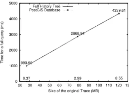
Figure 8: Comparison of disk usage against Post-greSQL/PostGIS 0 1000 2000 3000 4000 5000 20 30 40 50 60 70 80 90 100 110 120 130

Time for a full query (ms)

Size of the original Trace (MB) Full History Tree

PostGIS Database

0.37 2.99 8.55

990.90

2868.94

4339.61

Figure 9: Full query time, comparison of

Post-greSQL/PostGIS and History Tree

Figures 8 and 9 show the comparisons of disk space usage and full query time between the two solutions. While databases are generic mechanisms that can-not be expected to provide better performance than efficient special-purpose solutions, the maturity and emphasis on performance of the database field would suggest a modest penalty. It appears that for applica-tions with such large data sets, the overhead imposed by a generic database system remains very large, cre-ating much larger storage files and resulting in queries that cannot achieve the O(log n) behaviour of the State History Tree.

(10)

5 Conclusion

In this paper, we presented the State History Tree, an efficient data structure to store streaming interval data. The data structure uses a disk-based format to store the intervals and was tested for large data sets, up to hundreds of gigabytes.

This solution is implemented in Java in the Eclipse Tracing and Monitoring Framework, as a part of

Linux Tools Project3, and is publicly available. It is

used to store and manage the system states (modeled as interval data) gathered from large execution trace files. The LTTng tracer is used to generate input traces.

The evaluation of the proposed solution and its comparison with other approaches like R-Tree and PostgreSQL/PostGIS demonstrates the efficiency of the method, in terms of construction time, memory space usage as well as query access times.

References

[1] M. Desnoyers and M. Dagenais, “The lttng tracer: A low impact performance and behavior monitor for gnu/linux,” in Proceedings of the Ottawa Linux Symposium, vol. 2006, Citeseer, 2006.

[2] M. De Berg, O. Cheong, and M. Van Kreveld, Computational geometry: algorithms and applications. Springer-Verlag New York Inc, 2008.

[3] A. Guttman, R-trees: a dynamic index structure for spatial searching, vol. 14. ACM, 1984.

[4] T. Sellis, N. Roussopoulos, and C. Faloutsos, “The r+-tree: A dynamic index for

multi-dimensional objects,” pp. 507–518, 1987. [5] N. Beckmann, H. Kriegel, R. Schneider, and

B. Seeger, The R*-tree: an efficient and robust access method for points and rectangles, vol. 19. ACM, 1990.

3_{www.eclipse.org\/linuxtools\/}

[6] I. Kamel and C. Faloutsos, Hilbert R-tree: An improved R-tree using fractals. Citeseer, 1994. [7] M. Nascimento and J. Silva, “Towards

historical R-trees,” in Proceedings of the 1998 ACM symposium on Applied Computing, pp. 235–240, ACM, 1998.

[8] D. Comer, “Ubiquitous B-tree,” ACM Computing Surveys (CSUR), vol. 11, no. 2, pp. 121–137, 1979.

[9] C. Ang and K. Tan, “The interval B-tree,” Information Processing Letters, vol. 53, no. 2, pp. 85–89, 1995.

[10] H. Kriegel, M. P¨otke, and T. Seidl, “Managing

intervals efficiently in object-relational databases,” in Proc. 26th Int. Conf. on Very Large Databases (VLDB), pp. 407–418, Citeseer, 2000.

[11] Y. Tao and D. Papadias, “The MV3R-Tree: A spatio-temporal access method for timestamp and interval queries,” in Proceedings of the 27th VLDB Conference, 2001.

[12] L. Arge and J. S. Vitter, “Optimal external memory interval management,” SIAM Journal on Computing, vol. 32, no. 6, pp. 1488–1508, 2003.

[13] A. Montplaisir, “Stockage sur disque pour

acce`es rapide d’ attributs avec intervalles de

temps,” Master’s thesis, Ecole polytechnique de Montreal, 2011.

[14] N. Ezzati-Jivan and M. R. Dagenais, “A stateful approach to generate synthetic events from kernel traces,” Advances in Software Engineering, vol. 2012, April 2012. [15] N. Ezzati-Jivan and M. R. Dagenais, “A

framework to compute statistics of system parameters from very large trace files,” SIGOPS Oper. Syst. Rev., vol. 47, pp. 43–54, Jan. 2013.