HAL Id: hal-01963668
https://hal.inria.fr/hal-01963668
Submitted on 30 Sep 2019HAL is a multi-disciplinary open access
archive for the deposit and dissemination of sci-entific research documents, whether they are pub-lished or not. The documents may come from teaching and research institutions in France or abroad, or from public or private research centers.
L’archive ouverte pluridisciplinaire HAL, est destinée au dépôt et à la diffusion de documents scientifiques de niveau recherche, publiés ou non, émanant des établissements d’enseignement et de recherche français ou étrangers, des laboratoires publics ou privés.
wind instruments
Robin Tournemenne, Jean-François Petiot, Bastien Talgorn, Joel Gilbert,
Michael Kokkolaras
To cite this version:
Robin Tournemenne, Jean-François Petiot, Bastien Talgorn, Joel Gilbert, Michael Kokkolaras. Sound simulation-based design optimization of brass wind instruments. Journal of the Acoustical Society of America, Acoustical Society of America, 2019, 145 (6), pp.3795-3804. �10.1121/1.5111346�. �hal-01963668�
Robin Tournemenne,1 Jean-Franc¸ois Petiot,2 Bastien Talgorn,3 Jo ¨el Gilbert,4 and
Michael Kokkolaras3
1)Magique 3D Team, Inria Bordeaux Sud Ouest, 200 avenue de la vieille tour,
33405 Talence Cedex, Francea
2Ecole Centrale de Nantes, LS2N, UMR CNRS 6004, 1 rue de la No¨e,´
44321 Nantes Cedex 3, Franceb
3Department of Mechanical Engineering, McGill University, Montr´eal, QC H3A 0C3,
Canadac
4Laboratoire d’Acoustique de l’Universit´e du Mans, UMR CNRS 6613,
We present a method for optimizing the inner shape of brass instruments using sound
1
simulations. This study considers different objective functions and constraints
(represen-2
tative of both the intonation and the spectrum of the instrument) for a relatively large
3
number of design variables. A complete physics-based model, taking into account the
in-4
strument and the musician embouchure, is used to simulate permanent regimes of sounds
5
by means of the harmonic balance technique, the instrument being represented by its input
6
impedance. The design optimization variables are related to the geometrical dimensions of
7
the resonator. The embouchure’s parameters are varied during the optimization procedure
8
to obtain an average behavior of the instrument. The objective and constraint functions of
9
the optimization problem are evaluated using the physics-based simulation model, which is
10
computationally expensive. Moreover, the gradients of the objective and constraint
func-11
tions can be discontinuous, unavailable, or hard to approximate reliably. Therefore, we
12
employ a surrogate-assisted derivative-free optimization strategy using the mesh adaptive
13
direct search algorithm (MADS). One example of a B[ trumpet’s bore is used to
demon-14
strate the effectiveness of the design optimization approach: the obtained results improve
15
previously reported objective function values significantly.
16
a)[email protected]; b)[email protected]; c)[email protected]; d)[email protected];
I. INTRODUCTION
17
The development of innovative and higher-quality designs is crucial to the viability of musical
18
instrument manufacturers. Many prototypes are required to ensure that quality attributes such as
19
intonation, ease of emission, timbre, projection, etc. are adequate at each stage of the
develop-20
ment process. Numerical acoustics models may be helpful in shortening development cycles by
21
minimizing the manufacturing of costly prototypes. For example, in the case of brass instruments,
22
several studies propose the use of numerical modeling to predict quality and guide the design
23
process (Campbell,2004;Macaluso and Dalmont,2011).
24
The dominant physical quantity impacting the sound quality of a brass instrument is its input
25
impedance (cf. Figure 1). Input impedance is the frequency-dependent quotient of pressure and
26 0 200 400 600 800 1000 1200 1400 1600 1800 2000
frequency (Hz)
0 2 4 6 8 10 12 14|Z
|
(k
Ω
)
×1072 3
4
5
FIG. 1. Simulated input impedance Z of a B[ trumpet (magnitude), highlighting resonances 2, 3, 4, and 5 of the instrument
27 28
volume flow at the instrument entry plane, and, at first approximation, is the result of the
strument’s interior shape (the bore). Many works have focused on modeling input impedance,
30
e.g., (Causs´e et al.,1984).
31
The impact of input impedance on sound quality is acknowledged in (Campbell,2004), where,
32
in a first approximation attempt, playing frequencies are governed mainly by corresponding
33
impedance peaks (Eveno et al., 2014). Beyond influencing the instrument intonation, impedance
34
also determines an instrument’s timbre and playability, notably due to the height and bandwidth
35
of peaks.
36
With this in view, several researchers have used input impedance to design an instrument’s inner
37
shape using an optimization approach. Following Kausel’s successful reconstruction of a trumpet
38
bore using the Rosenbrock algorithm (Kausel,2001), Noreland optimized the instrument’s
intona-39
tion with a hybrid scheme for the input impedance model and shape constraints (Noreland et al.,
40
2010). Braden also optimized the intonation and the input impedance peak heights of a trombone
41
using a multi-modal input impedance model (Braden et al.,2009), while Macaluso optimized and
42
built a near-perfect harmonic trumpet (Macaluso and Dalmont,2011). Some studies investigated
43
the relationship between input impedance features and psycho-acoustic criteria: Poirson optimized
44
the trumpet using objective functions based on the input impedance and targets defined by
trum-45
pet players preferences (Poirson et al.,2007). Guillauteau looked for empirical relations between
46
playing frequencies and resonance frequencies to optimize clarinets (Guilloteau,2015).
47
However valuable, these works focused exclusively on instrument performance, neglecting a
48
crucial element in sound production: the musician embouchure. In particular, the studies of Eveno
49
et al. showed that the relationship between the resonance frequencies of the impedance and the
50
actual frequencies of the sounds played by musicians can vary significantly (Eveno et al., 2014).
Although the impedance of an instrument provides interesting information about sound quality,
52
prediction of “playability” and sound qualities of brasses based solely on impedance remains
dif-53
ficult.
54
A second approach is based on a holistic model of the physical phenomenon, coupling the
55
instrument and the musician embouchure, to produce sound simulations representative of the
in-56
strument quality. Using this approach, the authors integrate sound simulations in the optimization
57
process. These simulations are obtained from a physics-based model to account for the interaction
58
of the instrument with a virtual musician embouchure (Tournemenne et al., 2017). In a previous
59
study, the instrument’s intonation was optimized based on simulated playing frequencies (
Tourne-60
menne et al.,2017). Two examples were considered, optimizing 2 and 5 of the bore’s geometrical
61
parameters, respectively; results were quite encouraging.
62
The main objective of the present paper is to extend this new optimization paradigm in order to
63
assess both its potential and limitation. The two main novelties of this paper are the optimization
64
of criteria based on the instrument sounds spectra, and the inclusion of constraints in the problem
65
formulation. Three other contributions are noticeable: i) an improved version of the optimization
66
method has been implemented, ii) a new solver is introduced, and iii) the performance limits of the
67
optimization method are tested by considering 10 geometrical variables of the bore. A trumpet is
68
used as a representative brass instrument to demonstrate the proposed design optimization method.
69
The paper is organized as follows. We first present extensive details on the physics-based
70
model and the simulation technique. We then formulate the optimization problems and describe
71
the principles of the MADS algorithm and the framework for surrogate-assisted optimization.
Finally, we conduct a case study concerning the shape optimization of a trumpet with ten design
73
variables and draw conclusions.
74
II. TRUMPET MODELING
75
In this study, we utilize an elementary model of a brass instrument under playing conditions:
76
the vibrating lips are modeled as a one-degree-of-freedom (1-DOF) outward-striking valve,
non-77
linearly coupled to the air column of the brass instrument. This elementary model is a good
com-78
promise between simplicity and efficiency. While the 1-DOF model cannot model real musician
79
lips exactly, (Yoshikawa, 1995) it is able to mimic a large range of playing phenomena (see for
80
example the pioneering work of Elliot and Bowsher (1982), (Elliott and Bowsher, 1982) or the
81
more recent works of Petiot et al. (2013) (Petiot and Gilbert,2013) and Velut et al. (2017) (Velut
82
et al., 2017)). Similar to Chen and Weinreich (1996), (Chen and Weinreich, 1996) we argue that
83
while the lips may not be entirely modeled by a 1-DOF model, most characteristic behaviors of
84
brasses can be reproduced by an outward striking reed.
85
Our physics-based model of the trumpet is based on Equations (1), (2), and (3), which all depend
86
on three periodic variables: the opening height h(t) of the two lips, the volume flow u(t) of the air
87
jet through the lip channel and the pressure p(t) in the mouthpiece (cf. Figure2).
88 ˆp( jω)= Z( jω)ˆu( jω) (1) 89 d2h(t) dt2 + 2π f` Q` dh(t) dt + (2π f`) 2(h(t) − h 0)= Pm− p(t) µ` (2)
90 u(t)= bh+(t) sign(Pm− p(t)) s 2|Pm− p(t)| ρ (3) 91
trumpet
FIG. 2. Representation of the outward striking model of the lips, with the definition of the variables of the physical model: Pm(pressure in the mouth), h (lip aperture), u (volume flow), p (pressure in the mouthpiece) (color online)
92 93
These three equations express the acoustic impedance of the resonator, a simple harmonic
oscil-94
lator for the lips model, and the coupling between the lips and the trumpet, respectively. Equation
95
(3) shows two non-linearities: the square root originating from the Bernoulli equation, and the
96
positive part of the lip aperture h+= max(h, 0) modelling the closed lips. Several parameters are
97
included in this model: air density ρ, input impedance Z of the trumpet, the parameters
concern-98
ing musician embouchure which are Pm (the static overpressure in the mouth), f` (the resonance
99
frequency of the lips), µ` (the area density of the lips), b (the width of the lips), h0(the rest value
100
of the opening height of the lips) and Q` (the quality factor of the resonance of the lips). Input
impedance Z is computed using the transfer matrix method considering plane wave propagation,
102
visco-thermal losses (Causs´e et al., 1984), and a radiation function under an infinite plane baffle
103
hypothesis.
104
It is important to assess the validity of this 1-DOF model by indicating which behaviors of
105
brasses can be reproduced adequately with simulations and which ones cannot. Previous results
106
using this elementary model (Petiot and Gilbert,2013) showed that the trumpet sounds simulated
107
are dissimilar to the real trumpet sounds played by a musician. In particular, sound spectra in
per-108
manent regime are very different. This can be explained by inherent limitations of the model. A
109
first limitation concerns the linear approximation of sound propagation in the brass resonator
de-110
fined by its acoustic impedance (Equation (1)). When the instrument is played loudly and brassy,
111
this approximation is no longer valid, and the nonlinear propagation needs to be taken into
ac-112
count. (Myers et al.,2012)
113
A second limitation concerns the lip model, which simplifies the complicated real-lips motion
114
(Bromage et al., 2010; Martin, 1942; Yoshikawa, 1995) with a 1-DOF (Equation (2)).
Two-de-115
grees-of-freedom (2-DOF) models have been considered for time domain simulation (Adachi and
116
Sato,1996;Boutin et al.,2015). Furthermore, measured mechanical responses of artificial (Cullen
117
et al.,2000) and real brass-players lips (Newton et al.,2008) revealed that a pair of mechanical
res-118
onances requires a 2-DOF model in order to be consistent with near threshold oscillations (Cullen
119
et al.,2000). However, although additional terms can theoretically be added to the 1-DOF model,
120
the difficulty lies in selecting realistic values for the additional parameters (Velut et al.,2017).
121
A third limitation relates to the assumption that the volume flow u (Equation (3)), which
con-122
trols the valve effect, is proportional to the opening height h between the lips. Experimental data
reported in (Bromage et al.,2010) for a large set of playing frequencies and sound levels showed
124
that the relationship may be exponential instead of linear, and dependent on the pitch and dynamic
125
level of the note played.
126
Nevertheless, even if nonrealistic for the spectrum of trumpet sounds, previous studies confirm
127
that this elementary model behaves in agreement with the main physical principles that govern the
128
playing of brasses (Petiot and Gilbert,2013;Poirson et al.,2005). In particular, results presented
129
in (Petiot and Gilbert,2013) showed that the elementary model is able to produce differences
be-130
tween instruments according to playing frequency, spectral centroid, and evolution of the spectral
131
centroid with the playing dynamics that are, on average, in agreement with the differences noticed
132
when a real trumpet is playing. This results justify the use of this elementary model in an
opti-133
mization process for objective functions based on intonation, spectral centroid, or the evolution of
134
the spectral centroid.
135
Numerical solutions of this system of equations are obtained using the harmonic balance
tech-136
nique to simulate the sound created by a given trumpet (defined by its input impedance Z) for a
137
given “virtual musician embouchure” (defined by its control parameters). The harmonic balance
138
technique considers the sound’s permanent regime (steady state); since the latter is periodic, the
139
truncated pressure is given by
140 p(t) = A0+ N X n=1 Anei2πnFt+ A∗ne −i2πnFt. (4)
The unknowns, i.e., the amplitudes of the harmonics An and the playing frequency F, are
deter-141
mined using Newton’s method (Gilbert et al.,1989).
142
To perform a sound simulation, it is necessary to define relevant values (i.e., values that lead to
143
a convergence towards a steady-state sound for a given note) for the parameters of the musician
embouchure. For a given note, experience shows that countless embouchures may lead to a
steady-145
state note. The choice of the range of the parameters is based both on numerical tests of the
146
simulations and on measurements of real trumpet players. The three variables Pm, µ`, and f` are
147
considered as control parameters of the simulations, and constitute the virtual embouchure. The
148
pressure Pmin the mouth influences mainly the dynamics of a simulated sound and ranges from
149
1 to 12 kPa (Fletcher and Tarnopolsky, 1999). In the following numerical experiments, we
parti-150
tioned this range into three parts running from 1 to 5 kPa for what we call piano (p) dynamics, 5 to
151
9 kPa for mezzoforte (m f ) dynamics and 9 to 12 kPa for fortissimo ( f f ) dynamics. The frequency
152
of the lips f` enables the selection of the played regime (note): the higher the value of f`, the
153
higher the simulated regime. Exploration tests led to a range for f` that spans from 130 Hz to
154
480 Hz to simulate the 2nd, 3rd, 4th and 5th regime of the B[ trumpet with no valve pressed, the
155
regimes considered in this study. These regimes correspond to the musical notes B[3, F4, B[4,
156
D5–concert-pitch. Finally, in order to produce many different sounds for every regime, we add
157
variability to the embouchure making µ` a control parameter of the simulations, ranging from 1
158
to 6 kg/m2 (Cullen et al.,2000). In our study, the values of b, Q
`, and h0 are the same for every
159
simulation (Cullen et al.,2000).
160
The values of the control parameters considered in this study are summarized in TableI.
161 162
Given that above 3000Hz the impedance magnitude is flat (see Figure 1), it is not relevant
163
to consider many harmonics for the sound simulation. The highest studied note being D5 (587
164
Hz), we chose to simulate our permanent regime with only N = 6 harmonics. In conclusion, for
165
a given trumpet (characterized by its input impedance Z) and for a virtual musician embouchure
166
(characterized by the parameters Pm, µ`, f`, b, h0, and Q`), the simulation may generate one note (if
TABLE I. Values of the control parameters for the simulations considered in the study (virtual musician embouchure)
Parameter Symbol (units) Value
Resonance frequency of the lips f`(Hz) 130 to 480
Mass per area of the lips µ`(kg/m2) 1 to 6
Pressure in the mouth Pm(kPa) 1 to 12
Width of the lips b(mm) 10
Rest value of the opening height h0(mm) 0.1
Quality factor of the resonance Q` 3
the system converges), corresponding to one of the regimes 2, 3, 4 and 5 of the trumpet. Each note
168
is characterized by its playing frequency F and the complex amplitudes of its 6 first harmonics.
169
It is important to mention that the computed sound p(t) corresponds to the sound in the
mouth-170
piece. According to Benade (Benade, 1966), a relevant spectrum transformation function could
171
be defined to compute the sound outside the instrument. The difficulty lies in the definition of
172
the radiated pressure, relevant from a perceptual point of view. For the optimization considered in
173
this work, the well-defined pressure in the mouthpiece is deemed sufficient. It is also important to
174
mention that the convergence of the simulation toward auto-oscillations is not ensured for a given
175
shape of the resonator and embouchure. The search of convenient embouchures is a complex task,
176
described in the following section.
III. OPTIMIZATION PROBLEM FORMULATION
178
The design optimization problem of an instrument can be formulated as the search for the
179
optimal geometry minimizing an objective function:
180
min
x∈Ω J(x), (5)
where J : Rn → R is the objective function, and the vector x ∈ Rnincludes the design optimization
181
variables. The design spaceΩ is a subset of Rndelimited by box (bound) constraints. The design
182
optimization variables are the geometric parameters that define the inner shape of the bore. To
183
facilitate the input impedance calculations, the bore is approximated by a series of conical and
184
cylindrical waveguide segments. Consequently, x is a vector of geometric quantities such as the
185
lengths and radii of cylinders or cones. The design space Ω may be modified to obtain viable
186
trumpet shapes.
187
Two classes of objective functions are available considering our physics-based model and the
188
harmonic balance technique: descriptors based on playing frequencies and descriptors based on
189
sounds spectra. Many quantities based on frequency and sound spectrum can be found in the
190
literature; however, there is no consensus in the community regarding their influence on the
instru-191
ment’s musical quality. These disagreements notwithstanding, this paper considers three different
192
objective functions based on intonation and spectral centroid given their recognized impact on the
193
instrument quality (Deutsch,2013).
A. Objective functions
195
Figure3describes the flowchart of the process for optimizing the shape of a trumpet bore using
196
physics-based sound simulations. Input impedance is computed for a design vector x representing
197
Simulations
Obj. function
calculation
NOMAD
optimizer
x
Z calculation
J(x, )
Z(x)
End
Set of embouchures
( )
Sounds
(F, A
0... A
6)
FIG. 3. Flowchart of the optimization process
198 199
the resonator’s geometry. This study focuses on the average behavior of the instrument across a
200
panel of embouchures for each note (B[3, F4, B[4, D5). Another approach based on ideal
em-201
bouchures for each note could have been adopted, which would be an interesting future line of
202
research. Consequently, for the P notes (P=4 in this study), the harmonic balance technique
simu-203
lates many sounds based on the calculated input impedance Z(x) and a set of virtual embouchures
204
ϕi for each note i. The set
205 ϕ = P [ i=1 ϕi (6)
represents the entire set of embouchures used to evaluate one instrument (see section III C for
206
details). An objective function J is then computed using the playing frequencies F or the
harmon-207
ics amplitudes Anproduced by the card(ϕ) simulations (card(·) denotes cardinality of a set, i.e., the
number of elements in a set). The value of the objective function (and the values of the constraint
209
functions introduced later) are provided to the optimization algorithm (MADS, implemented in
210
the NOMAD software package (Le Digabel, 2011)), which will propose a new design vector x
211
(see SectionIVfor details). The new design candidate x is evaluated in the same manner, and the
212
process is iterated until the optimization algorithm termination criterion is satisfied.
213
1. Objective function based on intonation
214
For each note i, the average (across different embouchures) playing frequency Fi(x, ϕ) at
mez-215
zoforte dynamics is computed. The intonation of the note is assessed by the deviation of the actual
216
playing frequency, as simulated using the physics-based model, from the expected playing
fre-217
quency. This objective function relies on a reference note from which the ideal and actual musical
218
distance is computed. We chose for reference the 4th regime of the trumpet with no valve pressed
219
(B[4, concert pitch), given that it is the usual tuning note of the instrument. The equal-tempered
220
scale is used to define the ideal distance between the studied note i and the reference note (
Tourne-221
menne et al.,2017).
222
For every note i, we compute the equal-tempered deviation (ETD) between the average
fre-223
quency of the ithnote F(x, ϕ
i) and the reference frequency F(x, ϕr) as
224
ETDi(x, ϕ)= αr→i− 1200 log2
F(x, ϕi) F(x, ϕr) , (7)
where αr→i is the ideal difference between the reference note r and the targeted note i given by
225
the equal-tempered scale (-500 cents for example between B[4 and F4). The objective function
226
J1(x, ϕ) for the whole instrument is the average of the absolute deviation across the (P-1) notes
(notice that the deviation between the reference note and the 4thnote is always equal to zero, given
228
that it is the tuning note)
229 J1(x, ϕ)= 1 P −1 X i∈Notes ETDi(x, ϕ) . (8)
2. Objective function based on the spectral centroid
230
The average spectral centroid SC(x, ϕ) at mezzoforte dynamics for every note is computed
231
according to the 6 harmonic amplitudes Anof each simulated sound
232 SC(x, ϕ)= 1 card(ϕ) X Ev∈ϕ SC(x, Ev(Pm, µl, fl)) , (9)
where Ev is an embouchure of the virtual musician with
233 SC(x, Ev)= P6 n=1|n An(x, Ev)| P6 n=1|An(x, Ev)| . (10)
Consequently, SC(x, Ev) spans from 1 to 6, representing the normalized spectral centroid. In
234
this work, we decided to look for the instruments having the highest spectral centroid. These
235
instruments would generally be considered as bright by musicians (Poirson et al., 2005). This
236
is a somewhat arbitrary choice and other relevant descriptor/target may be found, although such
237
consideration is out of the scope of the paper.
238
Consequently, the objective function J2(x, ϕ) is
239
J2(x, ϕ)= SC(x, ϕ). (11)
3. Objective function based on the spectral centroid dynamics
240
This descriptor represents the ability of the instrument to maximise the spectral centroid
dif-241
ference between a piano (p) and a fortissimo ( f f ) dynamics. The idea is to find the instrument
producing bright notes for high dynamics (high SC) while keeping a dark sound (low SC) for low
243
dynamics. The average spectral centroid for each note and each piano (SCp(x, ϕi)) and fortissimo
244
(SCf f(x, ϕi)) dynamics are computed. The objective function is then formulated as
245 J3(x, ϕ)= X i∈Notes SCf f(x, ϕi) − SCp(x, ϕi) P = X i∈Notes ∆SCi P . (12)
For this descriptor, the note D5 concert-pitch has been discarded because of the difficulty in
246
simulating it for low dynamics. A more application-oriented study considering the entire
instru-247
ment’s tessitura should account for these kind of difficulties.
248
B. Optimization problems
249
In summary, we consider three different optimization problems labelled Int, SC Int, and SC
250
Dyn. They represent instrument design problems that are realistic from a musician point of view:
251
• Int: intonation improvement:
252
min
x∈Ω J1(x) (13)
• SC Int: spectral centroid improvement under intonation constraint:
253
max
x∈Ω J2(x) subject to J1(x) ≤ J1max (14)
• SC Dyn: spectral centroid dynamics improvement:
254
max
x∈Ω J3(x) (15)
The constraint function of the SC Int problem is the objective function of the Int problem. It
255
represents the scenario where musicians are willing to trade some of their instrument’s intonation
256
quality for a more brighter timbre.
C. Finding playable embouchures
258
The main challenge lies in the simulation of many different sounds (represented by their
per-259
manent regimes) during the numerical evaluation of the objective function. Practically, for each
260
geometry x, we need to find suitable virtual embouchures leading to convergence toward
per-261
manent regime. Furthermore, similar to an inexperienced player that would blow even the most
262
well-designed trumpet with a terrible sound, the virtual embouchure must be carefully selected in
263
order to produce realistic sounds. No analytical approach exists to deal with this challenge and
264
simple solutions always fall short. For example, it is not possible to define, a priori, a fixed list
265
of virtual embouchures that will be used for every geometry x, because experience shows that the
266
intersection of the sets of virtual embouchures leading to convergence toward a permanent regime
267
for each geometry may be empty. It is far too expensive to process a complete fine grid of the 3
268
virtual embouchure parameters for every geometry x. Consequently, a rigorous preprocessing of
269
the simulations is undertaken to help the simulations obtain a set of appropriate embouchures that
270
converge toward adequate sounds for every geometry x.
271
This preprocessing is based on an exploration of the area of the design spaceΩ augmented by
272
the 3 embouchure parameters leading to convergence of the sound simulation. If x is in R2, the
273
space to explore has 5 dimensions: 2 geometric variables and 3 embouchure variables (Pm, µl,
274
fl). To explore this space, a five-dimensional Latin hypercube is built and the harmonic balance
275
technique tries to simulate every sample.
276
In order to discard the simulations of unrealistic sounds mentioned above, we use a criterion
277
representing the amplitude of the simulated sound relatively to the pressure in the mouth. If the
amplitudes of the harmonics are large enough relative to the mouth pressure Pm produced by the
279
virtual musician, the sound is considered appropriate
280 q P6 n=1A2n Pm ≥α. (16)
Given the exploration and the criterion, an empirical method finds adequate virtual
em-281
bouchures for any geometry x of the design space. There are two key differences between the
282
preprocessing presented here and that reported in (Tournemenne et al., 2017): i) the definition of
283
the criterion threshold α based on live recordings and ii) a more robust technique used to define
284
the set of virtual embouchures ϕ for any bore, both summed up in the following paragraph.
285
The live recordings of 3 helped trumpeters playing several times the 4 notes allowed us to
286
estimate the standard deviation of playing frequency for each note . We then defined α in order
287
to obtain simulations having approximately the same standard deviation of playing frequency. In
288
practice we defined one α per note and dynamic (p, m f , f f ); its value ranges from 0.85 (D5) to
289
1.17 (B[ 3). During the optimization, the procedure defining ϕ for every bore relies on a maximal
290
distance from the corresponding cloud of successful embouchures found during the preprocessing,
291
above which a virtual embouchure is discarded. In the interest of keeping the length of this paper
292
reasonable, we point the interested reader to the manual accompanying the source code repository
293
for a detailed description of the procedure (framagit.org/rtournem/BrassOptimUsingSounds).
294
It is important to mention that for numerical reasons, the quantities F(x, ϕi) and SC(x, ϕ) are
295
average values across a finite set of embouchures ϕ, randomly chosen and selected by the
prepro-296
cessing. The consequence is that the objective function J(x) is non-deterministic, i.e., different
297
objective function values may be obtained for the same x. In practice, a set of 1000 embouchures
298
are simulated per note per dynamic range in order to keep the standard deviation on the numerical
estimation of J(x) as low as possible according to the law of large numbers. This choice of 1000
300
embouchures is validated a posteriori given the small error bars in Figure5. Additional “blackbox”
301
properties of the objective functions under consideration include:
302
• The evaluation of J(x) may fail due to difficulties to simulate notes (find virtual
em-303
bouchures).
304
• It is not possible to reliably compute the gradient of J(x) because of the random selection
305
process in the selection of the virtual embouchure.
306
• The evaluation of the objective function can be computationally expensive (between 3 and
307
20 minutes depending on the processor).
308
• We cannot assume smoothness of the objective (or constraint) functions.
309
To address these issues, we resort to the use of derivative-free optimization algorithms and a
310
surrogate-assisted modeling strategy.
311
IV. SURROGATE-ASSISTED DERIVATIVE-FREE OPTIMIZATION
312
We use the rigorous derivative-free mesh adaptive direct search (MADS) optimization
algo-313
rithm, which has convergence properties (Audet and Dennis, Jr.,2006) and has been implemented
314
in the NOMAD software package (Le Digabel, 2011). Every iteration of the MADS algorithm
315
consists of two steps: the optional search and the mandatory poll. The search step can implement
316
any user-defined strategy to obtain promising candidates. The poll step determines candidates
317
around the incumbent solution; it ensures the convergence of the algorithm towards a local
op-318
timum. Our strategy in the search step is to formulate and solve a surrogate problem to obtain
a promising candidate, i.e., we use surrogate models of the computationally-intense simulation
320
procedure to evaluate the objective and constraint function values. We then evaluate the real
po-321
tential of this promising candidate using the physics-based simulations. In addition, when the
322
MADS algorithm needs to proceed to the poll step, we use the surrogate models to rank-order
323
the poll-generated candidates and then evaluate them opportunistically using the physics-based
324
simulations. In this manner, we generate a large amount of information using computationally
325
inexpensive surrogate models but make algorithmic decisions using the high-fidelity simulations.
326
More details are provided in the next sections.
327
A. Mesh Adaptive Direct Search
328
At each iteration k of the MADS algorithm, the trial points must lie on a mesh Mk. The mesh
329
size∆m
k depends on the iteration number k and gets smaller as the optimization converges.
330
During each search step, a surrogate model ˆJ is built using previous evaluations of the
objec-331
tive function J. Then, a second instance of MADS is used to obtain the design that minimizes ˆJ.
332
This candidate design is then projected on the mesh Mk and J is evaluated. If this candidate leads
333
to an improvement of the solution, the surrogate model ˆJ is updated and the search is repeated.
334
Otherwise, the algorithm continues with the poll step. Two possible surrogate modeling techniques
335
are described in the next section.
336
During each poll step, a set of candidates Pkis generated on the mesh Mk. The distance between
337
the incumbent solution and the candidates Pk is controlled by the poll parameter∆ p
k which, as∆ m k,
338
gets smaller as the optimization converges. The interested reader can refer to (Audet and Dennis,
339
Jr., 2006) for details. As mentioned earlier, we first rank-order the points of the set Pk using the
surrogate model ˆJ. The physics-based sound simulation model J is then used to evaluate the points
341
of the set Pk using an opportunistic strategy: If a point is feasible and leads to an improvement of
342
the objective function, the evaluation process is aborted and the algorithm iterates. Note that if a
343
more feasible point is found during the poll step, the mesh and poll parameters are increased so
344
that the algorithm can explore other areas of the design space. Otherwise, these parameters are
345
reduced, which means that the iteration will operate in a closer neighborhood of the design space.
346
B. Surrogate Modeling Strategy
347
We consider two surrogate model approaches in this study:
348
• An ensemble of surrogate models approach where several surrogates of different types and
349
with different modeling parameters are built and updated while selecting the model that fits
350
the data best at each iteration. We use the same ensemble of surrogates as in (Audet et al.,
351
2018) and (Tournemenne et al.,2017): 6 polynomial regression models, 5 kernel smoothing
352
models, and 6 radial basis function (RBF) models. The best model is chosen according to
353
the order-error with cross-validation (OECV) metric presented in (Audet et al.,2018).
354
• A LOcally WEighted Scatterplot Smoothing (Talgorn et al., 2018) (LOWESS) surrogate
355
model. This model consists of building a local polynomial regression around the point x
356
where we wish to predict the objective function. In the construction of this local regression,
357
data points close to x are given more importance than those further away from x.
V. APPLICATION
359
We consider three problem with ten design optimization variables: Int, SC Int and SC Dyn.
360
We have also considered these problems with two design variables similarly to (Tournemenne
361
et al., 2017), but we ommit them to keep the paper length reasonable. Since it can be useful to
362
optimization novices, we have made it available online at thislink.
363
The initial bore x0is close to an existing trumpet bore (whose internal diameter has been
mea-364
sured with different balls of decreasing diameter inserted in the trumpet, and a gauge to measure
365
their position inside the instrument).
366
The design problems are solved with a budget of 200 function (or blackbox) evaluations. This
367
maximum number of function evaluations is defined empirically by observing the evolution of the
368
objective functions in order to minimize computational cost (i.e., avoid unnecessary evaluations
369
that do not improve the function value significantly, see Figure 4). Moreover, to ensure a
reli-370
able quantification of the efficiency of the optimization method, each problem is solved 10 times
371
(with different starting points) for each of the 2 surrogate modeling approaches (using either an
372
ensemble of surrogates according to (Audet et al., 2018) or locally weighted regression models
373
according to (Talgorn et al., 2018)). Given that 3 design problems are studied, there is a total of
374
60 optimization jobs (3 problems × 2 surrogate approaches × 10 starting points).
375
In order to undertake this considerable computational endeavor, we relied on a high
perfor-376
mance computing cluster, parallelizing the sound simulations on 2 Haswell Intel XeonR E5–R
377
2680 v3 2.5 GHz processors providing 24 cores for each of the 60 jobs. One evaluation of the
378
objective function took between 2min 40sec and 3min 50sec for Int and SC Int (4000 sounds
simulated), depending on the difficulty to simulate sounds for the considered geometry x. We
pro-380
vide sounds of the studied notes of the initial trumpet as supplementary materials1. These sounds
381
are made of the first 6 harmonics of the permanent regime (no transients).
382
A. Design Optimization Problem with 10 Variables (10d problem)
383
The ten design variables represent the geometry of the leadpipe which is an important part of
384
the bore that connects the mouthpiece to the tuning slide. The leadpipe, roughly conical, has a
385
significant influence on the intonation and timbre of the instrument (Petiot and Gilbert, 2013).
386
Eleven parts of equal length (l=20mm) are considered. The design variables are the inner radii of
387
the leadpipe at the connection between two parts (10 variables out of 12 control points because
388
the initial and last control points are fixed at 4.64 and 5.83 mm, respectively). These 10 inner radii
389
values span from 4.5 to 6 mm. The rest of the instrument corresponds approximately to a standard
390
trumpet.
391
In this realistic design space, the high dimensionality requires efficient optimization: a
dis-392
cretization of the space with a granularity of 0.5 mm (20% of the range of each dimension) would
393
necessitate 410 function evaluations (more than 1 million, which is not tractable in a reasonable
394
computation time).
395
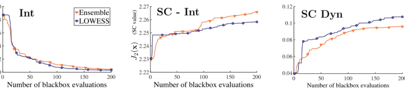
Figure 4presents the performance of the optimization approaches for the three 10-d problem
396
formulations. The initial value for J1is 8.7 cents. The initial value for J2and J3 are 2.23 and 0.04
397
(value of SC), respectively, as can be seen in Figure5.
398 399
On average, the LOWESS surrogate approach yields slightly better designs for J1(x, ϕ) and
400
better results for J3(x, ϕ). For Int (J1) the best objective function value obtained is 0.1 cents,
0 50 100 150 200
Number of blackbox evaluations
0 2 4 6 8 10 Ensemble LOWESS (cents) J1 (x ) Int 0 50 100 150 200
Number of blackbox evaluations
2.22 2.23 2.24 2.25 2.26 2.27 (SC value) J2 (x ) SC - Int 0 50 100 150 200
Number of blackbox evaluations 0.04 0.06 0.08 0.1 0.12 SC Dyn
FIG. 4. Evolution of the objective function values for the 3 10-d problem formulations; from left to right: Int, SC Int, and SC Dyn (color online)
and the best intonation improvement is 8.6 cents. This represents a 99% improvement. For SC
-402
Int (J2) the best objective function value obtained is 2.27 (value of SC), and the average spectral
403
centroid improvement is 0.04. This represents a 1.8% overall improvement ((2.27 – 2.23)/ 2.23)).
404
For SC Dyn (J3) the best objective function value obtained is 0.14 (value of SC), and the spectral
405
centroid difference improvement is 0.1. This optimal bore improves 35 times the J3 performance
406
of the initial bore (0.14/ 0.04). Yet, measurements on an expert trumpet player playing B[4 concert
407
pitch show a SC increase around 0.8 between a p and f f note for the 6 first harmonics, which is
408
more than 5 times superior to the simulated values of the optimum. These results are in accordance
409
with (Petiot and Gilbert, 2013). Even if the method optimizes the spectral centroid variation, the
410
model does not allow the prediction of realistic spectral centroid values. Non-linear propagation
411
in the bore should be taken into account.
412
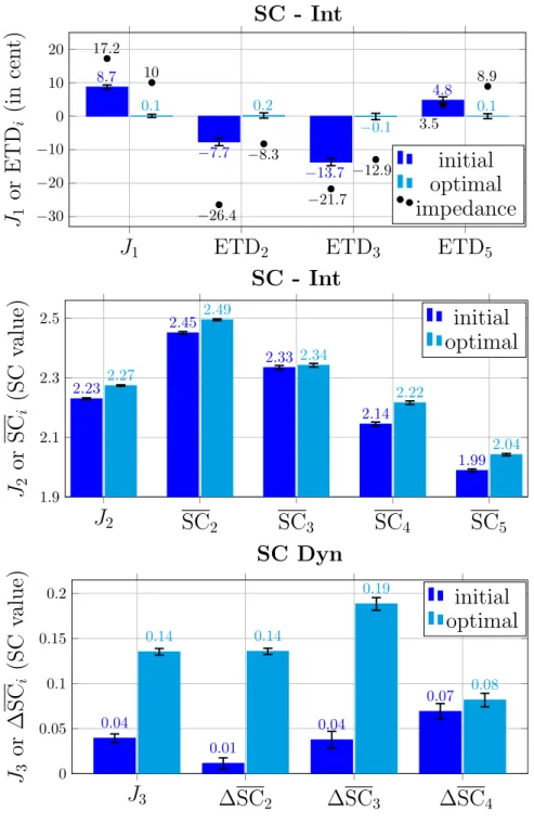
Figure5provides a finer acoustical analysis of these results showing the contributions of each
413
note to the objective functions for the initial bore and the optimal bore. The error bars are computed
414
following the guidelines of the Joint Committee for Guides in Metrology (JCGM,2008). For Int,
415
the B[3 and F4 show significant improvements of 7.5 and 13.6 cent, respectively, which are
J1
ETD2
ETD3
ETD5
−30 −20 −10 0 10 20 8.7 −7.7 −13.7 4.8 0.1 0.2 −0.1 0.1 17.2 −26.4 −21.7 3.5 10 −8.3 −12.9 8.9J
1or
ETD
i(i
n
ce
n
t)
initial
optimal
impedance
SC - Int
J2
SC2
SC3
SC4
SC5
1.9 2.1 2.3 2.5 2.23 2.45 2.33 2.14 1.99 2.27 2.49 2.34 2.22 2.04J
2or
S
C
i(S
C
va
lu
e)
SC - Int
initial
optimal
J
3∆SC
2∆SC
3∆SC
4 0 0.05 0.1 0.15 0.2 0.04 0.01 0.04 0.07 0.14 0.14 0.19 0.08J
3or
∆
S
C
i(S
C
va
lu
e)
SC Dyn
initial
optimal
FIG. 5. On the top part, the columns represent from left to right J1value and the non zero ETDs. Two bores are evaluated, the initial bore of all the optimization jobs and the best bore from the most successful job (out of the 20 available). The error bars equal to 2 standard deviations of the estimated quantity. Equivalent plots for the design problems SC - Int and SC Dyn are drawn below. SCiis SC restricted to ϕi. In addition, the values of J1and the corresponding ETDs, obtained with the input impedance peaks frequency values,
rior to the classical just-noticeable difference (JND) of 5 cents. B[4 being the relative reference, it
417
is always considered perfectly in tune. Since the initial value of D5 is already low (4.8 cent) the
418
improvement of 4.7 cent is slightly lower than the JND. The sound simulation results concerning
419
intonation are in agreement with the impedance peaks frequency values except for D5, for which
420
the optimal trumpet seems less in tune when considering the impedance peaks frequency values.
421
For SC - Int, the highest improvement is 0.08 (value of SC) for B[4 which is at the same level
422
than the JND of 0.1 reported in (Jeong and Fricke, 1998). Consequently, for B[3, F4 and D5, the
423
improvements seem negligible, rising to 0.04, 0.01 (error bars level), and 0.5, respectively. For SC
424
Dyn, the improvements for B[3 and F4 are above the JND (0.13 and 0.15, respectively), contrary
425
to B[4 (0.01).
426
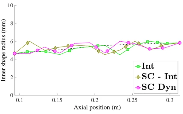
Figure6shows the leadpipes yielding the best value for each design problem.
427
As in (Tournemenne et al., 2017), the optima are counter intuitive since the leadpipe does
428
not have a positive slope along the whole trumpet axis. This kind of shape for a leadpipe is not
429
common among trumpets because it is very difficult to manufacture. The optimization algorithm
430
was able to explore the design space in order to find unusual designs. Finally, the geometrical
431
differences between the 3 optima and the initial leadpipe are on the order of the millimeter for
432
several control radii, which will lead to noticeably different instruments when manufactured.
433
B. Discussion
434
Concerning intonation, the objective function value based on sound simulations is always below
435
the one obtained only with the input impedance peaks (cf. black dots of Figure5). This has been
436
verified on more examples (Tournemenne,2017), and would mean that the musician always plays
0.1
0.15
0.2
0.25
0.3
Axial position (m)
0
2
4
6
8
10
Inner shape radius (mm)
Int
SC - Int
SC Dyn
FIG. 6. Representation of the leadpipe inner radius along the instrument axis; the black dotted line to the initial geometry (measured on our trumpet); each other line corresponds to the best design found by each objective over 20 jobs (color online)
more in tune that would suggest the resonance frequency values of the input impedance. This is
438
necessarily an effect of the non-linear part of the model which requires further study. The history
439
plot of the Int design problem demonstrates a significant intonation improvement, above JND:
440
the objective function is decreased by 99% to 0.1 cents. Such a level of performance has been
441
achieved for a small price (200 evaluations compared with the million evaluations needed by brute
442
force). Future studies may consider even more design variables. Concerning the spectral centroid,
443
the results show improvements of the objective function J2 and J3, even if they remain limited
444
and close to the JND. More marked improvements would certainly occur on real trumpets when
445
played.
Regarding the surrogate modeling approach, it is hard to tell whether one is consistently better
447
than the other as they seem to exhibit the same exploration to exploitation ratio of the design
448
space. It should be noted that the locally weighted regression models take longer to compute than
449
the ensemble of surrogates in high-dimensional problems (in our case, the difference is one hour
450
vs. few minutes for ten variables).
451
VI. CONCLUSIONS
452
In this paper, we extended a new paradigm for design optimization of brass instruments. This
453
new paradigm goes beyond impedance based optimization.(Braden et al.,2009;Guilloteau,2015;
454
Kausel, 2001; Macaluso and Dalmont, 2011;Noreland et al., 2013, 2010; Poirson et al., 2007).
455
We consider the optimization of objective functions (possibly subject to constraints) based directly
456
on the sounds spectrum, which, to the best of our knowledge, is a novel approach. The
original-457
ity of the approach lies in the fact that the objective function is not limited to a characterization
458
of the instrument alone, but includes virtual musicians in an physical model, to optimize directly
459
the instrument sounds. The main contribution of this paper is to demonstrate how physics-based
460
sound simulations can be integrated in an iterative optimization algorithm, which requires that
461
simulations converge automatically toward auto-oscillations for every considered bore of the
de-462
sign space, without any assistance of the user. A second contribution concerns the optimization
463
of objective functions based on a particular dimension of the timbre of the sounds, the spectral
464
centroid. Applied to the optimization of a trumpet, the results show that the optimization method,
465
based on the MADS algorithm, is efficient to define optimal solutions in a reasonable computation
466
time, with or without constraints, for problems up to 10 design variables.
While the approach shows promising potential, there is room for improvement. Even if it is
ef-468
ficient to reproduce differences between instruments concerning intonation and spectral centroid,
469
the elementary model could be improved to generate a more realistic sound spectrum. The sound
470
optimized in this work is the sound in the mouthpiece. Even if this does not change the principle
471
of the method presented, it could be interesting to define a relevant radiated pressure outside the
472
instrument, and to include it in the optimization considerations. Another valuable contribution to
473
this numerical study concerns the manufacturing of the optimal instruments and their objective
474
and subjective study. This would help evaluate actual improvement. Regarding implementation,
475
the influence of the selection process of the virtual embouchure could be investigated further, as it
476
may provide more robust descriptors of the ease of playing of the considered instruments.
Regard-477
ing the methodology, a study of temporal sound simulations could lead to new classes of objective
478
functions, such as attack times. More ambitious still, the inclusion of non-linear propagation in
479
simulations would produce more realistic sounds improving the objective functions considered
480
in this work. Finally, the main challenge in the design of musical instrument lies in the
defini-481
tion of judicious objective functions providing actual insight of the instrument intrinsic quality.
482
This task may be accomplished by working side-by-side with instrument makers whose empirical
483
understanding may be translated to computational principles and models.
484
ACKNOWLEDGMENTS
485
The authors are grateful to the NOMAD team (Prof. Charles Audet, Prof. S´ebastien Le Digabel
486
and Dr. Christophe Tribes), Prof. Sa¨ıd Moussaoui for his help with the optimization problem
487
formulation, Prof. Jean-Pierre Dalmont for his precious help with the input impedance models,
and Juliette Chabassier for the many helpful discussions. Numerical experiments were carried out
489
using the PlaFRIM experimental testbed (seehttps://www.plafrim.fr/).
490
1See Supplementary materials at [URL will be inserted by AIP] for the sounds.
491
492
Adachi, S., and Sato, M.-a. (1996). “Trumpet sound simulation using a two-dimensional lip
vibra-493
tion model,” The Journal of the Acoustical Society of America 99(2), 1200–1209.
494
Audet, C., and Dennis, Jr., J. E. (2006). “Mesh adaptive direct search algorithms for constrained
495
optimization,” SIAM Journal on Optimization 17(1), 188–217.
496
Audet, C., Kokkolaras, M., Le Digabel, S., and Talgorn, B. (2018). “Order-based error for
man-497
aging ensembles of surrogates in derivative-free optimization,” Journal of Global Optimization
498
70(3), 645–675.
499
Benade, A. H. (1966). “Relation of AirColumn resonances to sound spectra produced by wind
500
instruments,” J. Acoust. Soc. Am. 40(1), 247–249.
501
Boutin, H., Fletcher, N., Smith, J., and Wolfe, J. (2015). “Relationships between pressure, flow,
502
lip motion, and upstream and downstream impedances for the trombone,” The Journal of the
503
Acoustical Society of America 137(3), 1195–1209.
504
Braden, A. C. P., Newton, M. J., and Campbell, D. M. (2009). “Trombone bore optimization based
505
on input impedance targets,” J. Acoust. Soc. Am. 125(4), 2404–2412.
506
Bromage, S., Campbell, M., and Gilbert, J. (2010). “Open areas of vibrating lips in trombone
507
playing,” Acta Acustica united with Acustica 96(4), 603–613.
Campbell, M. (2004). “Brass instruments as we know them today,” Acta Acustica united with
509
Acustica 90(4), 600–610.
510
Causs´e, R., Kergomard, J., and Lurton, X. (1984). “Input impedance of brass musical
511
instruments—comparison between experiment and numerical models,” J. Acoust. Soc. Am.
512
75(1), 241–254.
513
Chen, F.-C., and Weinreich, G. (1996). “Nature of the lip reed,” The Journal of the Acoustical
514
Society of America 99(2), 1227–1233.
515
Cullen, J., Gilbert, J., and Campbell, M. (2000). “Brass instruments: Linear stability analysis and
516
experiments with an artificial mouth,” Acta Acustica united with Acustica 86(4), 704–724.
517
Deutsch, D. (2013). The Psychology of Music (Third Edition) (Academic Press).
518
Elliott, S., and Bowsher, J. (1982). “Regeneration in brass wind instruments,” Journal of Sound
519
and Vibration 83(2), 181–217.
520
Eveno, P., Petiot, J.-F., Gilbert, J., Kieffer, B., and Causs´e, R. (2014). “The relationship between
521
bore resonance frequencies and playing frequencies in trumpets,” Acta Acustica united with
522
Acustica 100(2), 362–374.
523
Fletcher, N. H., and Tarnopolsky, A. (1999). “Blowing pressure, power, and spectrum in trumpet
524
playing,” J. Acoust. Soc. Am. 105(2), 874–881.
525
Gilbert, J., Kergomard, J., and Ngoya, E. (1989). “Calculation of the steady-state oscillations of a
526
clarinet using the harmonic balance technique,” J. Acoust. Soc. Am. 86(1), 35–41.
527
Guilloteau, A. (2015). “Conception d’une clarinette logique” (“Design of a logical clarinet”),
528
Ph.D. thesis, Aix-Marseille.
Jeong, D., and Fricke, F. R. (1998). “The dependence of timbre perception on the acoustics of
530
the listening environment,” in Proc. 16th Int. Congress on Acoustics and 135th Meeting of the
531
Acoustical Society of America, Vol. 3, pp. 2225–2226.
532
JCGM (2008). “Evaluation of measurement data – guide to the expression of uncertainty in
mea-533
surement,” Technical Report .
534
Kausel, W. (2001). “Optimization of brasswind instruments and its application in bore
reconstruc-535
tion,” Journal of New Music Research 30(1), 69–82.
536
Le Digabel, S. (2011). “Algorithm 909: NOMAD: Nonlinear optimization with the MADS
algo-537
rithm,” ACM Trans. Math. Softw. 37(4), 44:1–44:15.
538
Macaluso, C. A., and Dalmont, J.-P. (2011). “Trumpet with near-perfect harmonicity: design and
539
acoustic results,” J. Acoust. Soc. Am. 129(1), 404–414.
540
Martin, D. W. (1942). “Directivity and the acoustic spectra of brass wind instruments,” The Journal
541
of the Acoustical Society of America 13(3), 309–313.
542
Myers, A., Pyle Jr, R. W., Gilbert, J., Campbell, D. M., Chick, J. P., and Logie, S. (2012). “Effects
543
of nonlinear sound propagation on the characteristic timbres of brass instruments,” The Journal
544
of the Acoustical Society of America 131(1), 678–688.
545
Newton, M. J., Campbell, M., and Gilbert, J. (2008). “Mechanical response measurements of real
546
and artificial brass players lips,” J. Acoust. Soc. Am. 123(1), EL14–20.
547
Noreland, D., Kergomard, J., Lalo¨e, F., Vergez, C., Guillemain, P., and Guilloteau, A. (2013).
548
“The logical clarinet: Numerical optimization of the geometry of woodwind instruments,” Acta
549
Acustica united with Acustica 99(4), 615–628.
Noreland, J. O. D., Udawalpola, M. R., and Berggren, O. M. (2010). “A hybrid scheme for bore
551
design optimization of a brass instrument,” J. Acoust. Soc. Am. 128(3), 1391–1400.
552
Petiot, J.-F., and Gilbert, J. (2013). “Comparison of trumpets’ sounds played by a musician or
553
simulated by physical modelling,” Acta Acustica united with Acustica 98, 475–486.
554
Poirson, E., Petiot, J.-F., and Gilbert, J. (2005). “Study of the brightness of trumpet tones,” The
555
Journal of the Acoustical Society of America 118(4), 2656–2666.
556
Poirson, E., Petiot, J.-F., and Gilbert, J. (2007). “Integration of user perceptions in the design
pro-557
cess: Application to musical instrument optimization,” Journal of Mechanical Design 129(12),
558
1206–1214.
559
Talgorn, B., Audet, C., Le Digabel, S., and Kokkolaras, M. (2018). “Locally weighted regression
560
models for surrogate-assisted design optimization,” Optimization and Engineering 19(1), 213–
561
238.
562
Tournemenne, R. (2017). “Optimisation d’un instrument de musique de type cuivre bas´ee sur des
563
simulations sonores par mod`ele physique” (“Brass instrument optimization based on
physics-564
based sound simulations”), Ph.D. thesis, ´Ecole Centrale de Nantes.
565
Tournemenne, R., Petiot, J.-F., Talgorn, B., Kokkolaras, M., and Gilbert, J. (2017). “Brass
instru-566
ments design using physics-based sound simulation models and surrogate-assisted
derivative-567
free optimization,” Journal of Mechanical Design 139(4), 041401.
568
Velut, L., Vergez, C., Gilbert, J., and Djahanbani, M. (2017). “How well can linear stability
analy-569
sis predict the behaviour of an Outward-Striking valve brass instrument model?,” Acta Acustica
570
united with Acustica 103(1), 132–148.
Yoshikawa, S. (1995). “Acoustical behavior of brass player’s lips,” the Journal of the Acoustical
572
Society of America 97(3), 1929–1939.