Characterization of Some Aggregation Functions Stable for
Positive Linear Transformations
Jean-Luc Marichal∗ Pierre Mathonet† Eric Tousset†
Revised version, February 28, 1997
Abstract
This paper deals with the characterization of some classes of aggregation functions often used in multicriteria decision making problems. The common properties involved in these characterizations are “increasing monotonicity” and “stability for positive linear transforma-tions”. Additional algebraic properties related to associativity allow to completely specify the functions.
Keywords: aggregation functions; interval scale; invariance; algebraic properties of aggregation functions; fuzzy multiple criteria decision making.
1
Introduction
Synthesizing judgments is an important part of multiple criteria decision making methods. The most typical situation concerns individuals who form quantifiable judgments about a measure of an object (weight, length, area, height, volume, importance or other attributes, for instance in the framework of a hierarchy)(see [3, 4]) or quantifiable judgments on pairs of alternatives along each criterion. In the latter case, the judgments are very often expressed with the help of fuzzy preference relations (see [8, 9]).
In order to reach a consensus (overall opinion) on these jugdments, classical aggregation func-tions have been proposed: arithmetic means, geometric means, root-power means and many others. Of course, given such an aggregation function, we can ask for a motivation of its use, i.e. for natural, reasonable assumptions which lead to this function. Conversely, we can specify some assumptions (called axioms or properties) and determine all the aggregation functions satisfying these. This is the topic with which we deal here.
This paper aims at describing the family of all aggregation functions fulfilling three specific properties. The first two are increasing monotonicity and stability for the same transformations of interval scales in the sense of the theory of measurement (see [15]), i.e. stability for positive linear transformations (we refer to the corresponding functional equation in [5, 6] where the arithmetic mean is characterized). The third property is chosen among well-known algebraic properties such as associativity, decomposability and bisymmetry. See Section 3 for details.
We make a distinction between aggregation functions having a fixed number of arguments and aggregation functions defined for all number of arguments (aggregators). Section 4 is devoted to characterizations of aggregation functions with a fixed number of arguments whereas Section 5 presents characterizations of aggregators.
∗Ecole d’Administration des Affaires, Universit´e de Li`ege, Boulevard du Rectorat 7 - B31, B-4000 Li`ege, Belgium.
Email: jl.marichal[at]ulg.ac.be
2
Basic definitions
We first want to define the concept of aggregation function. In this paper, IN∗ denotes the set of strictly positive integers and IR the set of real numbers. Moreover, we assume that the information to be aggregated consists of numbers belonging to the interval [0, 1] as required in most applications. In Section 7, we show that this assumption can be weakened.
Definition 2.1 Let m ∈ IN∗. An aggregation function M(m) defined on [0, 1]m is a real valued function of m arguments:
M(m): [0, 1]m → IR : (x1, . . . , xm) → M(m)(x1, . . . , xm). For instance, the arithmetic mean function defined by
AM(m)(x1, . . . , xm) = 1 m m X i=1 xi ∀(x1, . . . , xm) ∈ [0, 1]m is an aggregation function defined on [0, 1]m.
Definition 2.2 An aggregator M defined on Sm≥1[0, 1]m is a sequence (M(m))
m∈IN∗ whose mth
element is an aggregation function M(m) defined on [0, 1]m: M : [
m≥1
[0, 1]m→ IR : (x1, . . . , xm) → M(m)(x1, . . . , xm). For instance, the arithmetic mean aggregator is AM = (AM(m))
m∈IN∗.
Let m ∈ IN∗. We consider a discrete set of m elements Nm = {1, . . . , m}, which could be players of a cooperative game, criteria, attributes or voters in a decision making problem.
In order to avoid heavy notations, we introduce the following terminology. It will be used all along this paper.
• II := [0, 1]
• For all k ∈ IN∗ and all x ∈ II, k · x := x, . . . , x | {z }
k
• For all N ⊆ Nm, the characteristic vector of N in {0, 1}m is defined by e(m)N := (x1, . . . , xm) ∈ {0, 1}m with xi = 1 ⇔ i ∈ N.
Of course, the e(m)N ’s (N ⊆ Nm) are the 2m vertices of the hypercube IIm. We also introduce the complementary characteristic vector of N ⊆ Nm:
e(m)N := e(m)Nm\N. Then we set
θ(m)N := M(m)(e(m)N ) and θ(m)N := M(m)(e(m)N ).
The expressions e(m){i}, e(m){i}, θ(m){i}, θ(m){i} will be denoted e(m)i , e(m)i , θi(m), θ(m)i respectively. • Given a vector (x1, . . . , xm) ∈ IIm, let x
(1), . . . , x(m)denote the elements of this vector sorted
3
Aggregation properties
As mentioned in the introduction, if we want to obtain a reasonable or satisfactory aggregation, any aggregation function should not be used. In order to evacuate the “undesirable” functions, we can adopt an axiomatic approach and impose that these functions fulfil some selected properties. Such properties can be divided into three categories: natural properties, stability properties and algebraic properties.
3.1 Natural properties
Definition 3.1 The aggregation function M(m) defined on IIm is
• symmetric (Sy) if M(m) is a symmetric function on IIm, i.e. if, for all permutations σ of Nm and all (x1, . . . , xm) ∈ IIm, we have
M(m)(x1, . . . , xm) = M(m)(xσ(1). . . , xσ(m)).
• increasing (In) if M(m) is increasing in each argument, i.e. if, for all i ∈ Nm and all x1, . . . , xm, x0i ∈ II, we have
xi < x0i ⇒ M(m)(x1, . . . , xi, . . . , xm) ≤ M(m)(x1, . . . , x0i, . . . , xm). • compensative (Comp) if, for all (x1, . . . , xm) ∈ IIm,
min(x1, . . . , xm) ≤ M(m)(x1, . . . , xm) ≤ max(x1, . . . , xm). • idempotent (I) if, for all x ∈ II,
M(m)(m · x) = x.
It should be noted that any compensative aggregation function defined on IIm necessarily takes its values in II. Moreover, we have the following result which can easily be checked:
Proposition 3.1 For every aggregation function M(m) defined on IIm, (i) (Comp) ⇒ (I)
(ii) (In, I) ⇒ (Comp)
The properties mentioned in Definition 3.1 can be adapted to aggregators as follows.
Definition 3.2 The aggregator M defined on Sm≥1IIm fulfils (Sy) (resp. (In), (Comp), (I)) if, for all m ∈ IN∗, mth aggregation function M(m) fulfils (Sy) (resp. (In), (Comp), (I)).
3.2 Stability properties
Definition 3.3 The aggregation function M(m) defined on IIm is • stable for the admissible similarities (SSI) if
M(m)(rx1, . . . , rxm) = rM(m)(x1, . . . , xm) for all (x1, . . . , xm) ∈ IIm and all r > 0 such that rx
i ∈ II for all i ∈ Nm. • stable for the admissible translations (STR) if
• stable for the admissible positive linear transformations (SPL) if
M(m)(rx1+ t, . . . , rxm+ t) = rM(m)(x1, . . . , xm) + t
for all (x1, . . . , xm) ∈ IIm and all r > 0, t ∈ IR such that rxi+ t ∈ II for all i ∈ Nm. • stable for the standard negation N (SSN) if
M(m)(1 − x1, . . . , 1 − xm) = 1 − M(m)(x1, . . . , xm) for all (x1, . . . , xm) ∈ IIm.
The use of stability properties supposes that the values to be aggregated are given according to some scale type as defined by Roberts [15]. Note that some characterization theorems were obtained by Nagumo [14] for (SSI) and (STR) and by Silvert [16] for (SSN) (see also [9, pp.117-126] and [13]). The next result gives some relations between stability properties. These relations will be useful in the sequel.
Proposition 3.2 For all aggregation function M(m) defined on IIm, we have (i) (SSI, STR) ⇔ (SPL)
(ii) (SSI) ⇒ M(m)(m · 0) = 0
(iii) (SPL) ⇒ (I)
(iv) (SSI, SSN) ⇒ (SPL) Proof. (i) Trivial.
(ii) It suffices to consider (x1, . . . , xm) = (m · 0). (iii) It suffices to use (i) and (ii).
(iv) By (i), it suffices to show that M(m)fulfils (STR). Let (x1, . . . , xm) ∈ IImand t ∈ [−1, 1] such that xi+ t ∈ II ∀i ∈ Nm. Let us prove that
M(m)(x1+ t, . . . , xm+ t) = M(m)(x1, . . . , xm) + t.
By (ii) and (SSN) we have M(m)(m · 1) = 1 − M(m)(m · 0) = 1. So we can assume that t lies in
the open interval (−1, 1). For all i ∈ Nm set yi = xi
1−t. We then have yi ∈ II ∀i ∈ Nm and
M(m)(x1, . . . , xm) (SSI)= (1 − t)M(m)(y1, . . . , ym) (SSN ) = (1 − t) − (1 − t)M(m)(1 − y1, . . . , 1 − ym) (SSI) = (1 − t) − M(m)[(1 − t) − x1, . . . , (1 − t) − xm] (SSN ) = −t + M(m)(x1+ t, . . . , xm+ t).
It clearly turns out, by the previous proposition, that the condition “r > 0” in the statement of (SSI) or (SPL) can be replaced by “r ≥ 0” without any effect.
The next proposition characterizes the aggregation functions M(m) defined on IIm and satis-fying (SPL). A similar characterization was obtained by Acz´el and Roberts [5, p.220 (Case 5b)] in the case of aggregation functions M(m) defined on IRm.
Proposition 3.3 An aggregation function M(m) defined on IIm fulfils (SPL) if and only if there exists an aggregation function F(m) defined on IIm such that, for all (x1, . . . , xm) ∈ IIm, we have
M(m)(x1, . . . , xm) = ( x if (x1, . . . , xm) = (x, . . . , x), (x(m)− x(1))F(m)h x1−x(1) x(m)−x(1), . . . , xm−x(1) x(m)−x(1) i + x(1) otherwise.
Proof. (Sufficiency). Trivial.
(Necessity). It suffices to consider F(m)= M(m).
Definition 3.4 The aggregator M defined onSm≥1IIm fulfils (SSI) (resp. (STR), (SPL), (SSN)) if, for all m ∈ IN∗, the mth aggregation function M(m) fulfils (SSI) (resp. (STR), (SPL), (SSN)).
This paper mostly concentrates on the characterization of aggregation functions and aggregators satisfying properties (In) and (SPL), as well as some additional properties such as (Sy), (SSN), or algebraic properties to be introduced next.
3.3 Algebraic properties
Definition 3.5 The aggregation function M(m) defined on IIm is • associative (A) if m = 2 and
M(2)(M(2)(x1, x2), x3) = M(2)(x1, M(2)(x2, x3))
for all (x1, x2, x3) ∈ II3.
• autodistributive (AD) if m = 2 and
M(2)(x1, M(2)(x2, x3)) = M(2)(M(2)(x1, x2), M(2)(x1, x3)), M(2)(M(2)(x1, x2), x3) = M(2)(M(2)(x1, x3), M(2)(x2, x3)) for all (x1, x2, x3) ∈ II3. • bisymmetric (B) if m ≥ 2 and M(m)(M(m)(x11, . . . , x1m), . . . , M(m)(xm1, . . . , xmm)) = M(m)(M(m)(x11, . . . , xm1), . . . , M(m)(x1m, . . . , xmm)) for all square matrices
X = x11 · · · x1m .. . ... xm1 · · · xmm ∈ IIm×m.
Note that those definitions make sense only if M(m) takes its values in II.
The properties mentioned in Definition 3.5 were investigated by several authors. For a list of references see [2]. Ling [11] has specifically investigated the associative property (A). Bisymmetry (B) has been used by Acz´el [1] and Fodor and Marichal [7] to characterize certain mean values. This property expresses that aggregation can be performed first on the rows, then on the columns of any square matrix, or conversely. The next proposition presents an immediate link between (B) and (AD).
Proposition 3.4 For every aggregation function M(2) defined on II2, we have (I, B)⇒(AD).
The next algebraic properties concern aggregators.
• associative (A) if each subset of consecutive elements from (x1, . . . , xm) can be substituted by the partial aggregation of this subset without changing the global aggregation, i.e. formally, if M(1)(x) = x ∀x ∈ II and if, for all m ∈ IN∗, all (x
1, . . . , xm) ∈ IIm and all 0 ≤ j < k ≤ m, we have
M(m)(x1, . . . , xj, xj+1, . . . , xk, xk+1, . . . , xm)
= M(m−k+j+1)(x1, . . . , xj, M(k−j)(xj+1, . . . , xk), xk+1, . . . , xm).
• decomposable (D) if each element of any subset of consecutive elements from (x1, . . . , xm) can be substituted by the partial aggregation of this subset without changing the global aggre-gation, i.e. formally, if M(1)(x) = x ∀x ∈ II and if, for all m ∈ IN∗, all (x1, . . . , xm) ∈ IIm and all 0 ≤ j < k ≤ m, we have
M(m)(x1, . . . , xj, xj+1, . . . , xk, xk+1, . . . , xm)
= M(m)(x1, . . . , xj, (k − j) · M(k−j)(xj+1, . . . , xk), xk+1, . . . , xm).
• strongly decomposable (SD) if each element of any subset of elements from (x1, . . . , xm) can be substituted by the partial aggregation of this subset without changing the global aggregation, i.e. formally, if M(1)(x) = x ∀x ∈ II and if, for all m ∈ IN∗, all (x
1, . . . , xm) ∈ IIm and all N = {i1, . . . , ip} ⊆ Nm, with i1 < . . . < ip, we have
M(m)(x1, . . . , xm) = M(m)(x01, . . . , x0m) where, for all i ∈ Nm,
x0i = (
xi if i 6∈ N,
M(p)(xi1, . . . , xip) otherwise.
• strongly bisymmetric (SB) if M(1)(x) = x ∀x ∈ II and if, for all m, p ∈ IN∗, M(p)(M(m)(x11, . . . , x1m), . . . , M(m)(xp1, . . . , xpm)) = M(m)(M(p)(x11, . . . , xp1), . . . , M(p)(x1m, . . . , xpm)) for all matrices
X = x11 · · · x1m .. . ... xp1 · · · xpm ∈ IIp×m.
Note that those definitions make sense only if, for all m ∈ IN∗, M(m) takes its values in II.
Associativity (A) is a well-known algebraic property which allows to omit “parentheses” in an ag-gregation of at least three elements (see e.g. [2]). Observe that, if the aggregator M is associative, then the function M(2) is associative (just set m = 3 in Definition 3.6). Of course, associativity
can be viewed as an iterative property since it allows to define completely any aggregator M only from its function M(2).
Decomposability is a property introduced by Kolmogoroff [10] and Nagumo [14] in the case of symmetric aggregators (Sy)(see also [7]). In the nonsymmetric case, we generalize this property in two ways: decomposability (D) and strong decomposability (SD). Of course, under (Sy), these two properties are identical. We also introduce the property of strong bisymmetry (SB) as a generalization of (B).
Proposition 3.5 For every aggregator M defined on Sm≥1IIm, we have (I, A)⇒(D). Proof. Let m ∈ IN∗ and (x
1, . . . , xm) ∈ IIm. We have, if 0 ≤ j < k ≤ m, M(m)(x1, . . . , xj, xj+1, . . . , xk, xk+1, . . . , xm) (A) = M(m−k+j+1)(x1, . . . , xj, M(k−j)(xj+1, . . . , xk), xk+1, . . . , xm) (I) = M(m−k+j+1)(x1, . . . , xj, M(k−j)((k − j) · M(k−j)(xj+1, . . . , xk)), xk+1, . . . , xm) (A) = M(m)(x1, . . . , xj, (k − j) · M(k−j)(xj+1, . . . , xk), xk+1, . . . , xm).
4
Characterization of some aggregation functions
This section is devoted to aggregation functions M(m) which are increasing and stable for positive linear transformations. The next definition introduces some of them (all are defined on IIm). Definition 4.1 Let m ∈ IN∗.
• For any weight vector ω(m)= (ω1(m), . . . , ωm(m)) ∈ IIm such that m
X i=1
ωi(m)= 1,
the weighted arithmetic mean function WAM(m)ω(m) and the ordered weighted averaging
func-tion OWA(m)ω(m) associated to ω(m), are respectively defined by
WAM(m)ω(m)(x1, . . . , xm) = m X i=1 ωi(m)xi ∀(x1, . . . , xm) ∈ IIm, OWA(m)ω(m)(x1, . . . , xm) = m X i=1 ωi(m)x(i) ∀(x1, . . . , xm) ∈ IIm.
• The arithmetic mean function AM(m) is defined by
AM(m)(x1, . . . , xm) = m1 m X i=1
xi ∀(x1, . . . , xm) ∈ IIm.
• For any i ∈ Nm, the projection function P(m)i associated to the ith argument is defined by P(m)i (x1, . . . , xm) = xi ∀(x1, . . . , xm) ∈ IIm.
• The minimum function MIN(m) and the maximum function MAX(m)are respectively defined
by MIN(m)(x1, . . . , xm) = min i∈Nm xi ∀(x1, . . . , xm) ∈ IIm, MAX(m)(x1, . . . , xm) = max i∈Nm xi ∀(x1, . . . , xm) ∈ IIm.
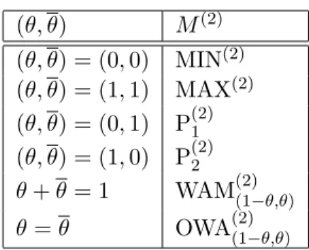
(θ, θ) M(2) (θ, θ) = (0, 0) MIN(2) (θ, θ) = (1, 1) MAX(2) (θ, θ) = (0, 1) P(2)1 (θ, θ) = (1, 0) P(2)2 θ + θ = 1 WAM(2)(1−θ,θ) θ = θ OWA(2)(1−θ,θ)
Table 1: Some examples • For any nonempty subset N(m) ⊆ N
m, the partial minimum function MIN(m)N(m) and the
partial maximum function MAX(m)N(m) associated to N(m), are respectively defined by
MIN(m)N(m)(x1, . . . , xm) = min i∈N(m)xi ∀(x1, . . . , xm) ∈ II m, MAX(m)N(m)(x1, . . . , xm) = max i∈N(m)xi ∀(x1, . . . , xm) ∈ II m.
The following result shows that any aggregation function M(2) defined on II2 and fulfilling (In,
SPL) is completely defined by the values M(2)(0, 1) and M(2)(1, 0).
Proposition 4.1 The aggregation function M(2) defined on II2 fulfils (In, SPL) if and only if, for
all (x1, x2) ∈ II2, we have M(2)(x1, x2) = ( (1 − θ)x1+ θx2 if x1 ≤ x2, θx1+ (1 − θ)x2 if x1 ≥ x2, = θx1+ θx2+ (1 − θ − θ)(x1∧ x2),
with θ, θ ∈ II. Moreover, we have θ = M(2)(0, 1) and θ = M(2)(1, 0). Proof. (Sufficiency). Easy.
(Necessity). Let (x1, x2) ∈ II2. If x1 ≤ x2 then we have
M(2)(x1, x2)(SP L)= (x2− x1)M(2)(0, 1) + x1 = (1 − θ)x1+ θx2
with θ = M(2)(0, 1). Moreover, θ ∈ II since, by Propositions 3.1 and 3.2, M(2) is compensative.
One proceeds similarly if x1≥ x2.
Some particular examples according to the values of θ and θ can be found in Table 1. Moreover, the next corollary trivially follows.
Corollary 4.1 The aggregation function M(2) defined on II2 fulfils (Sy, In, SPL) if and only if
there exists ω(2)∈ II2 such that
M(2) = OWA(2)ω(2).
Note that a complete characterization of the OWA(m)ω(m) functions can be found in [12] (see also [9,
p.133]).
The next two theorems describe the families of aggregation functions M(2) defined on II2 and
fulfilling (In, SPL, A), (In, SPL, AD) and (In, SPL, B) respectively.
Theorem 4.1 The aggregation function M(2) defined on II2 fulfils (In, SPL, A) if and only if M(2) ∈ {MIN(2), MAX(2), P(2)
Proof. (Sufficiency). Trivial.
(Necessity). Set θ = M(2)(0, 1) and θ = M(2)(1, 0). By Proposition 4.1, we only have to prove
that θ, θ ∈ {0, 1}. The aggregation function M(2) must fulfil the equation
M(2)(M(2)(x1, x2), x3) = M(2)(x1, M(2)(x2, x3))
for all (x1, x2, x3) ∈ II3. In particular, for (x1, x2, x3) = e(3)3 , we obtain, by (SSI), θ ∈ {0, 1}. Also,
for (x1, x2, x3) = e(3)1 , we obtain θ ∈ {0, 1}.
Theorem 4.2 Let M(2) be any aggregation function defined on II2. Then the following three
assertions are equivalent:
(i) M(2) fulfils (In, SPL, AD),
(ii) M(2) fulfils (In, SPL, B),
(iii) M(2) ∈ {MIN(2), MAX(2)} ∪ {WAM(2)ω(2)|ω(2)∈ II2}.
Proof. (iii) ⇒ (ii). Trivial.
(ii) ⇒ (i). It is a straightforward consequence of Propositions 3.2 and 3.4.
(i) ⇒ (iii). Set θ = M(2)(0, 1) and θ = M(2)(1, 0). By Proposition 4.1, we only have to prove
that (θ, θ) ∈ {(0, 0), (1, 1)} or θ + θ = 1. The aggregation function M(2) must fulfil the equation
M(2)(x1, M(2)(x2, x3)) = M(2)(M(2)(x1, x2), M(2)(x1, x3))
for all (x1, x2, x3) ∈ II3. In particular, for (x1, x2, x3) = (θ, 0, 1), we obtain, by Proposition 4.1,
θ = M(2)(θθ, θ(2 − θ)) = (1 − θ)θθ + θ2(2 − θ)
and so, θ = 0 or θ = 1 or θ + θ = 1. Similarly, for (x1, x2, x3) = (θ, 1, 0), we obtain, by Proposition
4.1,
θ = M(2)((1 − θ)θ + θ, θ2) = θ2(1 − θ) + θθ + (1 − θ)θ2 and so, θ = 0 or θ = 1 or θ + θ = 1.
Corollary 4.2 Let M(2) be any aggregation function defined on II2. Then the following three
assertions are equivalent:
(i) M(2) fulfils (Sy, In, SPL, AD),
(ii) M(2) fulfils (Sy, In, SPL, B),
(iii) M(2) ∈ {MIN(2), MAX(2), AM(2)}.
Before obtaining the description of the family of functions M(m) defined on IIm (m ≥ 2) and fulfilling (In, SPL, B), we need three technical lemmas.
Lemma 4.1 Let m ∈ IN∗, m ≥ 2. If the aggregation function M(m) defined on IIm fulfils (In, SPL, B) and if there exists N ⊆ Nm such that θN(m)∈ (0, 1) then M(m) is additive, i.e.
M(m)(u1+ v1, . . . , um+ vm) = M(m)(u1, . . . , um) + M(m)(v1, . . . , vm) for all (u1, . . . , um), (v1, . . . , vm) ∈ IIm with u
Proof. Let (u1, . . . , um), (v1, . . . , vm) ∈ IIm with ui+ vi ∈ II ∀i ∈ Nm and set α = inf{θ(m)N , 1 − θ(m)N } ∈ (0, 1).
(i) Assume first that ui, vi ≤ α ∀i ∈ Nm. Consider the square matrix X of m rows ri and m columns cj (i, j ∈ Nm), where ri is defined as follows (for i ∈ Nm):
ri = 1 2 Ã ui θ(m)N + 1 ! e(m)N +1 2 vi 1 − θ(m)N e (m) N . On the one hand, by (SPL), we have, for all i ∈ Nm:
M(m)(ri) = 12 vi 1 − θN(m) + 1 2 Ã ui θ(m)N + 1 − vi 1 − θ(m)N ! θN(m)= ui+ vi 2 + θ(m)N 2 , and thus M(m)(M(m)(r1), . . . , M(m)(rm)) = 21M(m)(u1+ v1, . . . , um+ vm) + θ (m) N 2 . On the other hand, for all j ∈ Nm, we have
M(m)(cj) = 1 2 µ M(m)(u 1,...,um) θN(m) + 1 ¶ if j ∈ N, 1 2 M(m)(v 1,...,vm) 1−θ(m)N otherwise.
However, by Propositions 3.1 and 3.2, M(m) fulfils (Comp). Hence, by (SPL), we have,
M(m)(M(m)(c1), . . . , M(m)(cm)) = M(m) " 1 2 Ã M(m)(u 1, . . . , um) θN(m) + 1 ! e(m)N +1 2 M(m)(v 1, . . . , vm) 1 − θN(m) e (m) N # = 1 2 h M(m)(u1, . . . , um) + M(m)(v1, . . . , vm)i+θ (m) N 2 . Since M(m) fulfils (B), we have
M(m)(u1+ v1, . . . , um+ vm) = M(m)(u1, . . . , um) + M(m)(v1, . . . , vm). (ii) In the general case, we have,
M(m)(u1+ v1, . . . , um+ vm) (SP L)= 1 αM (m)(αu 1+ αv1, . . . , αum+ αvm) (i) = 1 αM (m)(αu 1, . . . , αum) +α1M(m)(αv1, . . . , αvm) (SP L) = M(m)(u1, . . . , um) + M(m)(v1, . . . , vm).
Lemma 4.2 Let m ∈ IN∗, m ≥ 2. If the aggregation function M(m) defined on IIm fulfils (In, SPL, B), and if θN(m) ∈ {0, 1} ∀N ⊆ Nm, then, setting Nmax = {i ∈ Nm|θ(m)i = 1} and assuming Nmax6= ∅, we have, for all N ⊆ Nm:
Proof. The result is trivial if m = 2. Otherwise, use induction on |N |.
The result holds for |N | ∈ {0, 1}. Assume that it holds for |N | = n ≥ 1 and show that it holds for |N | = n + 1. Assume that N ∩ Nmax= ∅ and consider the square matrix X of m rows ri and m columns cj (i, j ∈ Nm), where ri is defined as follows (for i ∈ Nm):
ri = (m · 0) if i 6∈ N e(m)N if i = q (m · 1) if i ∈ N \ {q} where q ∈ N . On the one hand, for all i ∈ N \ {q}, we have M(m)(r
i) = 1. On the other hand, for all j ∈ Nm, we have
M(m)(cj) = (
0 if j 6∈ N (by induction), θ(m)N if j ∈ N.
Indeed, if j 6∈ N , we have cj = e(m)N \{q}and (N \ {q}) ∩ Nmax= ∅.
Now, let j0∈ N \ {q}. In particular, we have j0 6∈ Nmax. Consider the square matrix X0 of m rows r0i and m columns c0j (i, j ∈ Nm), where r0i= ri for all i ∈ Nm\ {j0} and r0j0 = e
(m)
j0 . We then
have
M(m)(e(m)j0 ) = θ(m)j0 = 1 since, by (In), θ(m)j0 ≥ θ(m)i for all i ∈ Nmax. So we have
M(m)(M(m)(r01), . . . , M(m)(rm0 )) = M(m)(M(m)(r1), . . . , M(m)(rm)). However, since c0 j0 = e (m) N \{j0}, we have M (m)(c0
j0) = 0 (by induction) and
M(m)(c0j) = 0 if j 6∈ N, 0 if j = j0, θ(m)N if j ∈ N \ {j0}.
Consequently, since M(m) fulfils (SPL) and (B), we have
[θN(m)]2 = M(m)(M(m)(c1), . . . , M(m)(cm)) = M(m)(M(m)(r1), . . . , M(m)(rm)) = M(m)(M(m)(r01), . . . , M(m)(r0m)) = M(m)(M(m)(c01), . . . , M(m)(c0m)) = θN(m) M(m)(e(m)N \{j
0}) = 0.
Lemma 4.3 Let m ∈ IN∗, m ≥ 2. If the aggregation function M(m)defined on IIm fulfils (In, SPL, B), if θN(m) ∈ {0, 1} ∀N ⊆ Nm and θi(m) = 0 ∀i ∈ Nm, then, setting Nmin = {i ∈ Nm|θ(m)i = 0}, we have Nmin 6= ∅ and θ(m)Nmin = 1.
Proof. If m = 2 then θ(2)1 = θ(2)2 = 0 and θ(2)2 = θ(2)1 = 0. Otherwise, let N∗
min ⊆ Nm with a minimal cardinality such that θ(m)N∗
min = 1. The existence of such a N
∗
minis trivial since θ(m)Nm = 1, and
we clearly have |N∗
min| ≥ 2. Let us prove that Nmin∗ ⊆ Nmin. Assume that there exists k ∈ Nmin∗
such that θ(m)k = 1. Consider the square matrix X of m rows ri and m columns cj (i, j ∈ Nm), where ri is defined as follows (for i ∈ Nm):
ri= (m · 0) if i 6∈ N∗ min e(m)N∗ min if i = k
On the one hand, we have, for all i ∈ Nm: M(m)(ri) = ( 0 if i 6∈ N∗ min 1 if i ∈ N∗ min and thus M(m)(M(m)(r1), . . . , M(m)(rm)) = M(m)(e(m)N∗ min) = θ (m) N∗ min = 1.
On the other hand, for all j ∈ Nm, we have
M(m)(cj) = 0 if j 6∈ N∗
min since |Nmin∗ | is minimal,
0 if j = k since θ(m)i = 0 ∀i ∈ Nm, 1 if j ∈ N∗
min\ {k} since cj = e(m)N∗ min.
Since M(m) fulfils (B), we have
1 = M(m)(M(m)(c1), . . . , M(m)(cm)) = M(m)(e(m)N∗ min\{k}),
a contradiction since |N∗
min| is minimal.
Now, let us prove that Nmin ⊆ N∗
min. For all i 6∈ Nmin∗ , we have, by (In), θ (m)
i ≥ θN(m)∗ min = 1,
that is i 6∈ Nmin.
Theorem 4.3 Let m ∈ IN∗, m ≥ 2. The aggregation function M(m) defined on IIm fulfils (In, SPL, B) if and only if M(m)∈ {MIN(m)N(m), MAX (m) N(m)|N(m)⊆ Nm} ∪ {WAM (m) ω(m)|ω(m)∈ IIm}.
Proof. (Sufficiency). Trivial.
(Necessity). Let (x1, . . . , xm) ∈ IIm. The values θ(m)
N (N ⊆ Nm) fulfil the assumptions of exactly one of Lemmas 4.1, 4.2 or 4.3. We then have three exclusive cases:
(i) Under the assumptions of Lemma 4.1, we have, by (SPL), M(m)(x1, . . . , xm) = m X i=1 θi(m)xi, with, by (I),Piθ(m)i = M(m)(m · 1) = 1.
(ii) Under the assumptions of Lemma 4.2, there exists p ∈ Nmax such that xp = maxi∈Nmaxxi
and we have
M(m)(x1, . . . , xm)
(In)
≤ M(m)(xp e(m)Nmax+ e(m)Nmax)(SP L)= xp+ (1 − xp)θ(m)Nmax = xp
and M(m)(x1, . . . , xm) (In) ≥ M(m)(xp e(m)p ) (SP L) = xp θ(m)p = xp. Therefore, we have M(m)(x1, . . . , xm) = max i∈Nmax xi.
(iii) Under the assumptions of Lemma 4.3, there exists p ∈ Nmin such that xp = mini∈Nminxi
and we have, since p ∈ Nmin:
M(m)(x1, . . . , xm)
(In)
≤ M(m)(xp e(m)p + e(m)p )
(SP L)
In, SPL, A (m = 2) Sy, In, SPL, A (m = 2) In, SSI, SSN, A (m = 2) MIN(2), MAX(2), P(2) 1 , P (2) 2 . MIN (2), MAX(2). P(2) 1 , P (2) 2 .
In, SPL, AD (m = 2) Sy, In, SPL, AD (m = 2) In, SSI, SSN, AD (m = 2) MIN(2), MAX(2), {WAM(2)
ω(2)|ω
(2)∈ II2}. MIN(2), MAX(2), AM(2). {WAM(2) ω(2)|ω
(2)∈ II2}.
In, SPL, B (m ≥ 2) Sy, In, SPL, B (m ≥ 2) In, SSI, SSN, B (m ≥ 2)
{MIN(m)N(m),MAX (m) N(m)|N
(m)⊆ N
m}, MIN(m), MAX(m), AM(m). {WAM(m)ω(m)|ω
(m)∈ IIm}.
{WAM(m)ω(m)|ω(m)∈ IIm}.
Table 2: Results from Section 4 and M(m)(x1, . . . , xm) (In) ≥ M(m)(xp e(m)Nmin)(SP L)= xp θ(m)Nmin = xp. Therefore, we have M(m)(x1, . . . , xm) = min i∈Nmin xi.
To summarize this section, we present a table containing the characterizations obtained above (Table 2). The table also contains some corollaries which can be checked easily (recall that (SSI, SSN) implies (SPL)). Among them, we can find a complete characterization of the weighted arithmetic mean functions with m arguments. Note that another characterization of this family can be found in [2, pp.234-239] (see also [5]). Moreover, by introducing new properties, we can obtain other corollaries. For instance, AM(m) alone could be characterized using a property of
strict increasing monotonicity.
5
Characterization of some aggregators
This section is devoted to aggregators M which are increasing and stable for positive linear transformations. The next definition introduces some of them (all are defined on Sm≥1IIm). Definition 5.1
• For any sequence ω = (ω(m))
m∈IN∗ of weight vectors ω(m)∈ IIm, such that
m X i=1
ωi(m)= 1 ∀m ∈ IN∗,
the weighted arithmetic mean aggregator WAMωassociated to ω is the aggregator (WAM(m)ω(m))m∈IN∗.
• For any θ ∈ II, the decomposable weighted arithmetic mean aggregator DWAMθ associated to θ is the aggregator (WAM(m)ω(m))m∈IN∗ where, for all i ∈ Nm,
ωi(m)= Pm(1 − θ)m−iθi−1 j=1(1 − θ)m−jθj−1
• The first projection aggregator FP and the last projection aggregator LP are the aggregators (P(m)1 )m∈IN∗ and (Pm(m))m∈IN∗. Observe that FP=DWAM0 and LP=DWAM1.
• The minimum aggregator MIN and the maximum aggregator MAX are the aggregators (MIN(m))m∈IN∗ and (MAX(m))m∈IN∗.
• For any sequence N = (N(m))
m∈IN∗ of nonempty subsets N(m)⊆ Nm, the partial minimum
aggregator MINN and the partial maximum aggregator MAXN, both associated to N , are the aggregators (MIN(m)N(m))m∈IN∗ and (MAX
(m)
N(m))m∈IN∗.
The next theorems describe the families of aggregators M defined onSm≥1IIm and fulfilling (In, SPL, A), (In, SPL, D), (In, SPL, SD) and (In, SPL, SB) respectively.
Theorem 5.1 The aggregator M defined on Sm≥1IIm fulfils (In, SPL, A) if and only if M ∈ {MIN, MAX, FP, LP}.
Proof. (Sufficiency). Trivial.
(Necessity). We construct the sequence (M(m))
m∈IN∗ by induction on m. The functions M(2) are
given by Theorem 4.1. Thus assume that M(k) =MIN(k) ∀k ≤ m for a fixed m ≥ 2. By (A), we
simply have
M(m+1)(x1, . . . , xm+1) = M(2)(M(m)(x1, . . . , xm), xm+1) = min i∈Nm+1
xi. The other cases can be treated similarly.
Lemma 5.1 If the aggregator M defined on Sm≥1IIm fulfils (In, SPL, D) then M(2)∈ {WAM(2)(1−θ,θ), OWA(2)(1−θ,θ)|θ ∈ II}.
Proof. Set θ = M(2)(0, 1) and θ = M(2)(1, 0). By Proposition 4.1, we only have to prove that
θ = θ or θ + θ = 1. Let us proceed in two steps: (i) We have successively
M(3)(0, 0, 1)(D)= M(3)(0, θ, θ)(SP L)= θM(3)(0, 1, 1) and M(3)(0, 1, 1)(D)= M(3)(θ, θ, 1)(SP L)= θ + (1 − θ)M(3)(0, 0, 1). It follows that M(3)(0, 0, 1) = θ2 θ2− θ + 1 and, similarly, M(3)(1, 0, 0) = θ 2 θ2− θ + 1. (ii) We have, using (D) and (SPL),
M(3)(0, 1, 0) = θM(3)(1, 1, 0) = θM(3)(0, 1, 1). By (i), the last equality becomes
θ Ã θ + (1 − θ) θ 2 θ2− θ + 1 ! = θ Ã θ + (1 − θ) θ 2 θ2− θ + 1 !
or, after reduction, θ = 0 or θ = 0 or θ = θ or θ + θ = 1. If θ = 0, i.e. M(3)(0, 0, 1) = 0, we have successively
θ(SP L)= M(3)(θ, θ, 1)(D)= M(3)(1, 0, 1)(D)= M(3)(1, 0, 0) = θ
2
θ2− θ + 1 and thus θ = 0 or θ = 1. We proceed similarly if θ = 0.
Lemma 5.2 If the aggregator M defined on Sm≥1IIm fulfils (D) and if M(2) fulfils (Sy) then M
fulfils (Sy).
Proof. Let us proceed by induction on m ≥ 2. Assume that M(m) fulfils (Sy) for a fixed m ≥ 2.
By (D), we have
M(m+1)(x1, . . . , xm+1) = M(m+1)(x1, m · M(m)(x2, . . . , xm+1)) = M(m+1)(m · M(m)(x1, . . . , xm), xm+1).
We can readily see that any permutation of indices of x1, . . . , xm+1 keeps the left-hand side un-changed: indeed, this is true for all transpositions Tij (i, j = 1, . . . , m + 1) including
T1,m+1= T1,2 T2,m+1 T1,2,
where Tij denotes the transposition of i and j (i, j = 1, . . . , m + 1).
Lemma 5.3 If the aggregator M defined on Sm≥1IIm fulfils (Sy, I, D) then M(2) fulfils (B).
Proof. Let (x1, x2, x3, x4) ∈ II4. We have
M(4)(x1, x2, x3, x4) (D)= M(4)h2 · M(2)(x1, x2), 2 · M(2)(x3, x4)i (Sy) = M(4)hM(2)(x1, x2), M(2)(x3, x4), M(2)(x1, x2), M(2)(x3, x4) i (D) = M(4)h4 · M(2)(M(2)(x1, x2), M(2)(x3, x4))i (I) = M(2)(M(2)(x1, x2), M(2)(x3, x4))
and the first expression is symmetric.
Theorem 5.2 (i) The aggregator M defined on Sm≥1IIm fulfils (In, SPL, D) if and only if M ∈ {MIN, MAX} ∪ {DWAMθ|θ ∈ II}.
(ii) The aggregator M defined on Sm≥1IIm fulfils (In, SPL, SD) if and only if M ∈ {MIN, MAX, FP, LP, AM}.
Proof. (Sufficiency). We can easily check that all the aggregators mentioned in the statement fulfil the corresponding properties.
(Necessity). (i) Set θ = M(2)(0, 1) and θ = M(2)(1, 0). By Lemma 5.1, we have
(i.1) Assume first that M(2)=WAM(2)
(1−θ,θ). Let us prove by induction on m ≥ 2 that
M(m)(x1, . . . , xm) = ∆1 m m X i=1 (1 − θ)m−iθi−1xi ∀(x1, . . . , xm) ∈ IIm, where ∆m = Pm
i=1(1 − θ)m−iθi−1. The result holds true for m = 2. Suppose it holds for a fixed m ≥ 2 and show it still holds for m + 1. Let (x1, . . . , xm+1) ∈ IIm+1 and set x := (x1, . . . , xm). We then have M(m+1)(x1, . . . , xm+1) (D)= M(m+1)(m · M(m)(x), xm+1) (SP L) = ( (M(m)(x) − x m+1)θ(m+1)m+1 + xm+1 if xm+1 ≤ M(m)(x), (xm+1− M(m)(x))θ(m+1)m+1 + M(m)(x) if xm+1 ≥ M(m)(x) Let us show that θ(m+1)m+1 is uniquely determined. The same can be done for θm+1(m+1). Using induction, we have θ(m+1)m+1 (D)= M(m+1)(1, m · θ(m)m )(ind.)= M(m+1)(1, m · (1 −θm−1 ∆m )) and θ1(m+1)(D)= M(m+1)(m · θ1(m), 0)(ind.)= M(m+1)(m · (1 − θ) m−1 ∆m , 0). Hence, using (SPL), we have the linear system
θ(m+1)m+1 = θm−1 ∆m θ1(m+1)+ (1 − θm−1 ∆m ) θ(m+1)1 = (1 − θ)m−1 ∆m θ (m+1) m+1 whose determinant det à 1 −θm−1 ∆m −(1−θ)∆m−1 m 1 ! = 1 −(1 − θ)m−1θm−1 ∆2 m
is strictly positive. Indeed, we have ∆m ≥ (1 − θ)m−1 and ∆m ≥ θm−1, with at least one strict inequality. Consequently, M(m+1)(x
1, . . . , xm+1) is uniquely determined and M must coincide with DWAMθ.
(i.2) Now assume that M(2) =OWA(2)
(1−θ,θ). Using Lemma 5.2, Lemma 5.3 and Corollary 4.2
successively, we have
M(2) = MIN(2) or MAX(2) or AM(2).
The function AM(2)is a particular case of (i.1) for which θ = 1/2. Let us show that if M(2)=MIN(2) then M =MIN. The case MAX(2) can be treated similarly. Let m ≥ 2 and (x
1, . . . , xm) ∈ IIm. Let us proceed in two steps:
(a) If mini∈Nmxi = 0 then, we have
M(m)(x1, . . . , xm) = M(m)(x1, . . . , 0, . . . , xm)(D)= M(m)(0, . . . , 0)(I)= 0. (b) In the general case, we have
M(m)(x1, . . . , xm)(SP L)= M(m)(x1− x(1), . . . , xm− x(1)) + x(1) (a)
= x(1) = min i∈Nm
since mini∈Nm(xi− x(1)) = x(1)− x(1)= 0.
(ii) Suppose M 6∈ {MIN, MAX}. Since (SD) trivially implies (D), by (i), there exists θ ∈ II such that
M = DWAMθ. Since M fulfils (SD), we must have
M(3)(M(2)(x1, x3), x2, M(2)(x1, x3)) = M(3)(x1, x2, x3)
for all (x1, x2, x3) ∈ II3. In particular, for (x1, x2, x3) = e(3)3 , we have M(3)(θ, 0, θ) = M(3)(e(3)3 ),
that is, (1 − θ)2θ + θ3 = θ2. Hence, we have θ ∈ {0, 1, 1/2} that allows to complete the proof.
Lemma 5.4 If the aggregator M defined on Sm≥1IIm fulfils (In, SPL, SB) and if there exists p ∈ IN∗, p ≥ 2 such that M(p) ∈ {WAM(p)ω(p)|ω(p) ∈ IIp} \ {P (p) i |i ∈ Np} then M ∈ {WAMω|ω = (ω(m)∈ IIm)m∈IN∗}.
Proof. There exists ω(p) ∈ IIp and {i
1, i2} ⊆ Np with i1 6= i2, such that M(p) =WAM(p)ω(p) with
ωi1, ωi2 6= 0.
Let m ∈ IN∗, m ≥ 2, and let us show that M(m)is additive. Let (u
1, . . . , um), (v1, . . . , vm) ∈ IIm with ui+ vi ∈ II ∀i ∈ Nm. As in Lemma 4.1, we can assume ui, vi ≤ inf{ωi1, ωi2} ∈ (0, 1) ∀i ∈ Nm.
Consider the matrix X of p rows ri (i ∈ Np) and m columns cj (j ∈ Nm), where ri is defined as follows (for i ∈ Np): ri = 1 ωi1(u1, . . . , um) if i = i1, 1 ωi2(v1, . . . , vm) if i = i2, (m · 0) if i ∈ Np\ {i1, i2}.
Since M fulfils (SPL, SB), we have
M(m)(u1+ v1, . . . , um+ vm) = M(m)(u1, . . . , um) + M(m)(v1, . . . , vm). We then can conclude as in the proof of Theorem 4.3.
Lemma 5.5 If the aggregator M defined on Sm≥1IIm fulfils (In, SPL, SB) and if there exists p ∈ IN∗, p ≥ 2 such that M(p) ∈ {MIN(p)N(p)|N(p) ⊆ Np} \ {P (p) i |i ∈ Np} (resp. M(p) ∈ {MAX(p)N(p)|N(p)⊆ Np} \ {P (p) i |i ∈ Np}) then M ∈ {MINN|N = (N(m)⊆ Nm)m∈IN∗}
(resp. M ∈ {MAXN|N = (N(m)⊆ Nm)m∈IN∗}).
Proof. Assume that there exists N(p)⊆ N
pand {i1, i2} ⊆ Npwith i1 6= i2, such that M(p)=MIN(p)N(p).
Let m ∈ IN∗, m ≥ 2, and (u1, . . . , um), (v1, . . . , vm) ∈ IIm. Next, consider the matrix X of p rows ri (i ∈ Np) and m columns cj (j ∈ Nm), where ri is defined as follows (for i ∈ Np):
ri = (u1, . . . , um) if i = i1, (v1, . . . , vm) if i = i2, (m · 1) if i ∈ Np\ {i1, i2}. Since M fulfils (SB), we have
M(m)(min(u1, v1), . . . , min(um, vm)) = min(M(m)(u1, . . . , um), M(m)(v1, . . . , vm)). Using this argument, we can show that, if (x1, . . . , xm) ∈ IIm,
M(m)(x1, . . . , xm) = min i∈Nm
M(m)(xie(m)i + e(m)i )(SP L)= min i∈Nm
[(1 − xi)θ(m)i + xi].
Let us show that θ(m)i ∈ {0, 1} ∀i ∈ Nm. Suppose it is not true. Since M(m) fulfils (In, SPL, B),
by Lemma 4.1, M(m) is additive and thus
M(m)∈ {WAM(m)ω(m)|ω(m)∈ IIm} \ {P
(m)
i |i ∈ Nm} which is impossible by Lemma 5.4. Indeed, we have
{WAM(p)ω(p)|ω(p)∈ IIp} ∩ {MIN
(p)
N(p)|N(p)⊆ Np} = {P
(p)
i |i ∈ Np} since if M(p) belongs to the left-hand set then we necessarily have ω(p)
i = θ(p)i ∈ {0, 1}. Finally, we have M(m)=MIN(m)
N(m) with N(m) = {i ∈ Nm|θ
(m)
i = 0}.
Theorem 5.3 The aggregator M defined on Sm≥1IIm fulfils (In, SPL, SB) if and only if M ∈ {MINN, MAXN|N = (N(m) ⊆ Nm)m∈IN∗} ∪ {WAMω|ω = (ω(m) ∈ IIm)m∈IN∗}.
Proof. (Sufficiency). We can easily check that all the aggregators mentioned in the statement fulfil (In, SPL, SB).
(Necessity). If, for all m ∈ IN∗, M(m) ∈ {P(m)
i |i ∈ Nm} then we can conclude immediately. Otherwise, there exists p ∈ IN∗, p ≥ 2 such that M(p) 6∈ {P(p)
i |i ∈ Np}. Since M(p) fulfils (In, SPL, B) then, by Theorem 4.3, M(p) fulfils the assumptions of Lemma 5.4 or 5.5, and we can conclude
again.
To summarize this section, we present a table containing the above characterizations (Table 3). The table also contains some corollaries which can be checked easily. In particular, we obtain a complete characterization of the weighted arithmetic mean aggregators. Moreover, AM could be isolated using a property of strict increasing monotonicity.
6
Some related aggregation functions
From the stability properties introduced in this paper, we can derive a variety of stability properties by using automorphisms.
Definition 6.1 A continuous, strictly increasing function ϕ : II → II with boundary conditions ϕ(0) = 0, ϕ(1) = 1 is called an automorphism of the interval II.
In, SPL, A Sy, In, SPL, A In, SSI, SSN, A MIN, MAX, FP, LP. MIN, MAX. FP, LP. In, SPL, D Sy, In, SPL, D In, SSI, SSN, D MIN, MAX, {DWAMθ|θ ∈ II}. MIN, MAX, AM. {DWAMθ|θ ∈ II}.
In, SPL, SD Sy, In, SPL, SD In, SSI, SSN, SD MIN, MAX, FP, LP, AM. MIN, MAX, AM. FP, LP, AM. In, SPL, SB Sy, In, SPL, SB In, SSI, SSN, SB
{MINN,MAXN|N = (N(m)⊆ Nm)m∈IN∗}, MIN, MAX, AM. {WAMω|ω = (ω(m)∈ IIm)m∈IN∗}.
{WAMω|ω = (ω(m) ∈ IIm)m∈IN∗}.
Table 3: Results from Section 5
The next two definitions introduce some new stability properties with the help of automorphisms. Definition 6.2 Given an automorphism ϕ of II, the aggregation function M(m) defined on IIm is said to be stable for the admissible ϕ-similarities (SSIϕ) (resp. stable for the admissible ϕ-translations (STRϕ), stable for the admissible positive ϕ-linear transformations (SPLϕ), stable for the ϕ-negation (SSNϕ)) if the aggregation function F(m) defined on IIm by
F(m)(x1, . . . , xm) = ϕM(m)(ϕ−1x1, . . . , ϕ−1xm) ∀(x1, . . . , xm) ∈ IIm fulfils (SSI) (resp. (STR), (SPL), (SSN)).
Definition 6.3 Given an automorphism ϕ of II, the aggregator M defined on Sm≥1IIm fulfils (SSIϕ) (resp.(STRϕ), (SPLϕ), (SSNϕ)) if, for all m ∈ IN∗, the aggregation function M(m) fulfils
(SSIϕ) (resp. (STRϕ), (SPLϕ), (SSNϕ)).
Given an automorphism ϕ of II and an aggregation function M(m) defined on IIm, we let M(m)
ϕ denote an aggregation function defined on IIm by
Mϕ(m)(x1, . . . , xm) = ϕ−1M(m)(ϕx1, . . . , ϕxm) ∀(x1, . . . , xm) ∈ IIm.
Likewise, given an automorphism ϕ of II and an aggregator M defined on Sm≥1IIm, we let M ϕ denote the aggregator defined on Sm≥1IIm and whose mth aggregation function (m ∈ IN∗) is Mϕ(m). We call Mϕ(m) (resp. Mϕ) the ϕ-transform of M(m) (resp. M ). We then have the following result which can be easily checked.
Proposition 6.1 Let ϕ be an automorphism of II and let P∈ {SSI, STR, SPL, SSN}, Q∈ {Sy, In, A, AD, B}, R∈ {Sy, In, A, D, SD, SB}. Then
1. Let m ∈ IN∗. The aggregation function M(m) defined on IIm fulfils (P) (resp. (Q)) if and only if the aggregation function Mϕ(m) defined on IIm fulfils (Pϕ) (resp. (Q)).
2. The aggregator M defined on Sm≥1IIm fulfils (P) (resp. (R)) if and only if the aggregator Mϕ defined on Sm≥1IIm fulfils (Pϕ) (resp. (R)).
Corollary 6.1 Let m ∈ IN∗, m ≥ 2. The aggregation function M(m) defined on IIm fulfils (Sy, In, SPLϕ, B) with ϕ(x) = x2 if and only if
M(m) ∈ { MIN(m), MAX(m), AM(m) ϕ } where AM(m)ϕ (x1, . . . , xm) = v u u t1 m m X i=1 x2 i ∀(x1, . . . , xm) ∈ IIm.
7
Aggregation functions defined on real intervals containing II
m Let Ω be any interval such that II ⊆ Ω ⊆ IR. Obviously, all the definitions and properties introduced earlier can be defined on Ω rather than II. In this section, we show that all the results obtained so far can be adapted to aggregation functions defined on Ωm and aggregators defined on Sm≥1Ωm.The next two results establish a link between some aggregation functions defined on Ωm and their restrictions to IIm.
Proposition 7.1 Let P∈ {Sy, In, Comp, I, SSI, STR, SPL, SSN}, Q∈ {A, AD, B}, R∈ {A, D, SD, SB}. Then
1. Let m ∈ IN∗. If the aggregation function F(m) defined on Ωm fulfils (P) (resp. (Comp, Q)) then its restriction M(m) to IIm fulfils (P) (resp. (Comp, Q)).
2. If the aggregator F defined on Sm≥1Ωm fulfils (P) (resp. (Comp, R)) then its restriction M to Sm≥1IIm fulfils (P) (resp. (Comp, R)).
Proof. Easy.
Proposition 7.2 Any aggregation function F(m) (m ∈ IN∗) defined on Ωm and fulfilling (SPL) is completely defined by its restriction to IIm. The same holds true for any aggregator F .
Proof. Let M(m) denote the restriction to IIm of F(m). By (SPL) we have, for all (x
1, . . . , xm) ∈ Ωm, F(m)(x1, . . . , xm) = ( x if (x1, . . . , xm) = (x, . . . , x), (x(m)− x(1))M(m)h x1−x(1) x(m)−x(1), . . . , xm−x(1) x(m)−x(1) i + x(1) otherwise. We then can conclude.
Propositions 7.1 and 7.2 allow to obtain characterizations for aggregation functions defined on Ωm or aggregators defined onS
m≥1Ωm. For instance, we have the following:
Corollary 7.1 Let m ∈ IN∗, m ≥ 2. The aggregation function F(m) defined on IRm fulfils (Sy, In, SPL, B) if and only if
F(m)∈ { MIN(m), MAX(m), AM(m)}.
8
Conclusion
We have characterized some aggregation functions and some aggregators which can be useful in multicriteria decision making procedures. The results contribute to the theory of MCDM and can help the decision maker in choosing a particular family of functions on the basis of some properties expected in advance from an aggregation function.
Acknowledgements
References
[1] J. Acz´el (1948), On mean values, Bulletin of the American Math. Society, 54: 392-400. [2] J. Acz´el (1966), Lectures on Functional Equations and Applications, (Academic Press,
New-York).
[3] J. Acz´el (1984), On weighted synthesis of judgements, Aequationes Mathematicae 27: 288-307.
[4] J. Acz´el and C. Alsina (1987), Synthesizing judgments: a functional equations approach, Math. Modelling, 9: 311-320.
[5] J. Acz´el and F.S. Roberts (1989), On the possible merging functions, Math. Social Sciences, 17: 205-243.
[6] J. Acz´el, F.S. Roberts and Z. Rosenbaum (1986), On scientific laws without dimensional constants, Journal of Math. Analysis and Appl., 119: 389-416.
[7] J. Fodor, J.-L. Marichal, On nonstrict means, Aequationes Mathematicae, in press.
[8] J. Fodor, J.-L. Marichal and M. Roubens (1994), Characterization of some aggregation func-tions arising from MCDM problems, Proceedings of IPMU’94, Paris: 1026-1031.
[9] J. Fodor and M. Roubens (1994), Fuzzy Preference Modelling and Multicriteria Decision Support, Kluwer, Dordrecht.
[10] A.N. Kolmogoroff (1930), Sur la notion de la moyenne, Accad. Naz. Lincei Mem. Cl. Sci. Fis. Mat. Natur. Sez.,12: 388-391.
[11] C.H. Ling (1965), Representation of associative functions, Publ. Math. Debrecen, 12: 189-212.
[12] J.-L. Marichal and P. Mathonet, A characterization of the ordered weighted averaging func-tions based on the ordered bisymmetry property, IEEE Trans. Fuzzy Syst., submitted. [13] J.-L. Marichal and M. Roubens (1993), Characterization of some stable aggregation functions,
Proc. Intern. Conf. on Industrial Engineering and Production Management, Mons, Belgique: 187-196.
[14] M. Nagumo (1930), ¨Uber eine Klasse der Mittelwerte, Japanese Journal of Mathematics, 6: 71-79.
[15] F.S. Roberts (1979), Measurement Theory with Applications to Decision-making, Utility and the Social Sciences, Addison-Wesley Pub., Reading.
[16] W. Silvert (1979), Symmetric summation: A class of operations on fuzzy sets, IEEE Trans. Systems, Man Cybernet., 9: 657-659.