Split-Band Interferometric SAR Processing Using TanDEM-X Data

Split-Band Interferometric SAR Processing Using TanDEM-X Data

Albino, Fabien(2)_{; Barbier, Christian}(1)

(1) _{Centre Spatial de Liège, Belgium, Avenue du Pré Aily, 4031 Angleur,- Belgium,} Email: dderauw@ulg.ac.be; cbarbier@ulg.ac.be

(2) _{Royal Museum of Central Africa, Leuvensesteenweg, 13, 3080 Tervuren - Belgium, Email:}

francois.kervyn@africamuseum.be; benoit.smets@africamuseum.be; fabien.albino@africamuseum.be (3) _{European Centre for Geodynamics and Seismology, 19 rue Josy Welter, L-7256 Walferdange - Luxembourg,}

Email: ndo@ecgs.lu; benoit.smets@ecgs.lu

(4) _{National Museum of Natural History, 19 rue Josy Welter, L-7256 Walferdange - Luxembourg} (5) _{Vrije Universiteit Brussel, Boulevard de la Plaine 2, 1050 Ixelles - Belgium}

ABSTRACT

Most recent SAR sensors use wide band signals to achieve metric range resolution. One can also take advantage of wide band to split it into sub-bands and generate several lower-resolution images, centered on slightly different frequencies, from a single acquisition. This process, named Multi Chromatic Analysis (MCA) corresponds to performing a spectral analysis of SAR images.

Split-Band SAR interferometry (SBInSAR) is based on spectral analysis performed on each image of an InSAR pair, yielding a stack of sub-band interferograms. Scatterers keeping a coherent behaviour in each sub-band interferogram show a phase that varies linearly with the carrier frequency, the slope being proportional to the absolute optical path difference. This potentially solves the problems of phase unwrapping on a pixel-per-pixel basis.

In this paper, we present an SBInSAR processor and its application using TanDEM-X data over the Nyiragongo volcano.

1. INTRODUCTION

Nowadays SAR sensors offer generally a metric resolution in both azimuth and range direction. While azimuth resolution is obtained through the synthesis aperture principle, high range resolution is achieved thanks to the large spectral bandwidth that is used to emit the radar signal.

This large bandwidth may also be considered as a new degree of freedom. Splitting this wide band into sub-bands allows generating several images of lower resolution at slightly different carrier frequencies from a single acquisition [1]. The same principle can be used in interferometry splitting both images of an interferometric pair to generate a stack of interferograms at variable carrier frequency or equivalently, at variable wavelength [1, 2].

Consequently, the interfrometric phase of a given point will vary linearly across the stack with respect to the wavelength. This spectral diversity can then be used to alleviate phase unwrapping allowing to get an absolute phase measurement on some seed points [1, 2, 3]. Having an absolute phase measurement on seed points allows connecting areas that, without such measurement, would be unwrapped independently, leading to partial DEM with unconnected plots of relative heights.

This technique was proposed in the frame of the Vi-X project specifically to allow connecting the platforms inside the Nyiragongo volcano crater, expecting to monitor its lava lake level.

We applied the technique to the peculiar case of the Nyiragongo volcano crater, located near Goma in the Democratic Republic of Congo. One of the platforms inside the crater (P3), the deepest, is varying of several tens of meters a year due to the presence of a very active lava lake [4]. The flanks of the crater are so steep that classical phase unwrapping always fails connecting P3 to the surrounding, preventing a correct height measurement of the platform to be made. We thus applied SBInSAR processing to perform a lava lake levelling or a lava deposit monitoring, having in mind the development of a tool for monitoring the volcano activity. Using TanDEM-X data sets, we show that SBInSAR processing allows getting a first height estimation of the lava lake level.

2. SBINSAR

Range resolution of SAR images is a function of the emitted radar signal bandwidth. Most recent SAR sensors use wide band signals in order to achieve metric range resolution. By comparison, ENVISAT or ERS sensors used 15MHz bandwidth chirps while TerraSAR-X or Cosmo-SkyMed use nominal signals having 150MHz bandwidth leading to a potentially ten times higher range resolution.

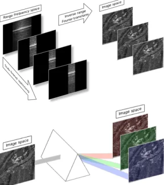
In place of targeting high range resolution, one can also take advantage of wide band to split it in sub bands and generate several lower resolution images from a single acquisition, each being centred on a slightly different frequency. This processes named Multi Chromatic Analysis (MCA) [1] or Split Band corresponds to performing a spectral analysis of the SAR image (Fig. 1).

Figure 1: Split band schematic explanation Above: Spectral decomposition in the spectral domain

below: Spectral analysis in the image domain Split-Band SAR interferometry (SBInSAR) is based on this spectral analysis, allowing to generate several InSAR pairs of lower resolution from a single one. Each sub-band interferometric pair leads to an interferogram generated with its own frequency (or wavelength). Scatterers keeping a coherent behaviour in each sub band interferogram show a phase that varies linearly with the carrier frequency, the slope being proportional to the absolute optical path difference. Therefore, Split Band processing can be used to compute on a pixel-by-pixel the absolute phase, and consequently to perform phase unwrapping [1, 2, 3, 5] as well as ground height retrieval.

The developed SBInSAR processor uses already coregistered interferometric pairs. It splits each image in the spectral domain in a given number of sub-bands to generate a given number of sub-images and associated interferograms. From this stack of interferograms, linear regression is conducted in each point to derive the phase slope that is proportional to the absolute phase. This can be easily understood expressing the interferometric phase with respect to ν, the carrier frequency (Eq. 1) [1]:

Δϕ =4π

λ

(

)

c

(

)

In equation 1, (rs – rm) is the optical path difference and

c the speed of light. Indices m and s refers to master and slave images. Consequently, the interferometric phase, in case of perfect coherence, is a linear function of the optical path difference we are looking for. Finding the slope through a linear regression lead to the absolute optical path difference. If willing to recover the absolute phase, we just have to multiply the found phase slope by ν0, the central carrier frequency of the full bandwidth

signal.

The developed Split Band InSAR (SBInSAR) processor performs linear regression on any points and issues the absolute phase, the corresponding local height and several figures of merit, which are the RMS error on the regression, the correlation coefficient R2, the RMS (one sigma) error on the intercepts and the spectral coherence. The RMS on the intercept is of prime importance because it gives the effective accuracy of the derived absolute phase. It has to be better than a phase cycle to grant to have found the absolute phase fringe number. Classical interferometry can then give the fractional part of the phase. In this way, if two distant points have an RMS error on the intercepts better than a fringe, their absolute phase difference can be computed, allowing to connect them even if separated by non coherent regions. Spectral coherence is computed as the autocorrelation coefficient of the interferometric phase along the sub band interferograms, corrected for the found phase slope.

3. CO-REGISTRATION PHASE

Equation 1 is valid for non-coregistered images. In case images are already coregistered, SBInSAR processing will allow recovering the optical path difference related to the co-registration error (see annexe A).

Whatever the way co-registration is implemented, it is always approximated. Co-registration can be written as: (2) Where Δr is the applied co-registration and ec is the co-registration error. Therefore, the phase slope measured through SBInSAR processing will be:

(3) Consequently, SBInSAR processing may be used to improve range co-registration through the measurement of local co-registration errors.

If willing to recover the full optical phase path, one rs= rm+ r + ec

@' @⌫i

= 4⇡ c ec

have to re-add applied registration Δr. Or in terms of phase, one has to re-add the co-registration phase:

(4) 3.1. TanDEM-­‐X  case  

In the case of TanDEM-X bistatic image pairs, images are provided already co-registered. Co-registration information is provided within the CoSSC data format, which is the one of TerraSAR-X bistatic images pairs. The information is provided as a mesh of range and azimuth co-registration values.

Mesh co-registration values are found using three methods in sequence [6], each one improving the co-registration accuracy. If a method fails, the preceding value is kept without further improvement. The first method computes the co-registration values using precise orbit information from the two satellites and an external DEM. Second method is based on incoherent cross correlation of image patches (correlation of amplitude image patches). The last method is based on coherent correlation of image patches (local coherence optimization). The second and the third method use a correlation threshold and a correlation peak width criterion to assess or reject the found co-registration value.

The mesh of co-registration values has a regular interval of 64x64 full resolution pixels with respect to the master image and the point [0;0] of origin of the mesh corresponds to the point of origin of the master image. Applied co-registration values at any point are found through an interpolation of the four corner values of the mesh cell the considered point belongs to. Taking the formalism as depicted in figure 2, the interpolated registration value V at a range – azimuth coordinate in the mesh reference system (i + Δi ; j + Δj) is given by:

(5) Where Δi and Δj are the fractional distances of the considered point with respect to the mesh cell origin.

Figure 2: Schematic representation of a cell of the mesh of registration values

Handling of co-registration information from TanDEM-X bistatic data was implemented within the SBInSAR processor.

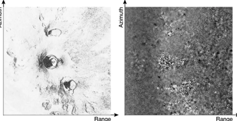
Figure 3 shows the Nyiragongo test site aside with the co-registration phase computed from the co-registration values obtained interpolating the range co-registration mesh provided with the July 21, 2012 bistatic TanDEM-X acquisition.

One can clearly see the grainy aspect of the co-registration phase (corrected for the orbital phase) and so of the co-registration values due to the different method used in the co-registration values computation. On layover, shadowed or too steep slopes areas, only the coarse co-registration values obtained using an approximate external DEM where kept, leading to co-registration values with a higher variance.

4. SBINSAR PROCESSING

SBInSAR processing was performed on the July 21 TanDEM-X bistatic pair. The processor computes the correcting phase term (Eq. A7) as also the accuracy of the linear regression. On figure 4, one can see the derived correcting phase term that must be added to the co-registration phase to lead to the absolute phase. The derived correcting phase term is shown in figure 4, in line with the estimated spectral coherence.

Where spectral coherence is low, RMS error on the SBInSAR measurement of the correcting phase term is high. But, in areas where the spectral coherence is high, confidence interval on the measurement is better. In these areas, we can also observe a grainy aspect of the derived phase. A closer observation shows that the correcting phase term appears in many places as a negative of the co-registration phase term, which is logical since the correcting phase term may also be seen as a local co-registration correction.

'( r) = 4⇡ c ⌫0 r

V(i+ i;j+ j)= (1 j) i V(i+1;j)+ (1 i) V(i;j)

Figure 3: Nyiaragongo test site (left) and corresponding co-registration phase (right)

Figure 4: SBInSAR processing of the Nyiragongo test site Left: Spectral coherence – Right: Correcting phase term When summing both the registration and the correcting

phase term, we obtain the measured absolute phase. Figure 5 shows the derived absolute phase with the estimated RMS error on the intercepts in the linear regression. The shown absolute phase was filtered using a 5x5 pixels moving average window. Computed average was weighted with respect to the inverse of the RMS error on the intercepts in order to give more weight to low error points.

We observe that the grainy aspect of both the registration and the correcting phase terms disappeared in their summation, confirming well that the correcting phase term is first a co-registration correction.

One can clearly see that the bottom platform P3 inside the crater of the Nyiragongo is shown with a phase corresponding to a lower altitude with respect to the crater borders. This shows that the method in itself is working; however not with a sufficient accuracy. If we have a look to the histogram of the RMS error on the intercepts (fig. 6), we observe that no or very few points offer the sufficient accuracy to obtain almost the absolute fringe number within the interferogram. The average error is of about 20 radians (about 3 fringes). Since the altitude of ambiguity is ~41m for the used TanDEM-X bistatic pair, the average 1σ height error is

of about 130m.

Figure 5: RMS error on the intercept (left) and absolute phase (right) issued from the SBInSAR processing of

July 21, 2012 TanDEM-X bistatic pair of the Nyiragongo.

Figure 6: Histogram of the RMS error on the

intercepts (in radian)

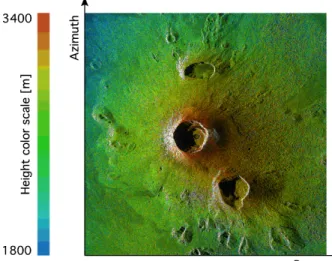
It must be noted that, if the method is not accurate enough for obtaining the absolute fringe index of a point, it can certainly be used to improve the range co-registration locally with a very good precision. The average precision of 3 fringes corresponds in terms of co-registration to an accuracy of three times the wavelength (bistatic case), it is to say of about 10 cm. The derived “absolute” phase may be converted in “absolute” heights (fig. 7). Despite the relatively poor accuracy, performing a weighted average with respect to spectral coherence, height difference between crater rim and lower crater platform P3 was estimated to be of approximately 408m, which is very close to the observed value at the considered acquisition date (400m).

Consequently, we showed that, in its principle, the method is working. But, in the present case, using TanDEM-X data, we cannot derive a phase slope, and subsequently an absolute phase, with a sufficient accuracy across the available bandwidth. Several tests where performed using the three available high incidence TanDEM-X bistatic pairs with different split band scheme (bandwidth and number of extracted sub-bands). Best results were obtained extracting 25 sub bands of 30MHz out of the 100MHz available full band and using a box averaging of 5 x 5.

It is expected that, if data with larger bandwidth would be made available, linear regression would give better results with a sufficient accuracy to lead to an effective absolute phase or fringe index measurement, which should allow connecting independently unwrapped unconnected zones.

5. CONCLUSIONS

We fully implemented SBInSAR processing, including TanDEM-X co-registration data handling. It was shown that SBInSAR applied to already co-registered data allowed obtaining only one component of the absolute phase. The first phase component, called the registration phase, must be computed knowing exactly the registration shift applied to the salve image with respect to the master one. Adding the residual phase component derived through SBInSAR allows getting the full phase on a point-by-point basis.

However, the spectral diversity resulting from the bandwidth (100MHz) of TanDEM-X does not allow getting an absolute phase accuracy better than about 3 fringes in the most favourable cases.

Consequently, if the potentiality of SBInSAR is clearly demonstrated, the nowadays-available bandwidths still not allow getting the required phase accuracy to perform a point-wise absolute phase unwrapping to connect

independently-unwrapped zones, even if the local coherence is high.

It is expected that one can reach the required precision using either TanDEM-X data in pursuit mode or in bistatic spotlight high-resolution mode, the reason why a project was submitted to DLR in answer to the recently launched “TanDEM-X Science Phase Announcement of Opportunity”.

Figure 7: Absolute height map extracted from the

July 21, 2012, TanDEM-X bistatic acquisition on

the Nyiragongo test site

6. ANNEX A

CSL Split Band Interferometric SAR processing (SBInSAR) is starting from already co-registered SAR images. Split band process is then performed on each image of the pair. The fact that the slave image is co-registered to the master image must be taken into account in the computation of the absolute phase issued from the SBInSAR process. In fact, absolute phase is made of two components. The first and most important component is the co-registration phase and the second one is a correction with respect to this co-registration, which is always a local approximation, to lead to the absolute phase.

This correction is obtained through the SBInSAR process while the co-registration phase depends on the way co-registration is implemented.

A way to understand the registration phase is to rewrite split band process under its integral form. In the following, to ease comprehension, we consider that the focused signal has a band-pass square spectrum; it is to say that the point scatterer response is a sinc.

If we consider the generic expression of a sinc response of a scatterer located at distance rm from the sensor, we

have:

(A1) Where:

- ν

is the carrier frequency.

- B is the signal bandwidth.

- c is the speed of light.

- r

is the range position of the considered

scatterer, m standing for master.

Keeping this formalism, the split band signal in the master image may be expressed as:

(A2) Where i is the index of the sub band of bandwidth Bi and centred on frequency ni.

Equation A2 expresses the fact that after band splitting, the focused signal of a given point scatterer at range rm is still a sinc of lower resolution.

Significance given to phase terms is of prime importance. The first phase term is the optical phase and depends on the optical distance between the sensor and the considered scatterer.

The second phase term comes from the split band processing and depends on the spectral shift between the sub band carrier frequency and the full band carrier frequency.

If we consider the slave signal before co-registration, it will be expressed exactly in the same way, simply replacing the m super/subscript with s.

If we now consider a slave signal perfectly an exactly co-registered, the first phase term will stay the same, giving the optical phase with respect to rs, the range distance between the sensor and the scatterer in the slave acquisition.

On the other hand, the second phase term will depend on the location of the phase centre within the

co-registered and interpolated slave image. Since we consider for now perfect and exact co-registration, this location will be rm in place of rs, it is to say, the same pixel location and the same phase centre. Consequently, the second phase term will be identical in both images and will cancel out in the interferometric process leaving only the interferometric phase that will depends on the optical path difference between both acquisitions. Consequently, in case of perfect and exact co-registration, all split band interferograms will be the same and identical to the classical one except a loss of resolution.

This simply means that if co-registration is perfect, the optical path difference is perfectly known too.

Whatever the way co-registration is implemented, it is always approximated. Co-registration can be written as: (A3) Where rs is the range in the slave image, rm is the range in the master image, Δr is the applied co-registration

and ec is the co-registration error. Consequently, after co-registration, the phase centre in the interpolated, or extrapolated, slave image will be located at pixel corresponding to:

(A4)

If we take this error in consideration, from equation A2, the signal in the interpolated slave image may be written:

(A5) The co-registration error only appears in the second phase term and will lead to a perturbation after simplification in the interferometric process. After this latter one, the interferometric phase will be:

(A6) We will thus observe the classical interferogram simply perturbed by a phase term depending on local misregistration and the spectral shift (νi – ν0) between

the sub band carrier frequency νi and the full band carrier frequency ν0.

In split band InSAR, we measure the slope of the phase variation with respect to sub band carrier frequency νi, it S(r) = e i2⇡⌫02crm_sinc ✓ 2 c(r rm) ◆ = e i2⇡⌫02crm Z B 2 B 2 ei2⇡⌫2c(r rm)_d⌫ Sm i (r) = e i2⇡⌫0 2 crm Z ⌫i ⌫0+Bi2 ⌫i ⌫0 Bi2 ei2⇡⌫2 c(r rm)_d⌫ = Bi 2 e i2⇡⌫02crm ei2⇡(⌫i ⌫0)2c(r rm) sinc ✓ ⇡Bi 2 c(r rm) ◆ rs= rm+ r + ec rs r = rm+ ec Ssi(r) = Bi 2 e i2⇡⌫02crs ei2⇡(⌫i ⌫0)2c(r rm ec) sinc ✓ ⇡Bi 2 c(r rm ec) ◆ '_i= 2⇡⌫0 2 c(rs rm) + 2⇡(⌫i ⌫0) 2 cec

is to say:

(A7) So, in place of measuring the absolute phase, we only measure the perturbation with respect to the exact co-registration value. Consequently, SBInSAR applied on a pair of already co-registered images allows getting the local registration error. To recover the absolute optical path, we have to add the applied registration Δr. Or in

terms of phase, we have to re-add the registration phase

Δϕ(Δr) to get the absolute local phase:

(A8) 7. ACKNOWLEDGEMENTS

This work was carried out by CSL, in collaboration with RMCA and MNHN/ECGS under Belgian Government STEREO Contract SR/00/150 in the frame of the Vi-X project (Study and monitoring of Virunga Volcanoes using TanDEM-X)

8. REFERENCES

1. Veneziani, N., Bovenga, F., Refice, A. (2003). A wide-band approach to absolute phase retrieval in SAR interferometry, Multidimensional Systems and Signal Processing, 14, 183-205.

2. R. Brcic, M. Eineder, R. Bamler, U. Steinbrecher, D. Schulze, R. Metzig, K. Papathanassiou, T. Nagler, F. Mueller, and M. Suess. (2009). Delta-k wideband SAR interferometry for DEM generation and persistent scatterers using terrasar-x. In ESA Proc. FRINGE 2009, SP-677.

3. Bovenga, F., Giacovazzo, V. M., Refice, A., Veneziani, N., (2013) Multi-Chromatic Analysis of InSAR data. IEEE Transaction on Geoscience and Remote Sensing, 51(9), 4790-4799.

4. Wauthier C. , V. Cayol, F. Kervyn and N. d’Oreye, (2012), Magma sources involved in the 2002 Nyiragongo eruption, as inferred from an InSAR analysis, J. Geophys. Res., 117, B05411, doi:10.1029/2011JB008257

5. Bovenga, F., Giacovazzo, V. M., Refice, A., Veneziani, N., Derauw, D., Vitulli, R. (2011). Interferometric Multi-Chromatic Analysis of TerraSAR-X Data. In Proc. 4th TerraSAR-X Science Team Meeting, DLR – Oberpfaffenhofen, Germany, 14-16 February 2011.

6. S. Duque, U. Balss, C. Rossi, (2012), CoSSC Generation and Interferometric Considerations, DLR Remote Sensing Technology Institute, TD-PGS-TN-3129, issue 1.0 @ '_i @⌫i = 4⇡ c ec ' = '( r) + '(ec) ' = 4⇡ c ⌫0 r + 4⇡ c ⌫0ec