Learning, teaching and sophistication in a strategic game

HAL Id: dumas-00813551

https://dumas.ccsd.cnrs.fr/dumas-00813551

Submitted on 15 Apr 2013

HAL is a multi-disciplinary open access archive for the deposit and dissemination of sci-entific research documents, whether they are pub-lished or not. The documents may come from teaching and research institutions in France or abroad, or from public or private research centers.

L’archive ouverte pluridisciplinaire HAL, est destinée au dépôt et à la diffusion de documents scientifiques de niveau recherche, publiés ou non, émanant des établissements d’enseignement et de recherche français ou étrangers, des laboratoires publics ou privés.

Learning, teaching and sophistication in a strategic game

Emmanuel Malsch

To cite this version:

Emmanuel Malsch. Learning, teaching and sophistication in a strategic game. Economics and Finance. 2012. �dumas-00813551�

UNIVERSITE PARIS 1

MASTER 2 RECHERCHE MENTION ECONOMIE-PSYCHOLOGIE

L

EARNING

,

T

EACHING AND

S

OPHISTICATION IN A

S

TRATEGIC

G

AME

Présenté et soutenu par : Emmanuel Malsch Date : 12 juin 2012

! "!

« L’université de Paris 1 Panthéon Sorbonne n’entend donner aucune approbation, ni désapprobation

aux opinions émises dans ce mémoire ; elles doivent être considérées comme propre à leur auteur »

SOMMAIRE

INTRODUCTION 4

EXPERIMENTAL DESIGN 11

Game and Incentives 11

Belief Elicitation 14

PRELIMINARY RESULTS 15

“DO I THINK MY OPPONENT CAN BE A LEARNER?” 19

DO PLAYERS USE THE AWARENESS THAT THEIR OPPONENT’S MIGHT BE LEARNERS TO TEACH

THEM? 23

IS THIS TEACHING STRATEGY A WINING STRATEGY? 26

DO PLAYERS SETTLE DOWN ON A “CYCLIC STRATEGY”? 26

CAN WE TALK ABOUT LEARNING OF CORRELATED STRATEGY IN OUR GAME? 27

WHAT ABOUT INEQUITY AND RISK AVERSION? 28

DISCUSSION 29

REFERENCES 31

! #! !

I. I

NTRODUCTION

During a social interaction in a economic context or even in a basic everyday life situation, people do act differently depending if the interaction is likely to happen again in the future, depending on the frequency of this interaction, depending on the utility that people derive from this interaction. The choice they make during these social interactions determines the outcome (both real and expected) of it and these outcomes can be more or less stable in time. If they stabilize in time, game theorist will call it “equilibrium”, the condition of a system in which all competing influences are balanced. For every kind of interaction, there might be one or more possible equilibrium, depending also on the type of equilibrium that we are talking about.

Among the theoretical possible kinds of equilibrium, we can find – among others- the following ones:

- The Pareto efficient equilibrium. In a Pareto efficient economic equilibrium, no allocation of a given good can be made without making at least on individual worse off. It is a minimal notion of efficiency and does not necessarily result in a socially desirable distribution of resources (Fudenberg and Tirole, 1983).

- The Nash equilibrium. Proposed by the Nobel Price John Forbes Nash (1951), it represents a solution concept of game involving two or more players “in which each player is assumed to know the equilibrium strategies of the other players, “in which each player is assumed to know the equilibrium strategies of the other players, and no player has anything to gain by changing only his own strategy unilaterally” (Osborne, Martin J., and Ariel Rubinstein, 1994). If each player has chosen a strategy and no player can benefit by changing his strategy while the other players keep theirs unchanged, then the current set of strategy choices and the corresponding payoffs constitute a Nash equilibrium (a pure-strategy one). Most of the time, the expression Nash equilibrium is a pure strategy Nash equilibrium, meaning that it provides a complete definition of how player will play a game. It allows determining the kind of choice a player will make for any situation he could face.

- The risk-dominant equilibrium (refinement of the Nash equilibrium). A Nash equilibrium is considered risk dominant if it has the largest basin of attraction, meaning the more uncertainty players have about the actions of the other player(s), the

! $!

more likely they will choose the strategy corresponding to it. In other words, it is a risk-avoidance equilibrium (Harsanyi and Selten, 1988).

- The mixed strategy Nash equilibrium (Von Neumann and Morgenstern, 1947). A mixed-strategy is an assignment of probability to each pure strategy. This allows for a player to randomly select a pure strategy. Pure-strategy (mentioned above) is a degenerate case of mixed strategy, in which that particular pure strategy is selected with probability 1 or 0. A mixed strategy Nash equilibrium is a combination of players probability mix of strategy which gives the best possible repartition of decision sets for every single player given the possible repartition of decision set of the other players in the game.

Experimental game theory does a good job at predicting, explaining and modelling these kinds of equilibriums in social or strategic interactions. But how do these equilibrium emerge in games? If they actually do, how do people converge to these equilibriums in real-life social interactions? Do people learn? What are their learning strategies? How do they use them to maximize their utility?

“The question of how an equilibrium arises in a game has been largely avoided in the history of game theory, until recently. Equilibrium concepts implicitly assume that players either figure out what equilibrium to play by reasoning, follow the recommendation of a fictional outside arbiter (if that recommendation is self-enforcing), or learn or evolve toward the equilibrium.” This is how Camerer (1995) starts the chapter on Learning in his book (Behavioural Game theory Experiments in Strategic Interaction). When Camerer talks about equilibrium, he actually means a Nash equilibrium. But again, how do subjects figure out their equilibrium? And again, do they learn with the interaction?

In his book, Camerer defines Learning as “an observed change in behaviour owing to experience.” Following Camerer’s statement, traditionally, Game theory has been focusing mainly on equilibrium analysis in iterated games, especially Nash equilibrium. If we ask ourselves when and why we might expect equilibrium of this kind to arise, the traditional explanation of equilibrium is that it emerges from a complete and serial analysis and introspection by the players in a situation where the rules of the game, the rationality of the players, and the player’s earning functions are all common knowledge. But this answer may have both conceptually and empirically many problems.

! %!

First, there might be a problem in situations where there are multiple equilibriums. What makes the subjects a given equilibrium over another? How is this choice different from random? Stated differently, what mechanisms underlie the subjects choice of the same equilibrium? How does a specific procedure of coordination of players’ expectations (Harsanyi and Selten, 1981) come to be common knowledge?

Second, there is still doubt that the hypothesis of exact common knowledge of payoffs and rationality apply to many games. If we do reduce the assumption of “common knowledge” to “almost common knowledge”, we might weaken the conclusions of what we predict, analyze or model through our experimental or theoretical setups.

Third, equilibrium theory predicts poorly early rounds results of most experiments, even if it does better in later rounds. For example, it takes a while for subjects to realize in a simple public good game that the Nash equilibrium (their utility maximization strategy) is to contribute nothing. This move from non-equilibrium to equilibrium play is difficult to explain with purely introspective theory.

While some studies have been looking at the theoretical side of the question by analyzing the convergence supported by evolutionary forces or adaptive rules, other studies have been using experimental data to examine in a more accurate way the player’s behaviour. Experiments are a good way to test models of learning because we can control how payoffs and information affect interactions in games. It’s a good way to observe and analyze what subjects know (and know others know, and so on), what they expect to earn from different strategies, what they have experienced in the past, and so forth.

The present study is clearly based on the latter idea.

There are many approaches to learning in games:

- Evolutionary dynamics. It assumes that a player is born with a strategy and plays the same strategy all over again, no matter how much repetition. The more successful the strategy, the longer the player survives or the more he reproduces.

- Reinforcement learning. One step further to evolutionary models in the cognitive sophistication is the idea that agents might reinforce their previously played strategy looking at their last payoff.

- Belief learning models assume that players update their beliefs about the other’s strategy by examining their opponent’s past behaviour and identifying the best one.

! &!

players keep track of what has been played in the past and use these records to determine their future strategy in the upcoming periods.

At the opposite, there is Cournot best-respond dynamics: he assumes that players only look at the most recently played strategy of the opponent, think that it will be played again and determine their best-response based on this last observation.

Weighted fictitious play model (Cheung and Friedman, 1997; Fudenberg and Levine, 1998) assumes a hybrid form of the Fictitious play and Cournot models. Players might actually mix these two strategies, maybe looking only at a given number of last observed opponent’s choices, applying different probabilities of future realization on them. The belief held by player i about the probability that player j will play action a in round t+1 is given by:

˜ B i a (t +1) = Id a_j( )= at ( )+ " u u=1 t#1

$

Id a_j(t#u)= a ( ) Id + "u u=1 t#1

$

where Id a_j( )= at

( ) equals one if player j has played action a in round t, and zero

otherwise. Actions played in a given round are discounted with time at rate " " 0,1

[ ]

. As stated above, when " = 0, this model reduces to Cournot Learning, where the belief held in period t about action a is one if the action has been played in round t-1, and zero otherwise, while when " = 1, the model reduces to fictitious play, where the belief about a given action corresponds to the frequency with which this action has been played since round 1. The Cheung Friedman model has been found to perform well empirically to explain people’s behaviour in games.

- Experience-weighted attraction (EWA) learning is Ho’s and Camerer’s (1999a) model combining elements of reinforcement theories and weighted fictitious play. The model adds an element to reinforcement and belief learning, the weight players give to forgone payoffs from non-chosen strategies. If this weight is very low, it means that the player’s strategy reduces to a simple version of choice reinforcement, whereas when the weight is very high, the player’s model of decision reduces to a weighted fictitious play.

- Imitation. People learn by imitating the others behaviours. It is not necessarily payoff dependent (imitation of the successful opponent/player).

- Sophisticated (anticipatory) learning. In adaptive models such as fictitious play or EWA, players only look back at the previous history of the game interaction. This

! '!

means that players will never act differently from before or from what they expect. Their beliefs are based on what they have previously observed. “They will also ignore information about other player’s payoffs” (Camerer, 1995). But a lot of studies show that players do care about other player’s payoffs. Anticipatory learning models or sophistication overcome these limitations (Selten, 1986; Camerer, Ho and Chong, 2002a; Stahl, 1999a). Camerer et al. (2002) assume a population composed of fully rational players (having the ability to play equilibrium behaviour) and adaptive ones who only look backward to choose their current action, and adds sophistication to adaptive models. Of course, rational players have in mind their own estimation of the repartition (not necessarily the real one) between rational and adaptive players, using their knowledge to outguess their adaptive opponents. They observed that “players do use information about other’s players’ payoffs to reason more thoughtfully about what other players’ payoffs will do in the future.” Players might form beliefs and best respond according to them but the true originality is that players don’t just think that their opponents will basically reproduce the same patterns of behaviour (as if they were myopic).

- Rule learning. This model assumes that players use decision rules that transform histories into strategy choices. They determine through the game process which rules rather than which specific strategy to use. These rules can be all of those listed above and others like tit-for-tat (answering the same or opposite way the opponent(s) did in the previous period), level-k reasoning, the idea of this latter theory is that people do possess different level of reasoning abilities and that the more reasoning levels you get, the more you are able to predict the level of reasoning of your opponents (Stahl and Wilson, 1995) and choose your strategy accordingly.

Most of the reviewed literature (except for the sophistication model) about theories of learning considers the player as myopic and purely adaptive, taking their decisions based almost entirely on their past experience and based on the assumption that their opponent follows an exogenous process, as if he was a kind of machine, pre-programmed to react in a given way to a given strategy. As a consequence, such myopic players might never take into account the effect or influence of their own actions on their opponents’ future behaviour. This statement might lead to think that strategic interaction in games do not matter for players, which seems quiet a strong assumption. The other way of thinking, that players might only

! (!

behave within the frame of full rationality (Nash equilibrium player), is another kind of extreme. There might be an explanation between these two extremes.

What if for example we observe a rational player surrounded with other players who learn only from personal experience, like in Ellison’s (1997) paper? He shows that the learning process naturally generates contagion dynamics, and that the rational player has an incentive to act non-myopically and with patience to move the whole group to a new a risk-dominant equilibrium (see above).

On the contrary, Offerman et al. (2001) found that player’s belief formation doesn’t take into account strategic interactions. However, the authors highlited that the public good game they used in their experiment is strategically complicated, namely that a funding threshold has to be reached before the good can be provided. The game has also multiple equilibria so that the players are cognitively highly stimulated and it makes the strategic reasoning very difficult. Huck et al. (1999) found that players tend to imitate the others and that “imitation might be the unique learning rule that prevents human players from teaching their opponents”. But in other experimental environments, players have proven to be more sophisticated (far-sighted) and use their actions not only to optimize their immediate pay-off as myopic players would do but also to manipulate (or teach) their opponents’ behaviour in order to reach preferable outcome in the future.

Hyndman, Terracol and Vaksmann (2009), while studying teaching in coordination, show that teaching represents an investment according to which players might postpone immediate payoffs by playing sub-optimal actions in order to manipulate their opponents and get more in the long-run by leading the other players to a preferable equilibrium, and this especially when teaching incentives are high and teaching costs are low. Terracol and Vaksmann (2009) also identified the role of teaching on convergence to a pure strategy Nash equilibrium in fixed matching environments.

The present study would like to show – among other things - in the spirit of Hyndman, Terracol and Vaksmann (2009), that learning and teaching are still observed in an environment where there is no pure strategy Nash equilibrium (but still, as in any finite game, a mixed strategy Nash equilibrium), which is the case in the majority of real-life situations.

! )*!

The main objective in this paper is to test experimentally the following hypotheses:

- First, we want to know if players believe that their opponents can be learners and that their actions might influence their opponent’s beliefs.

- Second, we would like to investigate the idea that players do use this awareness of their opponent’s ability to learn to manipulate their opponents’ beliefs.

- Third, we want to know if there are other explanations we can provide for the way players behave in our game: “cyclic behaviour”, “learning of correlated strategies”? - Last, we think that Inequity and Risk aversion might play a role but that doesn’t

undermine our teaching strategy hypothesis mentioned above.

The paper is organized as follows. Section II introduces our game and experimental procedure. Section III gives some preliminary results and descriptive statistics. Section IV-V and VI shows that subjects might be more sophisticated than the standard theories predict. Section VII-VIII-IX explore the possibility of “cyclic playing behaviours”, the existence of a learning of “correlated strategy” and examines the effect of “inequity and risk aversion”. Section X concludes the paper.

! ))!

II. E

XPERIMENTAL

D

ESIGN

1.

Game and Incentives

In order to examine the emergence of teaching, an experimental session was conducted using a 2 x 2 matrix game. 26 inexperienced subjects (12 female subjects) aged between 22 and 65 years were drawn randomly at the library of the University of Paris 1 Pantheon-Sorbonne (Maison des Sciences Economiques) and from outside the University and were asked to play the game presented in Figure 1 for a total of 20 periods (the game stayed the same along all periods). Let’s take an example to explain the following matrix. On period one, if Player 1 selects strategy A and Player 2 selects strategy C, the outcome for Player 1 is 80 and the outcome for Player 2 is 20. If Player 1 selects strategy B and Player 2 selects strategy C, the outcome for Player 1 is 100 and the outcome for Player 2 is 25, and so on. Every combination has respectively 2 outcomes for both players.

In order to give the best chance for teaching to emerge, subjects were put in fixed pairs for the entire experiment and this information was clearly stated in the instructions (see Appendix). We voluntarily took a non-symmetrical pay-off matrix and lower payoffs for Player 1 and 2 in order to avoid interaction effects between the players when observing learning and teaching. All this will be explained further in this paper.

Player 2

Strategy C Strategy D

Strategy A 80, 20 60, 15

Player 1

Strategy B 100, 25 40, 30

Figure 1. Payoff matrix

Before each experimental session began, subjects were randomly assigned the role of either Player 1 (row player) or Player 2 (column player) and were told that they would remain in that role for the entire duration of the experiment. We had to do every experimental session one at a time for material reasons. Subjects were put in front of each other with only one computer. The game was presented on a Microsoft Excel file (Figure 2 and Appendix). No talking was allowed during the entire duration of the experiment.

! )+!

Player 1 had to fill-in his answers for the first period, click on a button, which would present a neutral page and turn the computer so that the other player could use his own playing interface, and so forth. This procedure could guarantee that the players were playing the game simultaneously, ignoring what the other player was playing in the on-going period. After the first period was over, both players would see the outcomes of the previous period. Anytime, both players could also see their own choices and previous opponent’s choices along the entire history of the game. Subjects were told the experiment would last not more than 30 minutes.

Figure 2. Excel file of the experiment

On average, the experiment’s duration was around 45 minutes, 2 pairs of subjects took more than 1 hour to understand the experiment and go through the game.

There was no fixed participation fee. Subjects were told that they were 2 player types: Player 1 and Player 2. They were also told that there was no competition between the two actually playing subjects. They were notified that the minimum possible payoff of Player 1 was greater than the maximum possible payoff of Player 2. They were also told that if they best

! )"!

performed among the players of their type (Player 1 or Player 2 type), they would be rewarded 5!. They didn’t know the subjects who belonged to their type. Subjects earned on average 72 ECU (SD= 22,21) (Experimental Currency Unit) inside the Player 1 type and 22 ECU inside the Player 2 type.

A translation from the original French instructions given to the subjects can be found in the Appendix. In addition, subjects received an oral summary of the experimental conditions detailed in the instructions and questions were answered before the experiment began.

Notice that our game has no pure-strategy Nash equilibrium and one mixed-strategy Nash equilibrium. The mixed strategy Nash equilibrium was {(0.5,0.5);(0.5,0.5)}. (see definition of mixed strategy Nash equilibrium above).

Note that one desirable feature of our design is that, since there is no pure-strategy Nash equilibrium and since players aren’t in competition, subjects have to choose the best-response strategy given their beliefs about the strategy of others. Player 1 types have a bigger incentive for playing their maximum payoff strategy than Player 2 types (strategy B, payoff 100, if strategy C is selected by Player 2). But they face the risk that Player 2 type might shift to strategy D to maximize his own payoff (strategy D, payoff 30, if strategy B is selected by Player 1). Given the nature of the payoff matrix.

Under the hypothesis of risk neutrality, Player 2 could want to minimize his risk of getting the minimum payoff (15 if Player 1 plays A) and try to get either 20 or 25 most of the time. On the other side, Player 1 anticipating (sophisticatedly) the previous Player 2 strategy might want to try to teach his way to his maximum payoff (100 if Player 2 plays C). Player 1 should play strategy A at the beginning of the game in order to force Player 2 to play his “safe” strategy C. Once this is done, after a few periods, he should shift to strategy B and earn his maximum payoff, creating a stable strategy combination (B-C). This is the kind of behaviour that we define as teaching. More precisely teaching is best thought of as an investment: the successful teacher will incur short-run costs (80 for an A-C combination) in order to obtain a long-run gain (100 for an B-C combination).

Note, however, that in order to study teaching, we also need teachers (Player 1) to be paired with subjects who are capable of being taught (e.g., an adaptive learner, Player 2). In order to do this in our game, we kept the shifting incentives of Player 2 very low (5), moreover, the incentives that the Player 2 had to engage in long-run behaviour were always lower than those of the Player 1 (5 for Player 2, 20 for Player 1).

! )#!

If both players converge toward the mixed-strategy Nash equilibrium, we should observe a 25% repartition in all four cells of the payoff matrix (25% for A-C, B-C, A-D, B-D).

At the end of each session, the experimenter asked separately to all participants what was their strategy. We will describe some of them later in the paper.

2.

Belief Elicitation

The aim of the present study is to examine the player’s propensity to play sub-optimal strategies during a possible teaching phase. For this examination to be possible, we need to observe the difference – if there is a difference – between what subjects believe and what they really play given these beliefs, and what outcome do they get. Following the work of Nyarko and Schotter (2002), Hyndman, Terracol and Vaksmann (2009), we had to elicit player’s beliefs to precisely determine their best response at each time. In each round, subjects had to perform two kinds of actions:

- First, they were asked to report what they thought their opponent would do during the current period with a probability question. “On a scale from 0 to 100, what is the likelihood that your opponent will play strategy A and B (C or D) if Player 1 was asked the question)?

- Second, after answering the above question, they had to choose their action A or B (C or D), depending on their Player type.

Beliefs were rewarded for accuracy according to the following quadratic scoring rule, which should induce truth-telling if subjects are risk neutral:

8_{" 4 1 " b} a

(

)

2+ b_z2 z#a

$

(

)

% & ' ( ₎ *

If their belief were close to what their opponent did during the on-going period, they could earn a maximum of 8 points. If subjects’ prediction were completely wrong, they would get 0 points for their prediction. Let’s take an example. If Player 1 predicts that Player 2 will play strategy C with 100% chances, and Player 2 actually plays strategy C, than the pay-off derive from the above function is P = 8 – 4 (1-100%)2

+(0%)2

= 8.

We tried to keep the reward reporting beliefs small in comparison with the payoffs associated to the game so that players could not use their belief payoff as a “hedge” against potentially low payoffs. At the end of each round, subjects were informed about the action of their opponent, their game payoff, their prediction payoff and the game payoff of their opponent for the current round. Again, during the whole experiment, subjects could see the entire

! )$!

history of actions and stage game payoffs as well as their predictions in earlier rounds, but not their prediction payoffs from earlier rounds.

III. G

AME OUTCOME

C

OMBINATIONS AND

P

RELIMINARY RESULTS

We will begin our analysis of the experimental results with a brief look at the combination outcomes combination of the game.

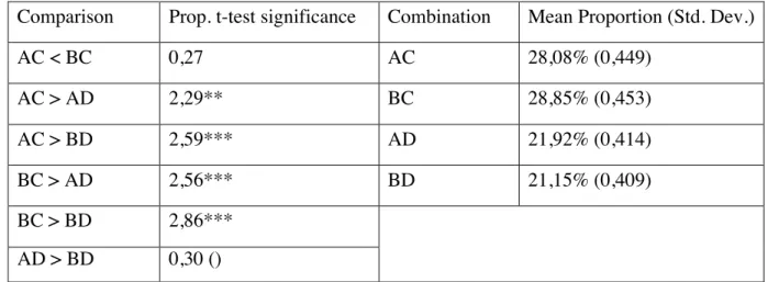
Comparison Prop. t-test significance Combination Mean Proportion (Std. Dev.)

AC < BC 0,27 AC 28,08% (0,449) AC > AD 2,29** BC 28,85% (0,453) AC > BD 2,59*** AD 21,92% (0,414) BC > AD 2,56*** BD 21,15% (0,409) BC > BD 2,86*** AD > BD 0,30 ()

*10% level of significance; ** 5% level of significance; *** 1% level of significance.

Table 1. Comparison of proportions of combinations during the whole game (period 1-20)

For the proportion comparison results, we used a two-sample t-test of proportion. All the results in this table are confirmed by non-parametrical Wilcoxon rank sum test.

Comparison Prop. t-test significance period 1-10 Prop. t-test significance period 11-20 Comb. Mean Proportion period 1-10 (St. Dev.) Mean Proportion Period 11-20 (St. Dev.) AC vs BC 0,20 -0,58 AC 27,69% (0,448) 28,46% (0,452) AC > AD 0,40 2,91*** BC 26,92% (0,444) 30,77 % (0,462) AC > BD 2,28** 1,40 AD 26,15% (0,440) 17,69% (0,382) BC > AD 0,20 3,48*** BD 19,23% (0,395) 23,07% (0,422) BC > BD 2,08** 1,98** AD vs BD 1,88** -1,52*

*10% level of significance; ** 5% level of significance; *** 1% level of significance.

! )%!

Let’s look at each possible outcome combination (see Figure 1), try to give a hypothetical meaning to every four of them and see if we find some evidence in our descriptive statistics above:

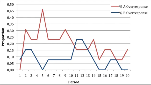
- BD combination: BD gives the maximum outcome (30) to Player 2 but is Player 1’s minimum outcome (40). There is a risk for Player 2 to play this strategy because Player 1 will systematically try to move to AD in order to increase his payoff (to 60). As a result Player 2’s risk is to get his minimum outcome (15) after BD was played. It might be interesting to point out the fact that BD is also an inequity aversion combination. Even if subjects knew they were not in competition with each other, a few of them reported to be surprised by the fact that the other player would always – whatever the situation – earn more then them. In our data (see Table 1), BD shows up 21,15% of the time and has significantly the lowest proportion of combination compared to the other combinations (except for AD).

Figure 3. Comparison of played combination for AD and BD.

- AD combination: AD is the worst combination for Player 2 and as such, he might not want to stay very long in this situation. Player 2 could try to shift to C in order to increase his payoff by 5 ECU or try to teach his way to BD again, this being very unlikely since playing D makes the Player 2 dependent of Player 1’s decision. AD is the third most played combination in the game and is significantly inferior to AC and BC in terms of proportion. When looking more closely at the data (see Figure 3), we

*! +! #! %! '! )*! )+! )#! )%! )'! )! +! "! #! $! %! &! '! (! )*! ))! )+! )"! )#! )$! )%! )&! )'! )(! +*! # $% & ' ( !) * + , -.% /-* .0! #'1-*(! ,-! .-!

! )&!

see that AD is a transition combination. Each time we observe an increase in BD, almost in the next period, we observe an increase in the AD combinations.

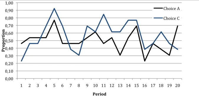
- AC combination: AC is risk aversion combination for both players. If Player 1 plays AC and try to teach his way to BC, he faces the risk of Player 2 trying to teach his way to BD and so on, returning back to the original position AC after four periods. Player 2 is better of playing column C because he secures a mean outcome if Player 1 plays randomly A or B. During the debriefing phase, subjects do report that they played AC combination because they felt it was the better way to secure this mean outcome. In our data, we can see that AC and BC are the most played combination, statistically significant at more than 1%, especially in middle of the first and last 10 periods of the game (see Table 2 and Figure 4). We can observe this pike at period 4-5-6 and the same pattern at period 14-15-16. In the figure 4, just visually, we might find the first raw evidence that at this point Player 1 may have tried to teach their way to the BC combination by over-playing AC. This pattern is confirmed by the fact that AC and BC show almost the same proportion during the whole game. In the first 10 periods, combination AC is more played than combination BC and this tendency is reversed in the last ten periods. Statistically speaking, these differences are not significant but we need to remind our reader that the number of subjects is 13, this effect might be confirmed significant with more observations and a more refined experimental design.

Figure 4. Comparison of played combination for AC and BC.

*! +! #! %! '! )*! )+! )#! )%! )'! +*! )! +! "! #! $! %! &! '! (! )*! ))! )+! )"! )#! )$! )%! )&! )'! )(! +*! # $% & ' ( !) * + , -.% /-* .0! #'1-*(! ,/! ./!

! )'!

- BC combination: BC is the best combination for Player 1. His motivation (teaching incentive?) to reach this outcome is higher than Player 2’s motivation to reach his (100 vs. 30). Our idea was that the BC combination would be the next step (the more played combination) after AC. After playing A for a while, Player 1 should normally try to get to his maximum outcome shifting to from AC to BC, overcoming the risk (teaching cost?) of Player 2 trying to shift upon BD. This might be the teaching investment we have been evoking earlier in this paper. If we look closely at the figure 4 (above), we might find that the pikes of BC combination follow very closely the pikes of AC combination (especially period 8-9 after the big pike of AC combination, and also period 13-14 and period 16-17-18). Again, in order to observe a statistically significant difference, we might increase the number of subjects and also the number of periods. We will discuss these limits of the experimental design at the end of this paper.

Teaching cost and teaching incentives are both notions reported by Hyndman, Terracol & Vaksmann (2009). They have been manipulating these variables showing that the more the incentive and the less the cost of teaching, the more teaching they observe. We are going to seek for a confirmation of these results in the next sections.

! )(!

IV. “D

O

I

THINK MY

O

PPONENT CAN BE A LEARNER

?”

Before even mentioning teaching strategies, we need to be sure about the fact that subjects are aware that their opponent might learn from their previously played strategies. Indeed, if the teacher believes his opponent updates his actions largely due to the observed history of play, and that he updates sufficiently rapidly, then he might be willing to make the required short-term investment in order to make his way through his best combination. In this section, we examine whether players beliefs are influenced by their own actions or see their opponents as learners. Our idea is to see if subjects believe they can influence their opponents through their own choices. This implies in the spirit of Terracol and Vaksmann (2009) “an investigation of players’ belief formation process to check whether they take into account the influence brought by their own past actions when forming beliefs about their opponents’ behaviour at a given time”.

This means we want to see if subjects view their opponent as an adaptive learner who is capable of being taught something.

We are not interested in modelling the way player’s action might influence his opponent’s behaviour, we just need to show that there might be a belief that teaching is possible.

If we ask ourselves how players build their beliefs, along the work of Hyndman, Terracol & Vaksmann (2009), two elements might come to our mind:

- First, we need to check if players do look at the past history of action of their opponents to form their beliefs, and if this has an effect on their prediction (the answer to the belief elicitation question). This first element will be integrated in our regression model as a “history of action” variable, expressed as the observed frequency of choices made by the opponent, under the hypothesis that player’s behaviours follow the fictitious play model. - Second, if players think they can influence (teach) their opponents’ action, they might

also take into account the effect of their own last actions when they answer to our belief elicitation question. This second element will be integrated in our regression model as a “last action” variable (in t-1).

! +*!

Our two elements is expressed through these following formulas:

Bit = F historyofaction

(

1" t #1,lastactiont #1

)

ˆ

B it = G historyofaction

(

1" t #1

)

D_it = Bit # ˆ B it

B_{it represents the effect of the combination of history of action and last action variables}

regressed on the prediction of the opponents choice. ˆ B _{it represents the effect of the history of}

action variable alone regressed on the prediction of the opponents choice.

D_{itis the difference between the two first presented elements, basically the part of the}

prediction unexplained by the “history of choice” variable. If the last action variable

demonstrates a significant effect in our model, we might conclude that the player may take into account his own action in the prediction of his opponent action and in a next step, might also try to influence his opponent’s beliefs.

To operationalize this model with our data, we run two OLS regressions along the following formulas:

Player 1’s prediction over Player 2’s current choice C estimation: Equation (1)

B_C

t ="0+"1actAt#1 +"2freqC0$ t #1+%it

B_C

tis our dependant variable, the prediction by Player 1 that Player 2 will play C during the

current period. "₁act A_t

#1represents Player 1’s last action A and "2freqC0# t $1 Player 2’s

observed history of action C observed by Player 1 (independent variables).

Player 2’s prediction over Player 1’s current choice B estimation: Equation (2)

B_B

t ="0+"1actCt#1+"2freqB0$ t #1+%it

B

Btis our dependant variable, the prediction by Player 2 that Player 1 will play B during the

current period. "₁act

Ct_#1represents Player 2’s last action C and "2freqB0# t $1 Player 1’s

! +)!

Our estimation results of Equation 1 and 2 are collected in Table 3.

B Ct Coef. (SE) B Bt Coef. (SE) act A_t "1 -8,17* (4.377) act C_t "1 6,32 (4,839) freqC_{1" t #1} 0,45*** (0,096) freqB_{1" t #1} 0,576*** (0,081) cons. 37,77*** (6,238) cons. 20,28*** (5,382) 10% level of significance; ** 5% level of significance; *** 1% level of significance. Robust standard errors in parentheses. The number of individuals is given in Table 1, each individual played 20 periods.

Table 3. Regression model.

The above results show that their is a significant correlation between prediction of Player 1’s (he) prediction about Player 2’s (she) choice and his last action. Our analysis shows some consistency with our hypothesis that Player 1 (prediction B_Ct) perceives their own past actions (actAt-1) as significantly likely to influence their opponent’s current and future actions. This is

not the case for Player 2’s behaviour. The last action of Player 2 plays no significant rule in the prediction B_Bt (prediction that Player 1 will play strategy B during the current period).

However, we need to emphasize the fact that we found a puzzling result about the sign of the last action (actAt-1) variable, which correlation is negative. This means that the more Player 1

plays strategy A, the lower his prediction of Player 2 playing strategy C. We can try to explain this negative sign (which is definitely positive for Player 2’s equivalent prediction about Player 1 playing B) by the fact that Player 1 might not be so confident with the fact that his last action will influence his opponent in the long run and he might integrate this idea in his prediction.

Another alternative explanation might rely on the experimental conditions that were used, clearly not as strict as what is expected in the standards of experimental literature. After debriefing, subjects were not always very confident at the beginning of the game with the “prediction” question they were asked for. We are conscious of the serious problem this result might be for our work and we will have to investigate this effect deeper in further research.

We may conclude (with caution) that players think their opponents modify their behaviour according to the history of the game, and take this into account in their own beliefs; in other

! ++!

words, subjects realize that their opponents can learn, which is necessary for teaching to even be possible. This shows that players might take strategic interactions into account and form beliefs in a more sophisticated way than the adaptive way postulated by usual proxies. We might have highlighted a sophistication bias1

(Hyndman, Terracol, Vaksman, 2009) in classical proxies used to describe player’s belief-formation process.

Note that we do not assume that players necessarily base their beliefs on the history of their opponents’ play, but rather allow for the possibility of such a belief-formation process.

!!!!!!!!!!!!!!!!!!!!!!!!!!!!!!!!!!!!!!!!!!!!!!!!!!!!!!!!

)_{!the fact that subjects believe that their past actions influence their opponent’s current decisions}

! +"!

V. D

O PLAYERS USE THE AWARENESS THAT THEIR

O

PPONENT

’

S MIGHT BE LEARNERS TO TEACH THEM

?

The previous section highlighted that in our game there is a scope for teaching. The next question we are asking is whether player, particularly Player 1 given their stronger incentives, use their awareness of the belief-formation process to manipulate their opponent’s belief and influence or teach their way to their best outcome.

In the belief-learning literature, players are thought to take a stochastic best response to their beliefs. If we take this idea into consideration, choices which are not a best response to beliefs may be called errors. However, if subjects are trying to teach, then they are taking a statistically sub-optimal action (predicting that their opponent will play C and still playing A while they could have played B to maximize their payoff), expecting that their maximum payoff combination will emerge at some point in time.

In order to capture this sub-optimal action, we need to identify the player’s choices according to whether or not they were playing a best response to stated beliefs. We say that a player “over responds to C” whenever he chooses A despite the fact that B is a best response to his stated belief C. If our subjects are the teachers we expect them to be, they would over respond to A much more frequently than they over respond to B.

Since we are not able to say that Player 2 might act as a teacher (see previous section), we are going to focus on the results of Player 1 type.

Indeed, this is precisely what we see concerning Player 1. If we compare the over-response rate between A and B, we find that Player 1 over-respond A 19,23% of the time and B 8,46% of the time and that this difference is highly significant (two sample test of proportion, value < 1%). Over-response rate A is also superior to over-response rate C (significant, p-value < 10%).

It is hard to interpret such strong tendencies to choose A when B is a best response as errors since it would mean that our subjects are making quite costly errors with considerable frequency. The comparative statics are consistent with our earlier hypothesis of teaching behaviour for Player 1.

! +#!

Figure 5. Comparison of proportion of over-responses A and B.

Besides, if we look at the Figure 5, we can see that this tendency to over-respond A is diminishing over time, meaning that the Player 1 might have tried to teach his opponent during the first 10 periods and seeing that his teaching strategy had no effect, he might have abandoned it in the last 10 periods. If we compare the over-response rate between A in the first 10 periods (24,61%) and in the last 10 periods (13,84%), we find a significant difference (p-value < 5%), between these two time spans.

Figure 6. Comparison of proportion of over-responses A and C.

*0**! *0*$! *0)*! *0)$! *0+*! *0+$! *0"*! *0"$! *0#*! *0#$! *0$*! )! +! "! #! $! %! &! '! (! )*! ))! )+! )"! )#! )$! )%! )&! )'! )(! +*! # 1 * 2 * 1 /-* . ! #'1-*(! 1!,!234554678964! 1!.!234554678964! *0**! *0*$! *0)*! *0)$! *0+*! *0+$! *0"*! *0"$! *0#*! *0#$! *0$*! )! +! "! #! $! %! &! '! (! )*! ))! )+! )"! )#! )$! )%! )&! )'! )(! +*! # 1 * 2 * 1 /-* . ! #'1-*(! 1!,!234554678964! 1!/!234554678964!

! +$!

If we look at Figure 6, we might find some interesting significant results. Player 1 starts teaching in the first 10 periods and Player 2 waits the last 10 periods to over-respond C (not significant, but again graphically interesting). This result might need further research with more subjects and more experimental design compliance to the standards of the literature.

Our results - the dynamics of over-response - so far provide support for our third hypothesis that subjects try to teach their opponents even if this tendency decreases over time and particularly when the opponent do not react to it. Our results also suggest that Player 2 types take a more passive role and are more likely to be followers.

! +%!

VI. I

S THIS TEACHING STRATEGY A WINING STRATEGY

?

Our first answer to this question is that the players who earned the more ECUs were those who managed to teach their opponent: Player 1 teaching Player 2 to play AC before shifting to the BC outcome.

If we look at the means of earning, we can say that Player 1 types – who have been shown to try to teach their way to their maximum combination in the previous section - earn significantly more than the mixed-strategy Nash equilibrium (one-sample t-test, 72 ECUs (Teach) > 70 ECUs (Nash) with a p-value < 5%). This difference is not significant for the Player 2 types earning.

VII.

D

O PLAYERS SETTLE DOWN ON A

“

CYCLIC STRATEGY

”?

Figure 7. Comparison of proportion of choice A and choice C.

This idea of “cyclic strategy” comes from the fact that players might play a given series of combination during the game that they might informally agree on during the experiment.

If we take a closer look at Figure 7, we can see that Player 2 strongly reacts to Player 1’s choice A with choice C. A pike in choice A correspond most of the time to a pike in choice C. Statistically speaking, where in the first period, there is no significant difference between choice A and choice C, this difference becomes significant (choice C: 59,44% > choice A:

*0**! *0)*! *0+*! *0"*! *0#*! *0$*! *0%*! *0&*! *0'*! *0(*! )0**! )! +! "! #! $! %! &! '! (! )*! ))! )+! )"! )#! )$! )%! )&! )'! )(! +*! # 1 * 2 * 1 /-* . ! #'1-*(! /:8;<4!,! /:8;<4!/!

! +&!

47,54%, with a p-value < 10%). This results show some consistency with the idea that Player 2 might react to the teaching strategy of Player 1 choosing strategy A maybe in order to move to choice B afterwards, which is confirmed by the shift of choice A in Figure 7 from 53% in the first 10 periods (mean proportion) to 47% in the last 10 periods (mean proportion). These last observation are purely speculative, no statistical significance emerged in the data.

An interesting observation of the raw data shows that a few pairs of players show a pattern of combination suites where both Player settle down on a playing cycle, an alternation between BC and BD, playing BC most of the time, but sometimes playing BD. These pairs are also those with the most important earnings. This is what we might call a cyclic behaviour, both players accepting to deviate from their best-outcome for a few periods in order to content each other, without the threat of loosing to much through the process.

VIII. C

AN WE TALK ABOUT LEARNING OF CORRELATED STRATEGY IN OUR GAME

?

The idea of a correlated learning strategy relies on the fact that players might try to approach a dynamic equilibrium during the learning process of the game. This is an hypothesis that we would like to test with our following results.

In fact, Player 1’s mean choice behaviour is to play strategy A and B 50% of the time, this is a significant equality when considered all Player 1’s mean choices. However, Player 2’s mean choice behaviour is to play strategy C 57% of the time and strategy D 43% of the time, this difference being significant at less than 1% level.

It is important to notice that nothing prevents us from saying that players don’t play the mixed strategy Nash equilibrium, but we may find some consistency with the idea that while Player 1 alternates evenly between both strategies, Player 2 playing C more frequently than D, and tries to maximize his minimum outcome (20 and 25), this strategy being the less risky and costly for him. This idea goes against the teaching hypothesis tested above and goes along the theories of Rule learning (Stahl and Wilson, 1995).

We should add that in order for correlated strategies or cyclic behaviour to emerge, players might have to engage into a teaching process.

! +'!

IX. W

HAT ABOUT

I

NEQUITY AND

R

ISK AVERSION

?

Fehr and Schmidt (1999) define inequity aversion as the preference for fairness (equity) and resistance to incident inequalities. They showed that disadvantageous Inequity Aversion manifests itself in humans as the “willingness to sacrifice potential gain to block another individual from receiving a superior reward”. They argue that this, apparently self-destructive response, is essential in creating an environment in which bilateral bargaining can thrive.

Along this concept, even though none of the subjects in our game are in direct competition (see Instructions in the Appendix part), playing combination AC for both Players is an inequity aversion strategy. Why? Because none of the players gets his maximum payoff and both of them get an acceptable payoff, given their respective incentives. This might explain why there is so much proportion of combination AC in our results (see Table 1).

But this Inequity aversion behaviour is not contradicting our teaching strategy hypothesis. In fact, with these results, we might say that Player 1 after trying for a few times to teach Player 2 through BC gets back to AC because Player 2 goes to BD as soon as he can, Player 1 shifts to AD afterwards and they stabilize on AC, because after a few teaching trials, moving is a costly effort for both of them.

Risk aversion is the reluctance of a person to accept a bargain with an uncertain payoff rather than another bargain with a more certain, but possibly lower, expected payoff. In our game, the uncertainty is more about the choice of a player given the choice of the other.

We believe that when choosing strategy B, Player 1 might consider the risk of Player 2 playing D. If this is the case, than it would explain the contradiction we found in our regression model above (see the negative correlation in Table 3, Section IV), and the sizeable proportion of AC compared to BC strategies in our data (see Section II).

! +(!

X. D

ISCUSSION

In the past decade, several learning models have been developed to describe how people play games and through this modelling, researchers have tried to better understand the way people interact in given socio-economic situations. One of the common grounds these models have found is that individuals regard their counterparts’ behaviour as generated by an “exogenous process” and do not realize that they could influence it via their actions. These idea need to be nuanced. Indeed, recent studies have shown the limits of this assumption in various situations. Subjects might be more sophisticated and attempt to teach their opponents to play a particular action, even if, as we saw it with our game there is no pure-strategy Nash equilibrium. In a way, our game setup is much closer to real-life situations where there is rarely evidence of an obvious pure-strategy Nash equilibrium, or at least, people don’t take into account.

This paper has tried to stress out the determinants of such a strategic behaviour and to show that subjects are indeed responsive to the motivation that they are given to mobilize a far-sighted behaviour. This is what we called a sophisticated behaviour. Our results have shown some evidence of such sophistication.

First, we demonstrated that players were conscious that their opponents might be a learner, a condition necessary to any kind of teaching strategy. Second, we found that players were trying to take advantage of this knowledge in order to teach their way to their own preferable outcome, especially players who were more incentivised to do so. Third we showed that this teaching behaviour was not always very efficient but that it did improve the earnings of the players compared to a mixed strategy Nash equilibrium. We also investigated cyclic behaviour and learning of correlated strategies, showing that these might be interesting consequences of the teaching behaviour. Last, we saw that there might be an effect of Inequity and Risk aversion but these findings doesn’t undermine the teaching effect that we observed.

Our idea is that our results might improve the public policy insights about the ways to influence people by manipulating their beliefs for law reinforcement or dissuasive purposes.

Limitations

First concerning our experiment, we are fully aware that our experimental design is not perfect and that the conditions of our experiment are not optimal – due to budgets constraints - especially compared to the standards of the experimental economics literature, but we

! "*!

believe that if we find even a small effect on our data in these experimental conditions, we might find even bigger effects in a more controlled and standard environment.

Concerning the belief elicitation manipulation, even if several studies (e. g. Offerman and Sonnemans, 2001; Nyarko and Schotter, 2002) indicate that subjets report their true beliefs when incentivized by the Quadratic Scoring Rule, Rutström and Wilcox (2004), however, finds that an intrusive scoring rule for belief elicitation affects people’s behaviour. It might also focus the player on something that we want to observe naturally, namely that subjects are asked about their beliefs of what the other will do, basically forcing them to get out of their maybe natural adaptive behaviour.

! ")!

XI. R

EFERENCES

!

- Camerer (1995), Learning in his book Behavioural Game theory Experiments in Strategic Interaction 265

- Camerer C, Ho TH (1999) Experienced-weighted attraction learning in normal form games. Econometrica 67(4):827–874

- Camerer CF, Ho TH, Chong JK (2002) Sophisticated experience-weighted attraction learning and strategic teaching in repeated games. Journal of Economic Theory 104(1):137– 188

- Camerer CF, Ho TH, Chong JK (2004) A cognitive hierarchy model of games. Quarterly Journal of Economics 119(3):861–898

- Cheung YW, Friedman D (1997) Individual learning in normal form games: Some laboratory results. Games and Economic Behavior 19(1):46–76

- Ehrblatt W ,Hyndman K, Özbay E Schotter A (2008) Convergence: An experimental study of teaching and learning in repeated games, mimeographed

- Ellison G (1997) Learning from personal experience: One rational guy and the justification of myopia. Games and Economic Behavior 19:180–210

- Fehr, E.; Schmidt, K.M. (1999). "A theory of fairness, competition, and cooperation". The Quarterly Journal of Economics 114 (3): 817–868

- Fudenberg D, Levine DK (1989) Reputation and equilibrium selection in games with a patient player. Econometrica 57:759–778

- Fudenberg D, Levine DK (1998) The Theory of Learning in Games. The MIT Press - Fudenberg, D. and Tirole, J. (1983). Game Theory. MIT Press. Chapter 1, Section 2.4. - Harsanyi John C. Selten Reinhard: A General Theory of Equilibrium Selection in Games, MIT Press (1988)

- Huck S., Normann HT, Oechssler J (1999) Learning in Cournot oligopoly: An experiment, Economic Journal, 1999, Vol. 109, C80-C95

- van Huyck J, Battalio R, Beil R (1990) Tacit coordination games, strategic uncertainty and coordination failure. American Economic Review 80(1):234–248

- Hyndman K, Terracol A., Vaksmann J. (2009) Learning and Sophistication in Coordination Games, Experimental Economics 12, 450-472

- Nyarko Y, Schotter A (2002) An experimental study of belief learning using elicited beliefs. Econometrica 70(3):971–1005

! "+! Behavior Princeton University Press

- Offerman T, Sonnemans J (2001) Is the quadratic scoring rule behaviorally incentive compatible?, mimeographed

- Offerman T, Sonnemans J, Schram A (2001) Expectation formation in step-level public good games. Economic Inquiry 39:250–269

- Osborne, Martin J., and Ariel Rubinstein. A Course in Game Theory. Cambridge, MA: MIT, 1994. Print.

- Rutström EE, Wilcox NT (2004) Learning and belief elicitation: Observer effects. Working paper

- Stahl DO, Wilson PW (1995) On players models of other players: Theory and experimental evidence. Games and Economic Behavior 10(1):218–254

- Terracol A, Vaksmann J (2009) Dumbing down rational players: Learning and teaching in an experimental game. Journal of Economic Behavior and Organization

! ""!

A

PPENDIX

G

AME

I

NSTRUCTIONS !

=:>9?! @8A! B85! 7>5C;<;7>C;9D! ;9! C:;6! 4E745;F49C>G! 6466;89H! -A5;9D! C:;6! 6466;890! A789! C:4! <:8;<46! @8A! F>?40! @8A! F>@! I4! >IG4! C8! 4>59! >! 6;D9;J<>9C! >F8A9C! 8B! F894@! K:;<:! K;GG! 89G@!4>59!C:4!7>5C;<;7>9C!K:8!K;GG!><:;434!C:4!I46C!6<854!>C!C:4!49L!8B!C:4!D>F4H!-A5;9D! >9L! >BC45! C:4! D>F40! @8A5! ;L49C;C@! >9L! C:864! 8B! C:4! 8C:45! 7>5C;<;7>9C6! K;GG! 94345! I4! L;6<G864LH!

!

=:;6! 6466;89! <89C>;96! +$! 5474C;C;896! MK:;<:! K;GG! I4! G>I4GG4L! N58A9L6O! 89! @8A5! 6<5449PH! Q8A5!J9>G!7>@F49C!K;GG!L4749L!89!@8A5!5>9?;9D!M;B!@8AR54!C:4!B;56C0!@8A!K;GG!D4C!)*!4A5860! ;B!@8A!6:>54!C:4!6>F4!6<854!C:>9!>98C:45!7>5C;<;7>9C0!@8A!K;GG!67G;C!C:4!F894@!;9!+0!4C<SP! Q8A5!6<854!;6!C:4!6AF!8B!C:4!7>@8BB6!@8A!4>59!>C!4><:!5474C;C;89H!T854!754<;64G@0!LA5;9D! C:4! +*! 58A9L6! 8B! C:;6! 6466;890! @8A! K;GG! F>?4! 78;9C6! G>I4GG4L! ;9! U9;CV6! T89VC>;546! WE7V5;F49C>G46!MUTWPH!

!

-A5;9D!C:;6!6466;890!@8A!K;GG!98C!I4!>GG8K4L!C8!<8FFA9;<>C4!K;C:!8C:45!7>5C;<;7>9C6H!XB! @8A! :>34! >9@! YA46C;8960! 7G4>64! 5>;64! C:4! :>9L! >9L! C:4! 4E745;F49C45! K;GG! 7AIG;<G@! >96K45H! ! =@74!>9L!F>C<:;9D! ,C!C:4!I4D;99;9D!8B!C:4!6466;890!@8A!K;GG!I4!>CC><:4L!>!NC@74O0!@8A!<>9!I4!4;C:45!7G>@45!)! 85!7G>@45!+H!Q8A5!C@74!K;GG!54F>;9!C:4!6>F4!B85!C:4!K:8G4!6466;89H!T85483450!@8A!K;GG!I4! F>C<:4L!K;C:!>!7>;5!7>5C9450!7;<?4L!A7!>C!5>9L8F!>C!C:4!I4D;99;9D!8B!C:4!6466;89!>F89D! C:4!7>5C;<;7>9C6!K:864!C@74!;6!L;BB4549C!B58F!@8A56H!Q8A5!7>;5!7>5C945!K;GG!I4!C:4!6>F4! B85!C:4!K:8G4!6466;89H! ! Q8A5!L4<;6;896! X9!4><:!58A9L0!4345@!7>5C;<;7>9C!<>9!<:8864!>F89D!+!L4<;6;896Z!,!M/!;B!7G>@45!+P!85!.!M;B! 7G>@45!-PH!=:4!7>@8BB!>668<;>C4L!C8!@8A5!L4<;6;89!;9!>!D;349!58A9L!L4749L6!89!@8A5!8K9! L4<;6;89!>9L!C:4!L4<;6;89!8B!@8A5!7>;5!7>5C945H!=:4!7>@8BB6!>54!754649C4L!89!@8A5!4E<4G! B;G4Z!IGA4!7>@8BB6!B85!7G>@45!)!>9L!54L!B85!7G>@45!+H! ! [54L;<C;89!8B!8C:45!7487G4R6!L4<;6;896!

[5;85! C8! <:886;9D! >! L4<;6;89! ;9! 4><:! 58A9L0! @8A! K;GG! I4! D;349! C:4! 87785CA9;C@! C8! 4>59! >LL;C;89>G! F894@! I@! 754L;<C;9D! C:4! L4<;6;89! @8A5! 7>;5! 7>5C945! K;GG! C>?4! ;9! C:4! <A5549C! 58A9LH! =:A60! >C! C:4! I4D;99;9D! 8B! 4><:! 58A9L0! @8A! K;GG! I4! >6?4L! C:4! B8GG8K;9D! CK8! YA46C;896Z! \!29!>!6<>G4!B58F!*!C8!)**0!:8K!G;?4G@!L8!@8A!C:;9?!@8A5!7>;5!7>5C945!K;GG!C>?4!L4<;6;89!,! M85!/P]! \!29!>!6<>G4!B58F!*!C8!)**0!:8K!G;?4G@!L8!@8A!C:;9?!@8A5!7>;5!7>5C945!K;GG!C>?4!L4<;6;89!.! M85!-P]! ! ^85!4><:!YA46C;89!@8A!:>34!C8!?4@!;9!>!9AFI45!D54>C45!C:>9!85!4YA>G!C8!*H!=:4!6AF!8B!C:4! CK8!9AFI456!@8A!49C45!:>6!C8!4YA>G!)**H!^85!4E>F7G40!6A77864!C:>C!@8A!C:;9?!C:>C!C:454! ;6!>!%$1!<:>9<4!C:>C!@8A5!7>;5!7>5C945!K;GG!C>?4!L4<;6;89!_!>9L!>!"$1!<:>9<4!C:>C!@8A5!

! "#! 7>;5!7>5C945!K;GG!C>?4!L4<;6;89!QH!X9!C:;6!<>640!@8A!K;GG!?4@!;9!%$!;9!C:4!A7745!I8E!89!C:4! 6<5449! >9L! "$! ;9! C:4! 8C:45! I8EH! ,C! C:4! 49L! 8B! 4><:! 58A9L0! K4! K;GG! G88?! >C! C:4! L4<;6;89! ><CA>GG@!F>L4!I@!@8A5!7>;5!7>5C945!>9L!<8F7>54!:;6!L4<;6;89!C8!@8A5!754L;<C;89H!`4!K;GG! C:49!7>@!@8A!B85!@8A5!754L;<C;896!>6!B8GG8K6H!! !

/896;L45! C:4! >I834! 4E>F7G4Z! @8A! 49C454L! %$1! B85! L4<;6;89! _! >9L! "$1! B85! L4<;6;89! QH! aA77864!98K!C:>C!@8A5!7>;5!7>5C945!><CA>GG@!<:88646!QH!X9!C:;6!<>640!@8A5!7>@8BB!B85!@8A5! 754L;<C;896!K;GG!I4Z! ! #b+cM)cH"$P+_!cMH%$P+_de!#H%+! ! X9!8C:45!K85L60!@8A!K;GG!I4!D;349!>!JE4L!>F8A9C!8B!#!E!+!e!'!78;9C6!M;9!UTWP!B58F!K:;<:! K4!K;GG!6AIC5><C!>9!>F8A9C!K:;<:!L4749L6!89!:8K!;9><<A5>C4!@8A5!754L;<C;896!K454H!=8! L8! C:;60! K:49! K4! J9L! 8AC! K:>C! L4<;6;89! @8A5! 7>;5! 7>5C945! :>6! F>L40! K4! K;GG! C>?4! C:4! 9AFI45! @8A! >66;D94L! C8! C:>C! L4<;6;890! ;9! C:;6! 4E>F7G4! "$1! M85! *H"$P! 89! Q0! 6AIC5><C! ;C! B58F!)**1!M85!)P0!6YA>54!;C!>9L!FAGC;7G@!I@!#H!f4EC0!K4!K;GG!C>?4!C:4!9AFI456!>66;D94L! C8! C:4! L4<;6;89! 98C! F>L4! I@! @8A5! 7>;5! 7>5C9450! ;9! C:;6! <>64! C:4! %$1! M85! *H%$P! @8A! >66;D94L!C8!_0!6YA>54!C:4F!>9L!FAGC;7G@!I@!#H!=:464!CK8!6YA>54L!9AFI456!K;GG!C:49!I4! 6AIC5><C4L! B58F! C:4! '! 78;9C6! K4! ;9;C;>GG@! D>34! @8A! C8! L4C45F;94! C:4! J9>G! 7>@8BB! >668<;>C4L!C8!@8A5!754L;<C;896!B85!C:4!<A5549C!58A9LH!

!

Q8A5!^;9>G!7>@F49C!

XB! @8A! >54! C:4! 7G>@45! 8B! @8A! C@74! M)! 85! +P! K;C:! C:4! F86C! ;F785C>9C! 9AFI45! 8B! UTW! <AFAG>C4L0! C:>9! @8A! K;9! $! 4A586H! XB! @8A! >54! +! 8B! C:4F0! @8A! 6:>54! $! 4A586! ;9! +H$! 4A5860! 4C<S!