HAL Id: hal-03013570
https://hal.archives-ouvertes.fr/hal-03013570
Submitted on 18 Dec 2020
HAL is a multi-disciplinary open access
archive for the deposit and dissemination of
sci-entific research documents, whether they are
pub-lished or not. The documents may come from
teaching and research institutions in France or
abroad, or from public or private research centers.
L’archive ouverte pluridisciplinaire HAL, est
destinée au dépôt et à la diffusion de documents
scientifiques de niveau recherche, publiés ou non,
émanant des établissements d’enseignement et de
recherche français ou étrangers, des laboratoires
publics ou privés.
Impact of the hydrological cycle on past climate
changes: three illustrations at different time scales
Gilles Ramstein, Myriam Khodri, Yannick Donnadieu, Frédéric Fluteau, Yves
Goddéris
To cite this version:
Gilles Ramstein, Myriam Khodri, Yannick Donnadieu, Frédéric Fluteau, Yves Goddéris. Impact of
the hydrological cycle on past climate changes: three illustrations at different time scales. Comptes
Rendus Géoscience, Elsevier Masson, 2005, 337 (1-2), pp.125-137. �10.1016/j.crte.2004.10.016�.
�hal-03013570�
External geophysics, Climate and Environment
Impact of the hydrological cycle on past climate changes:
three illustrations at different time scales
Gilles Ramstein
a,∗, Myriam Khodri
b, Yannick Donnadieu
c, Frédéric Fluteau
d,e,
Yves Goddéris
faLaboratoire des sciences du climat et de l’environnement, DSM, L’Orme des Merisiers, bât. 709, Centre d’études de Saclay,
91191 Gif-sur-Yvette, France
bLamont Doherty Earth Observatory of Columbia University, P.O. Box 1000, 61 Route 9W, Palisades, NY 10964-1000, USA cLaboratoire de météorologie dynamique, UMR 8539, Tour 45–55, 3eétage, case postale 99, 4, place Jussieu, 75252 Paris cedex 05, France
dUFR des sciences de la Terre, de l’environnement et des planètes, université Denis-Diderot, Paris-7, 2, place Jussieu,
75251 Paris cedex 05, France
eLaboratoire de paléomagnétisme, Institut de physique du Globe, 4, place Jussieu, 75252 Paris cedex 05, France fLaboratoire des mécanismes de transfert en géologie, CNRS, université Paul-Sabatier, Toulouse-3, 38, rue des Trente-six-Ponts,
31400 Toulouse, France
Received 15 April 2004; accepted after revision 17 October 2004 Available online 9 December 2004
Written on invitation of the Editorial Board
Abstract
We investigate in the paper the impact of the hydrologic cycle on climate at different periods. The aim is to illustrate how the changes in moisture transport, precipitation pattern, and weathering may alter, at regional or global scales, the CO2and
climate equilibriums. We choose three climate periods to pinpoint intricate relationships between water cycle and climate. The illustrations are the following. (i) The onset of ice-sheet build-up, 115 kyr BP. We show that the increased thermal meridian gradient of SST allows large moisture advection over the North American continent and provides appropriate conditions for perennial snow on the Canadian Archipelago. (ii) The onset of Indian Monsoon at the end of the Tertiary. We demonstrate that superimposed to the Tibetan Plateau, the shrinkage of the Tethys, since Oligocene, plays a major role to explain changes in the geographical pattern of the southeastern Asian Monsoon. (iii) The onset of Global Glaciation (750 Ma). We show that the break-up of Rodinia occurring at low latitudes is an important feature to explain how the important precipitation increase leads to weathering and carbon burial, which contribute to decrease atmospheric CO2enough to produce a snows ball Earth. All these
periods have been simulated with a hierarchy of models appropriate to quantify the water cycle impact on climate. To cite this
article: G. Ramstein et al., C. R. Geoscience 337 (2005).
2004 Académie des sciences. Published by Elsevier SAS. All rights reserved.
* Corresponding author.
E-mail address:[email protected](G. Ramstein).
1631-0713/$ – see front matter 2004 Académie des sciences. Published by Elsevier SAS. All rights reserved. doi:10.1016/j.crte.2004.10.016
Résumé
Impact du cycle hydrologique sur les changements climatiques passés : trois exemples à différentes échelles de temps. Dans cet article, nous nous intéressons à l’impact du cycle hydrologique sur le climat, à différentes échelles de temps. Nous avons souhaité illustrer comment les changements de transport d’humidité, de distribution géographique des précipitations et d’érosion pourraient, à l’échelle régionale ou globale, affecter le climat à l’équilibre. Nous avons choisi trois périodes clima-tiques pour montrer les relations étroites entre cycle de l’eau et climat. Ces trois périodes sont les suivantes. (i) L’entrée en
période glaciaire il y a 115 000 ans, pour laquelle nous montrons que l’augmentation du gradient méridien de température
(SST) permet une large advection d’humidité vers le Nord du continent Américain et la production de neige pérenne sur l’Ar-chipel canadien. (ii) Le démarrage de la mousson indienne à la fin du Tertiaire, pour laquelle nous démontrons qu’en plus de la surrection du plateau tibétain, le retrait de la Téthys a joué un rôle majeur dans la redistribution des pluies de mousson sur le Sud-Est asiatique. (iii) Les glaciations globales du Néoprotérozoïque (750 Ma), pour lesquelles nous montrons que l’écla-tement, en zone tropicale, du supercontinent Rodinia est un élément essentiel pour comprendre comment les précipitations intenses ont mené à l’érosion et à l’enfouissement de très grandes quantités de carbone atmosphérique, permettant de produire une glaciation globale. Toutes ces études ont été faites en utilisant, parmi une hiérarchie de modèles climatiques, les modèles les plus appropriés aux problèmes posés. Pour citer cet article : G. Ramstein et al., C. R. Geoscience 337 (2005).
2004 Académie des sciences. Published by Elsevier SAS. All rights reserved.
Keywords: Climate; Glaciation; Monsoon; General circulation Mots-clés : Climat ; Glaciation ; Mousson ; Circulation générale
1. Introduction
For present-day and future climate changes, under-standing the water cycle machine is obviously a key issue, but was its role in the Earth’s climate always the same? Through three modelling studies in the Earth’s palaeoclimate history, we show that the water cycle may have drastically changed in the past, with tremen-dous impacts over the climate steady state. There are a few palaeoclimate studies that focus on the impact on climate of global hydrologic changes. We want to emphasize in this paper the various possibilities of-fered to the hydrologic cycle for deeply modifying the Earth Climate. The first example, at the end of the Last Interglacial, 115 kyr BP, demonstrates how the water cycle interacting with ocean and atmosphere dynam-ics may induce huge climate changes and shift from Interglacial to Glacial conditions[22,23]. The second illustration is devoted to the origin of the Indian mon-soon. Here again, we show that interactions between tectonics and climate, through the Tibetan plateau up-lift and the shrinkage of the Paratethys Sea, lead to a large redistribution of the southeastern Asian mon-soon from the Oligocene to the Present[14,29]. The last example will provide an illustration of the link-age between hydrological cycle changes and varia-tions in atmospheric CO2concentrations. The impact
of weathering and alteration, due to large rainfall over continents located in the tropical area, may indeed ex-plain a large decrease in atmospheric CO2during the
Rodinia supercontinent break-up (750 Myr). The de-creased concentration of this atmospheric greenhouse gas provided the opportunity for a major glaciation
[10,18].
2. The Last Interglacial/Glacial transition
The first example illustrating the role of the water cycle in climate changes is the onset of the last glacia-tion at 115 kyr BP. The transiglacia-tion from interglacial to glacial periods is recognised in the δ18O record in-ferred from benthic foraminifers as the end of several millennia of stable low δ18O values[6,7]. The end of this minimum of ice volume period marks the onset of huge water storage in the growing ice sheets that will ultimately cover North America and northern Eu-rope at the so-called ‘Last Glacial Maximum’ reached 21 kyr BP. The last transition to a glacial climate cor-responds also to a time when northern high-latitude summer insolation was minimum and, according to Milankovitch[28], this insolation minimum was the cause of the glaciation.
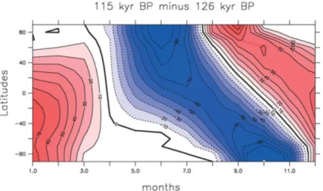
Fig. 1. Insolation change at the top of the atmosphere (in Wm-2), differences between 115 kyr BP, corresponding to the inception, and 126 kyr BP, corresponding to the optimum interglacial. Contour in-tervals are every 10 Wm-2.
Fig. 1. Changement d’insolation au sommet de l’atmosphère entre 115 ka, correspondant à la transition interglaciaire/glaciaire, et 126 ka, correspondant à l’optimum interglacière.
2.1. A series of failures
The simple argument of Milankovitch’s theory[28]
is that the decreased summer insolation at the northern hemisphere’s high latitudes would produce a sufficient cooling for inhibiting the melting of the snow fallen during the winter season (Fig. 1). The difference in albedo then produces a positive feedback that can trig-ger large ice sheets’ extension. Very early in the 1980s, such ideas have been quantified by Atmospheric Gen-eral Circulation Models (AGCM). The test was very simple and consisted in modifying the orbital parame-ters to account for changes in insolation at the top of the atmosphere[1]and to analyse the response of the climate system (i.e. the atmosphere) in terms of cool-ing and snowfall distributions. All the experiments that tried to test Milankovitch’s theory with AGCM found that it was impossible to produce perennial snow in re-gions where Fennoscandian and Laurentide ice sheets started to expand[31,32].
During the last decade, with a major increase in palaeoclimatic reconstruction and modelling studies, it appears that these failures were due to two ma-jor weaknesses. First, whereas the atmospheric model amplified the cooling due to reduced summer insola-tion, it was still far to become cold enough to prevent snow from melting. Second, because of the cooling, the wintertime atmosphere was also drier, therefore preventing any increase in snowfall rate. In the 1990s,
the idea developed that the sensitivity of the model was too weak, because some important components of the climate system were missing, like the vegetation and the ocean. In a subsequent set of experiments, it has been shown that taking into account the changes in vegetation produced by a colder climate helped to amplify the initial simulated cooling. In response to the atmospheric model cooling, there is a south-ward progression of areas covered by Tundra (short and scattered type of vegetation) in northern high-latitude lands at the expense of boreal forests[8,15]. This sole change amplified the high-latitude albedo and increased the length of the season of snow-covered lands. Nevertheless, even if the biosphere plays an im-portant role and increases the duration of the snow cover, this feedback remains too weak to lead to peren-nial snow cover.
2.2. The water cycle and the role of the ocean Indeed, the second important component, which was missing in these simulations, is the ocean. The first simulations using AGCM assessed that the sea-surface temperatures (SSTs) at the end of Last Inter-glacial, were very similar to present-day ones, a state-ment, in the light of recent SSTs reconstruction for this period, that turned out to be false[7]. A first at-tempt to account for insolation changes on SSTs was performed by Dong and Valdes[9], who coupled the UGAMP AGCM to a slab-ocean model. This study shows that indeed the ocean reacts to changes in in-solation, but the response appears to be too large com-pared to the data[6,7]. Moreover, such a slab ocean is only able to depict the thermal response of the 50-m mixed layer and does not account at all for changes in ocean dynamics. The next step was therefore to use an atmosphere–ocean general circulation model. This step became possible at the beginning of this century, when coupled ocean–atmosphere models were able not only to produce reliable results over continents and oceans, but also when they were able to predict a good sea–ice seasonal cycle, which is a key feature to cope with the inception period. More recently, Meiss-ner et al. [27] showed that only a synergy of ocean atmospheric and vegetation allows producing the on-set of ice sheets.
A coupled OAGCM simulation has been performed using IPSL OAGCM and the results can now be
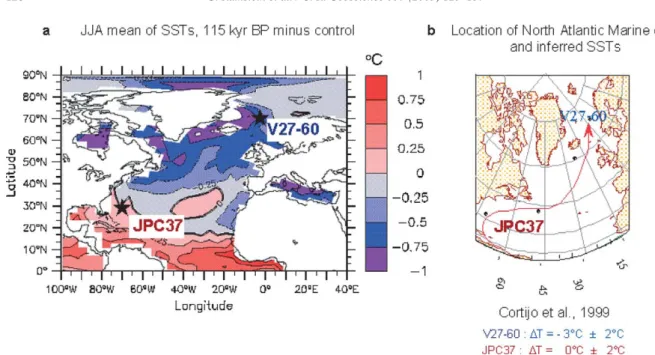
di-Fig. 2. Model-data comparison for SST in the North Atlantic Ocean. (a) Sea-surface temperature (SST) calculated by the IPSL coupled model for the last glacial inception climate (in Celsius) with respect to the simulated present-day climate (control). (b) Location of V27-60 and CH69-K9 marine cores in the North Atlantic Ocean and inferred SST shown with respect to the present-day one. The red arrow traces the main pathway of present-day North Atlantic drift.
Fig. 2. Comparaison des résultats de modèles pour les températures de surface de l’Atlantique nord. (a) Température de surface de l’océan (SST) calculée par le modèle OAGCM de l’IPSL entre 115 ka BP et le présent. (b) SST reconstruites à partir des carottes marines de l’Atlantique nord V 27-60 et CH69-K9, entre 115 ka et le présent. Les tirets rouges représentent la dérive nord-atlantique actuelle.
rectly compared with SSTs inferred from marine cores
[22]. The comparison between model results and SSTs reconstructions in the North Atlantic, which is the key region for this study, is shown inFig. 2. The remark-able feature is that the geographical pattern is very well reproduced: a cooling over the high latitudes of North Atlantic, whereas the tropical North Atlantic is warmer or similar to present-day temperatures. As we will discuss later, this feature is very important to understand the impact of the water cycle on climate.
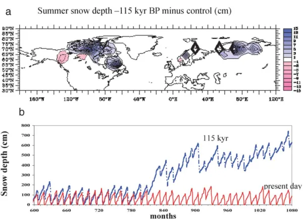
Fig. 3a shows that the summer snow depth increases over regions where it is believed that ice sheets began to grow. After several years, for a grid point corre-sponding to the Canadian Archipelago, the 115-kyr-BP simulation is able to produce perennial snow cover and then snow accumulation[22](seeFig. 3b). In this study, it has been shown that superimposed on an in-crease of about 3% of the northward atmospheric heat transport, there is also a decrease, of about 6%, of the northward ocean heat transport. The location of the deepwater formation is shifted to lower latitudes, due to the increased sea ice extension, whereas the depth
of the North Atlantic Deep Water is reduced by about 1000 m.
On the other hand, the amplified North Atlantic SSTs gradient due to the insolation changes induces a larger northward atmospheric moisture transport from the warmer tropical ocean and provides by this way an excess of moisture availability for high latitudes. In this coupled experiment, the simulated water cycle changes have three major impacts over the high lati-tudes climate:
(i) the annual mean increase of water runoff into the Arctic Ocean induces an extension and deepen-ing of the halocline, which, associated to cooler surface water, allows a progression of Arctic sea ice volume and extension. This change in sea ice characteristics contributes to enhance the cooling of surrounding lands, like the Cana-dian Archipelago, because of the increased local albedo;
(ii) the increase of freshwater input into the Arc-tic Ocean induces a reduction of the sea surface
Fig. 3. (a) Increased summer snow depth (in cm) over North America and northern Europe simulated by the IPSL model for the last glacial inception with respect to the present-day climate. The values are scaled between±15 cm with a 2-cm interval. The blue (red) shading indicates an increase (decrease). (b) Snow accumulation over the Canadian Archipelago during the present-day simulation (red curve) and simulation at 115 kyr (blue curve). Each year, the summer snow depth decreases to zero in the control run, whereas, in the simulation at 115 kyr BP, there is clearly a large accumulation of snow and a perennial cover.
Fig. 3. (a) Épaisseur de neige estivale (cm) au-dessus de l’Amérique du Nord et de l’Europe, simulée par le modèle de l’IPSL pour l’entrée en glaciation par rapport à l’Actuel. Les valeurs s’étalent entre±15 cm, avec un intervalle de 2 cm. La couleur bleue indique une augmentation, le rouge une diminution. (b) Accumulation de neige sur l’Archipel canadien pour l’Actuel (en rouge) et pour 115 ka (en bleu). On constate que la neige ne s’accumule pas à l’Actuel et fond totalement en été, tandis qu’on observe, à 115 ka, de la neige pérenne et une forte accumulation.
salinity. The subsequent reduced meridional den-sity gradient in the northern seas leads to a shift of deepwater formation location toward lower lat-itudes, which, in turn, inhibits the possibility of bringing heat by ocean dynamics toward high lat-itudes;
(iii) finally, because of the amplified high latitudes cooling by both feedbacks described herein (points 1 and 2), the increase in water transport towards high latitudes is translated into increased snowfall over regions where ice sheets will grow. The major advance of this study compared to previ-ous experiments was to show that, before accumulat-ing snow and therefore triggeraccumulat-ing the ‘Milankovitch’
effect, it is necessary to provide more moisture in northern high latitudes. These changes in the water cy-cle will amplify the high latitudes cooling due initially to the insolation changes through an intricate network of feedbacks – involving sea ice and ocean –, but will also moist the atmosphere where snow delivery has to increase. All these reasons make the water cycle an important contributor to the shift from interglacial to glacial states all along glacial cycles of the Quaternary.
3. The origin of the Indian Monsoon
The second example illustrating the role of the wa-ter cycle in climate change concerns the origin of the
Indian monsoon. Many studies[24–26]invoke the fact that, during the Late Tertiary, the uplift of the Tibetan Plateau and Himalaya plays a major role in the devel-opment of the Indian monsoon. The main feature of the present-day monsoon is obviously the heavy sum-mer rainfalls over southeastern Asia. These rainfalls are the result of a huge moisture advection driven by the Indian Ocean–Eurasian continent thermal gradient. A change in the Indian Ocean–Eurasia thermal gradi-ent should consequgradi-ently modify the Asian monsoon. Thus, at geological timescales, plate tectonics should be able to modulate the intensity and location of the Asian monsoon.
Kutzbach et al.[24–26]proposed that the uplift of the Himalaya mountain range as well as of the Tibetan plateau in response to the India–Asia collision has driven the onset of Indian monsoon. The height of the Tibetan plateau and Himalaya appears to be a key for-cing factor in the development of the Asian monsoon. They showed, using an AGCM, that the uplift of the Tibetan plateau enhanced the summer monsoon pre-cipitation over southeastern Asia. These experiments were limited by two major aspects:
– the coarse spatial resolution of the AGCM used in their study does not allow for the representation of the Himalaya mountain ranges; the Himalayan and the Tibetan plateau are represented by a single geological structure;
– their study consisted in three crude sensitivity ex-periments to the height of the Tibetan plateau. In a first step, the whole plateau is lowered to 400 m (no plateau experiment), then the present-day ele-vation of the Tibetan plateau is reduced by a half (half-elevation experiment), and at last, they sim-ulate the climate using the present day topography (full elevation experiment).
Although the AGCM was forced using a crude palaeogeography, they clearly show that the intensity of the Asian summer monsoon is a function of the ele-vation of the Tibetan plateau.
The palaeogeographical context evolved drastically over the past 30 Myr in Eurasia (Fig. 4). The major striking features are:
(i) the rise of the Tibetan plateau and of the Hi-malayas chain. Although the India-Asia collision
is at the origin of these uplifts, the evolution of these two geological objects is different;
(ii) the lateral extrusion of Indochina as a conse-quence of the India-Asia collision;
(iii) the progressive shrinkage of the Paratethys Sea, which covers the eastern part of Europe and a large part of Siberia and Central Asia, in response to the large-scale deformation of the southern margin of Eurasia.
We used the LMD AGCM numerical model to simulate the climate corresponding to these two dif-ferent periods: 30 Myr ago, a situation where the Paratethys is large and for which there is no uplift; and 10 Myr ago, a situation where the Paratethys has already shrunk, while the plateau uplift is already im-portant.
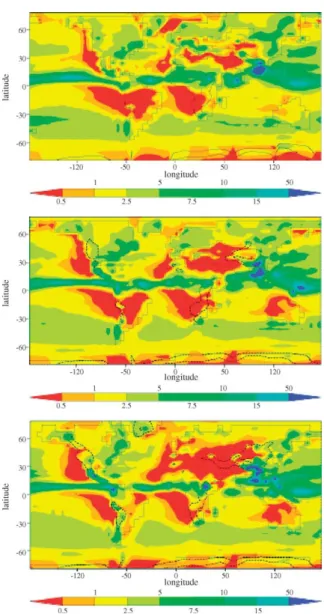
In a first step, we performed experiments with the most realistic palaeogeography for 30 and 10 Myr[14, 29]. Forcing the AGCM with a set of boundary condi-tions representing the major features of the Oligocene period, we showed that a monsoon circulation produ-cing rainfall mainly over Indochina existed prior to the main uplift of the Tibetan Plateau and the Himalaya (Fig. 5).
The change in palaeogeography enhanced the sum-mer thermal gradient, increasing the moisture advec-tion over southern Asia, inducing heavy rainfalls dur-ing the summer. However, the change in monsoon is not only due to a change in the thermal gradient. The atmospheric circulation is also deeply altered. The intensity and direction of winds are changed, brin-ging more and more moisture towards the Himalaya chain in the two last experiments, at 10 Myr and nowadays. The rise of moist air masses along the Hi-malayan southern flank generates heavy rainfalls over this mountain range (Fig. 5), enhancing the mechani-cal erosion of the Himalaya[14,26].
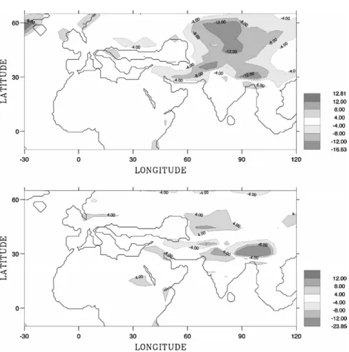
The thermal evolution of the Asian continent from a seasonal point of view clearly appears to be a key characteristic for the monsoon evolution. InFig. 6, we show the winter and summer air temperature differ-ences between 30 and 10 Myr. As we could expect, the shrinkage of the Paratethys (i.e. the fact that an epi-continental sea disappears) has for consequences the warming of the Eurasian continent during the sum-mer season and its cooling during the winter season (Fig. 6).
Fig. 4. Palaeogeography at 30 Myr (top), at 10 Myr (middle) and at the present day (bottom) used as boundary conditions[3,4]. The main changes are the uplifts of the Himalayas and of the Tibetan plateau, and the progressive retreat of an epicontinental sea in Eurasia, the Paratethys Sea. The Middle East emerged during the Early Miocene, as well as the lateral extrusion of Indochina, in response to the India–Eurasia convergence. White areas represent oceans and seas.
Fig. 4. Paléogéographies à 30 Ma (haut), 10 Ma (milieu) et actuelle (bas), utilisées comme conditions aux limites des simulations avec LMDZ. Les principaux changements sont la surrection du plateau tibétain et de la chaîne Himalayenne, ainsi que le retrait progressif de la mer épi-continentale Paratéthys. Le Moyen Orient émerge dès le début du Miocène, ainsi que l’extrusion latérale de l’Indochine liée à la convergence Inde–Asie.
Fig. 5. Simulated summer precipitation (mm d−1) at 30 Ma (top), at 10 Ma (middle) and at PD (bottom).
Fig. 5. Précipitations d’été simulées (mm j−1) à 30 Ma (haut), à 10 Ma (milieu) et à l’Actuel (bas).
Moreover, it is possible with a GCM to quantify the separate impact of the uplift of the Tibetan Plateau and Himalayas and that of the shrinkage of the Paratethys. We therefore performed two more experiments: one without uplift and a second without shrinkage.
In fact, these simulations[14,29]showed that the plate tectonics modulates the distribution and inten-sity of the Asian monsoon at the geological time scale, but that the monsoon over southeastern India did
ex-ist already during the Oligocene or Early Miocene[5, 13,20]. Both the uplift and the shrinkage act on the summer thermal gradient between Asia and the In-dian Ocean, and modify the atmospheric circulation and moisture advection to modulate the summer geo-graphical pattern of monsoon.
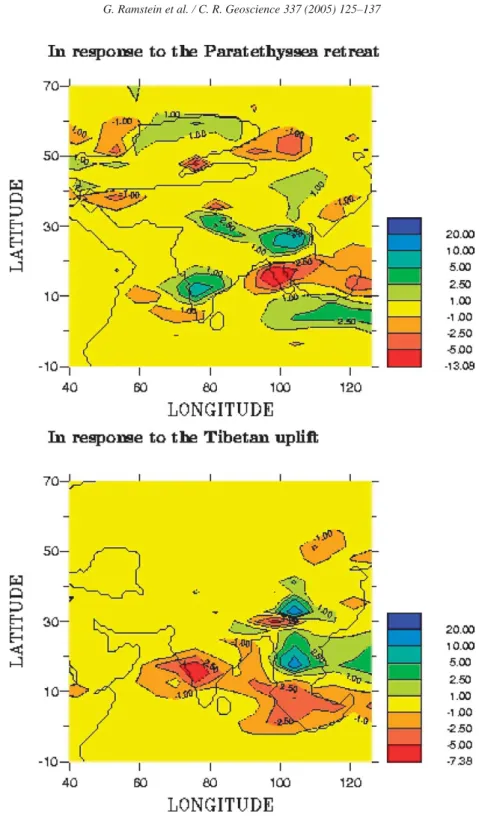
As shown inFig. 7, the difference on rainfall due to the plateau uplift is nevertheless much more lo-cal (linked to the orogenesis), whereas the shrinkage of the epicontinental sea has a broader and more re-gional effect. The redistribution of monsoon rainfall is largely driven by palaeogeographic evolution at this timescale.
4. Glaciations of the Neoproterozoic 4.1. Snowball hypothesis
The Earth’s history is surprising. Due to a fainter sun (the insolation at the top of the Earth’s Atmosphere has increased from 80% to the present-day value dur-ing the last 2 Gyr), the surface of the Earth should have been covered with ice. Such a result has been simu-lated with a simple Energy Balance Model[2].
But to get out of a snow-covered Earth, the so-called ‘snowball Earth’, an enormous quantity of en-ergy is necessary due to the obviously very large albedo. Indeed, the albedo of a snowball Earth is around 0.7, whereas the present-day albedo is around 0.3. Therefore, in a snowball Earth context, most of the incoming solar radiation is reflected. This feature explains the difficulty to initiate deglaciation from an Earth totally covered with ice. This paradigm lasted for more than 20 years, until Kirschvink[24]argued that a very important component was missing in the Budyko scenario (only accounting for albedo changes in an EBM model): the carbon cycle.
Indeed, if the Earth were totally covered with ice sheets over continents and sea-ice over oceans, the water cycle would be seriously damped by a fac-tor form 10 to 100, depending on the simulations
[4,12]. Most importantly, the sink of carbon at geo-logical timescales (the continental weathering) shuts off, while the source of carbon (the outgassing through volcanoes and the mid-oceanic ridge) keeps on injec-ting CO2in the atmosphere, where it accumulates for
Fig. 6. Temperature difference (◦C) in winter (top) and summer (bottom) between the experiment at 10 Myr and that at 30 Myr. Dashed (continuous) lines represent isotherms below (above) 0◦C.
Fig. 6. Différence de température d’hiver (haut) et d’été (bas) entre les simulations à 10 et 30 Ma. Les lignes pointillées (continues) représentent les isothermes au-dessous (au-dessus) de zéro.
reaches a threshold value estimated to be 0.12 bar[3], a huge deglaciation occurs and produces the so-called cap-carbonates seen everywhere above the Neopro-terozoic glacial sediments. Such a scenario may also explain the reappearance of the banded iron forma-tions (BIF), which have disappeared since 2.4 Gyr and were due to global anoxia in the ocean.
These scenarios led a lot of climate modellers to quantitatively test these ideas of a large or full glacia-tion during the Neoproterozoic. Many GCM mod-els and simulations with more simple modmod-els[11,21]
show that it was possible to simulate a snowball Earth in the Neoproterozoic context (i.e., accounting for palaeogeography, weaker insolation by 6%, and rather low value of CO2). The results of the IPSL LMDz
OAGCM coupled with a swamp model for Sturtian palaeogeography are presented.
The fact that the reduction of the solar constant is large enough to produce a global glaciation in our nu-merical simulations is in reality facilitated by the low atmospheric CO2level, which cannot compensate for
the deficit of solar energy due to the faint young Sun. 4.2. Carbon cycle
Most of the obtained results strongly depend on the prescribed atmospheric CO2 level in these
sim-ulations. There is indeed no way to infer from any proxy the value of atmospheric CO2 during these
Fig. 7. Sensitivity experiments to the Tibetan Plateau and Himalayas’ uplifts (top) and to the Paratethys shrinkage (bottom). The impact of the uplift on summer precipitation is more local than the impact of the Paratethys shrinkage.
Fig. 7. Expériences de sensibilité à la surrection du plateau tibétain et de la chaîne himalayenne (haut) et au retrait de la Paratéthys (bas). L’impact de la surrection sur les précipitations est plus local que celui du retrait de la Paratéthys.
between climate and carbon cycle is to use a carbon– climate model adapted for geological timescales. To achieve this goal, the model of intermediate complex-ity, CLIMBER-2, [16,17], has been coupled to the COMBINE model, which calculates the main features of C, P, and O biogeochemical cycles[19].
The most difficult challenge is to explain why the CO2 should have strongly decreased and
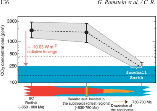
there-fore triggered the onset of a global glaciation. Us-ing our new model, called GEOCLIM (for GEO-logical timescales CLImate Model), we have shown that tectonics plays a major role during the Neopro-terozoic[10,30]. The dispersal of the Rodinia super-continent results in an enhanced consumption of at-mospheric CO2, decreasing from a pCO2of 1830 ppm
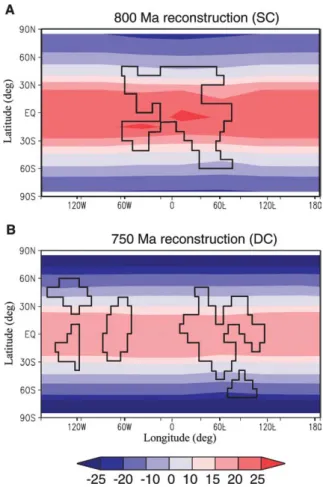
to 510 ppm, i.e. consumption in the order of 1320 ppm. This is due to the larger runoff occurring over the equatorial regions presenting a dispersed configura-tion, which triggers larger weathering rates, and a sig-nificant global cooling of ∼ 8◦C (Fig. 8). We have further demonstrated that experiments accounting for the palaeogeographic impact on weathering rates to-gether with the weathering of the large magmatic provinces produce conditions appropriate to trigger a full snowball glaciation at 750 Ma (Fig. 9). Indeed, the break-up of the Rodinia supercontinent is heralded by and accompanied with the eruptions of large basaltic provinces[27], resulting in an increase of the weather-ability of the continental surface and consumption of atmospheric CO2over the long timescale[18].
These studies provide support for the fact that the modification of the water cycle in response to the shift of continental plates may have been responsible for a long-term atmospheric CO2 decrease. The efficiency
of the proposed mechanism relies on the tropical po-sition of the continents at this time. Indeed, the wa-ter cycle is very efficient over this region. The in-crease in runoff is able to produce a huge consumption of atmospheric CO2 via the continental weathering
processes.
5. Conclusion
These three very different contexts illustrate the role of the water cycle in Earth’s Climate history at various timescales. From clouds to sea ice and from ice sheets build-up to thermohaline circulation, water
Fig. 8. Annual mean surface air temperature (◦C) simulated by the CLIMBER-2 model. (A) With a pCO2 of 1830 ppm and for the
continental reconstruction at around 800 Myr[30,31](noted SC as Supercontinent Configuration), i.e. prior to the Rodinia break-up. (B) With a pCO2of 510 ppm and for the continental
reconstruc-tion at around 750 Myr[32](noted DC as Dispersed Configura-tion). Boundary conditions include a solar luminosity 6% below the present-day value. In addition, we assume that the Earth’s orbit around the Sun was circular (eccentricity= 0) and that the Earth’s obliquity was 23.5◦. This setting leads to an equal annual insolation for both hemispheres. The land surface in the climate model has the radiative characteristics of a desert and has a uniform elevation of 100 m for both palaeogeographies.
Fig. 8. Moyenne annuelle des températures de surface simulées par le modèle CLIMBER-2. (A) avec pCO2= 1830 ppm, et
reconstruc-tion continentale correspondant à 800 Ma[30,31](notée SC, su-percontinents antérieurs au break-up) ; (B) avec pCO2= 510 ppm,
avec une configuration des continents correspondant à 750 Ma[32]
(noté DC, continents dispersés). Les deux expériences sont effec-tuées avec une baisse de l’insolation au sommet de l’atmosphère de 6 %, par rapport à la valeur actuelle. L’excentricité de l’orbite est nulle et l’obliquité de 23,5◦. Le relief a une élévation de 100 m, pour les deux paléogéographies.
Fig. 9. Steady-state atmospheric CO2level achieved by GEOCLIM
(1) for the SC runs, (2) for the SC runs with the inclusion of basaltic provinces, and (3) for the DC runs also with basaltic provinces. Ver-tical bars denote the upper and the lower range of atmospheric CO2
levels, calculated using (1) a 20% increase and a 20% decrease in degassing flux for the SC runs, (2–3) a 20% increase and a basaltic surface of 4× 10⁶km2, and a 20% decrease and a basaltic surface of 8× 10⁶km2for the SCtrap and DCtrap runs.
Fig. 9. Niveau à l’équilibre de CO2atmosphérique calculé par
GEO-CLIM (1) pour la simulation « SC », (2) pour la simulation « SC trap » incluant les basaltes, (3) pour la simulation « DC trap » in-cluant également les basaltes. L’enveloppe représente les niveaux de CO2atmosphérique maximum et minimum calculés par le
mo-dèle (1) pour des valeurs du dégazage augmentées et/ou diminuées de 20 % par rapport à sa valeur actuelle (2–3) pour une valeur du dé-gazage augmentée de 20 % et une surface basaltique de 4×10⁶km2 et pour une valeur de dégazage diminuée de 20 % et une surface ba-saltique de 8× 10⁶km2, et ce pour les runs « SC trap » et « DC trap ».
is one of the key components of the Earth System. Many processes are very short (clouds physics), but others explain climate changes at Myr scales (weath-ering and CO2burial).
What has been shown for the Earth’s history is also true for the future climate of our planet.
The climate of the beginning of this century should be dominated by the impact of greenhouse gases (and water is one of these gases). With increasing temper-ature, the capability of atmosphere to contain water vapour will also increase and this is a positive feed-back, which in turn will lead to increase again the temperature. This scenario has to be modulated be-cause of cloud changes that may have positive (high clouds) or negative (low clouds) feedbacks.
Obviously, the sea level will rise with the glaciers disappearance, but, more importantly, the problem may come from the destabilisation of the ice sheets (Greenland and Antarctica). How fast may this
oc-cur? Which meltwater amount does it induce? How may Global Climate and thermohaline circulation be affected? Models that have been tested on past climate changes may be helpful to try to give a quantified an-swer to these questions.
References
[1] A.L. Berger, Long-term variations of daily insolation and Qua-ternary climatic changes, J. Atmos. Sci. 35 (1978) 2362–2367. [2] M.I. Budiko, The effect of solar radiation variations on the
cli-mate of the Earth, Tellus 21 (1969) 611–619.
[3] K. Caldeira, J.F. Kasting, Susceptibility of the early Earth to irreversible glaciation caused by carbon dioxide clouds, Na-ture 359 (1992) 226–228.
[4] M.A. Chandler, L.E. Sohl, Climate forcings and the initiation of low-latitude ice sheets during the Neoproterozoic Varanger glacial interval, J. Geophys. Res. 105 (2000) 20737–20756. [5] G. Chenggao, R.W. Renaut, The effect of Tibetan uplift on the
formation and preservation of Tertiary lacustrine source-rocks in eastern China, J. Paleolimnol. 11 (1994) 31–40.
[6] E. Cortijo, et al., Eemian cooling in the Norwegian Sea and North Atlantic ocean preceding continental ice-sheet growth, Nature 372 (1994) 446–449.
[7] E. Cortijo, S. Lehman, L. Keigwin, M. Chapman, D. Paillard, L. Labeyrie, Changes in meridional temperature and salinity gradients in the North Atlantic Ocean (308–728N) during the Last Interglacial Period, Paleoceanography 14 (1999) 23–33. [8] N. de Noblet, C. Prentice, S. Joussaume, D. Texier, A. Botta, A.
Haxeltine, Possible role of atmosphere–biosphere interactions in triggering the last glaciation, Geophys. Res. Lett. 23 (1996) 3191–3194.
[9] B.W. Dong, P.J. Valdes, Sensitivity studies of northern hemi-sphere glaciation using an atmospheric general circulation model, J. Climate 8 (1995) 2471–2496.
[10] Y. Donnadieu, Y. Goddéris, G. Ramstein, A. Nédélec, J. Meert, A ‘snowball Earth’ climate triggered by continental break-up through changes in runoff, Nature 428 (2004) 303–306. [11] Y. Donnadieu, G. Ramstein, F. Fluteau, D. Roche, A.
Ganopol-ski, The impact of atmospheric and oceanic heat transports on the sea ice-albedo instability during the Neoproterozoic, Clim. Dyn. 22 (2004) 293–306.
[12] Y. Donnadieu, F. Fluteau, G. Ramstein, C. Ritz, J. Besse, Is there a conflict between the Neoproterozoic glacial deposits and the snowball Earth model: an improved understanding with numerical modelings, Earth Planet. Sci. Lett. 208 (2003) 101– 112.
[13] S. Ducrocq, Y. Chaimanee, V. Suteethorn, J.-J. Jaeger, Ages and paleoenvironment of Miocene mammalian faunas from Thailand, Palaeogeogr. Palaoeclimatol. Palaeoecol. 108 (1994) 149–163.
[14] F. Fluteau, G. Ramstein, J. Besse, Simulating the evolution of the Asian and African monsoons during the past 30 millions years using an atmospheric general circulation model, J. Geo-phys. Res. 104 (1999) 11995–12018.
[15] R.G. Gallimore, J.E. Kutzbach, Role of orbitally-induced vege-tative changes on incipient glaciation, Nature 381 (1996) 503– 505.
[16] A. Ganopolski, C. Kubatzki, M. Claussen, V. Brovkin, V. Petoukhov, The influence of vegetation–atmosphere–ocean interaction on climate during mid-Holocene, Science 280 (1998) 1916–1919.
[17] A. Ganopolski, S. Rahmstorf, V. Petoukhov, M. Claussen, Sim-ulation of modern and glacial climates with a coupled model of intermediate complexity, Nature 391 (1998) 351–356. [18] Y. Goddéris, Y. Donnadieu, A. Nédelec, B. Dupré, C. Dessert,
A. Grard, G. Ramstein, L.M. François, The Sturtian ‘snowball’ glaciation: fire and ice, Earth Planet. Sci. Lett. 211 (2003) 1– 12.
[19] Y. Goddéris, M.M. Joachimski, Global change in the Late De-vonian: modelling the Frasnian-Famennian short-term carbon isotope excursions, Palaeogeogr. Palaeoclimatol. Palaeoecol-ogy 202 (2003) 309–329.
[20] Z.T.Y. Guo, W.F. Ruddiman, Q.Z. Hao, H.B. Wu, Y.S. Qiao, R.X. Zhu, S.Z. Peng, J.J. Wei, B.Y. Yuan, T.S. Liu, Onset of Asian desertification by 22 Myr ago inferred from loess de-posits in China, Nature 416 (2002) 159–163.
[21] W.T. Hyde, T.J. Crowley, S.K. Baum, R.W. Peltier, Neo-proterozoic ‘snowball Earth’ simulations with a coupled climate/ice-sheet model, Nature 405 (2000) 425–429. [22] M. Khodri, Y. Leclainche, G. Ramstein, P. Braconnot,
O. Marti, E. Cortijo, Simulating the amplification of orbital forcing by ocean feedbacks in the last glaciation, Nature 410 (2001) 570–574.
[23] M. Khodri, G. Ramstein, N. de Noblet-Ducoudre, M. Ka-geyama, Sensitivity of the northern extratropics hydrological cycle to the changing insolation forcing at 126 and 115 kyr BP, Clim. Dyn. 21 (2003) 273–287.
[24] J.E. Kutzbach, P.J. Guetter, W.F. Ruddiman, W.L. Prell, Sen-sitivity of climatic uplift in southern Asia and in the
Ameri-can West: Numerical experiments, J. Geophys. Res. 94 (1989) 18393–18407.
[25] J.E. Kutzbach, W.L. Prell, W.F. Ruddiman, Sensitivity of Eurasian climate to surface uplift of Tibetan plateau, J. Geol. 101 (1993) 177–190.
[26] J.E. Kutzbach, W.F. Ruddiman, W.L. Prell, Possible effects of Cenozoic uplift and CO2lowering on global and regional
hy-drology, in: W.F. Ruddiman (Ed.), Tectonic Uplift and Climate Change, Plenum Press, New York, 1997, pp. 149–170. [27] K.J. Meissner, A.J. Weaver, H.D. Matthews, P.M. Cox, The
role of land surface dynamics in glacial inception: a study with the UVic Earth System Model, Clim. Dyn. 21 (2003) 515–537. [28] M.K. Milankovitch, Kanon der Erdbestrahlung und seine An-wendung auf das Eiszeitenproblem, Serb. Acad. Beorg. Spec. Publ. 132 (1941) (in German); Canon of insolation and the Ice Age problem (Israel Program for Scientific Translation, Jerusalem, 1969) (English translation).
[29] G. Ramstein, F. Fluteau, J. Besse, S. Joussaume, Effect of orogeny, plate motion and land-sea distribution on Eurasian climate over the past 30 million years, Nature 386 (1997) 788– 795.
[30] G. Ramstein, Y. Donnadieu, Y. Godderis, Les glaciations du Protérozoïque, C. R. Geoscience 336 (2004) 639–646. [31] D. Rind, D. Peteet, G. Kukla, Can Milankovitch orbital
varia-tions initiate the growth of ice sheets in a general circulation model?, J. Geophys. Res. 94 (1989) 12851–12871.
[32] J.-F. Royer, M. Déqué, J.-R. Petit, A sensitivity experiment to astronomical forcing with a spectral GCM: simulation of the annual cycle at 125 000 BP and 115 000 BP, in: A.L. Berger, J. Imbrie, J. Hays, G. Kukla, B. Saltzman (Eds.), Milankovitch and Climate, vol. 2, D. Reidel, Dordrecht, the Netherlands, 1984.
![Fig. 4. Palaeogeography at 30 Myr (top), at 10 Myr (middle) and at the present day (bottom) used as boundary conditions [3,4]](https://thumb-eu.123doks.com/thumbv2/123doknet/2339816.33643/8.892.177.727.206.922/fig-palaeogeography-myr-myr-middle-present-boundary-conditions.webp)