Improvement of Biogenic Carbon Accounting in the Life Cycle of Wood used in Construction in Canada

(1)

POLYTECHNIQUE MONTRÉAL

affiliée à l’Université de Montréal

Improvement of Biogenic Carbon Accounting in the Life Cycle of Wood used

in Construction in Canada

MARIEKE HEAD

Département de mathématiques et de génie industriel

Thèse présentée en vue de l’obtention du diplôme de Philosophiae Doctor Génie industriel

Septembre 2019

(2)

POLYTECHNIQUE MONTRÉAL

affiliée à l’Université de Montréal

Cette thèse intitulée:

Improvement of Biogenic Carbon Accounting in the Life Cycle of Wood used

in Construction in Canada

présentée par Marieke HEAD

en vue de l’obtention du diplôme de Philosophiæ Doctor a été dûment acceptée par le jury d’examen constitué de :

Louis FRADETTE, PhD, président

Manuele MARGNI, PhD, membre et directeur de recherche Annie LEVASSEUR, PhD, membre et codirectrice de recherche Robert BEAUREGARD, PhD, membre et codirecteur de recherche Cécile BULLE, PhD, membre

(3)

DEDICATION

For Amelia and Lentil,

“Wat geweldig dat niemand ook maar één moment hoeft te wachten met het verbeteren van de wereld.” (“How wonderful it is that nobody need wait a single moment before starting to improve the world.”) Anne Frank

“We must reinvent a future free of blinders so that we can choose from real options.” David Suzuki

(4)

ACKNOWLEDGEMENTS

The end of the road! I sometimes never thought that this moment would actually happen!

First, a big thank you to my supervisors. To Manuele, thank you for allowing me a great degree of independence in my work, while still giving me thorough feedback and insights on my work and having me take a step back to see the bigger picture of what my work contributes. To Annie, thank you for being such a wonderful sounding board and for our deep methodological discussions. To Robert, thank you for sharing your wealth of knowledge on forestry science and for your expansive professional network that allowed me the opportunity to collaborate with forestry scientists. During my PhD, I also had the opportunity for some enriching collaborations. Thank you to the Pacific Forestry Centre (PFC) in Victoria, British Columbia for hosting me in August 2016. Thank you to Werner Kurz for your helpful insights in our discussions and for your support in my learning of CBM-FHWP and for having welcomed me into the carbon team. A big thanks to Michael Magnan, you were invaluable and ever so patient in teaching me how to use CBM-FHWP and supporting the modelling that I was carrying out. I really appreciate your kindness in making sure that I felt at home at PFC and in Victoria. Finally, thanks to Pierre Bernier for his collaboration on my first article and your extra support and patience in helping me understand forestry science. To everyone at CIRAIG over the years, thank you for providing such a friendly and welcoming research environment. In particular, thanks to the following people (in alphabetical order). To Anders, for your humour and all of the interesting conversations that ranged from work to our mutual love of Radiohead. To Andrea, for our discussions of all things vegan. To Anne-France, for simultaneously interesting but hilarious conversations. To Breno, for your support both as a fellow PhD student and as a friend. To Catherine, for our conversations and mutual support over the years. To Charles, for always regularly keeping in touch, and your friendship and work collaborations beyond CIRAIG. To Gabrielle, for our interesting conversations as office mates. To Gaël, for our bantering discussions. To Hassana, for your enthusiasm. To Ivan for always being so uplifting. To Julien P, for your friendliness and ability to have a conversation about anything. To Laure, for your positive energy in our office. To Rifat, for your smiles and support. To Sara, for our summer runs over Mont Royal over the years. To Wafaa, for our conversations about kids and life as PhD moms. Also, thanks to everyone else I may not have mentioned specifically!

(5)

To my Montreal friends, thanks for your friendship over the years and being a very needed distraction from my PhD. Thanks to the following people. To Tara, for your relentless enthusiasm and our ability to have never ending conversations. To Kim, for our awesome bike rides and potluck chats over the years. To Annelies, for being such a kind friend during your time in Montreal. To Abilash and Annabelle, for your enthusiasm and friendship. To Line, for being such a great friend over the years and our fun times playing board games, canning, watching complicated Iceland TV series with a crying baby, snowshoeing and bike touring. To Jin, for our mom chats and mutual support club. To our neighbours, especially Miryam, Isaac, Lyne, Sylvain, and Valentina. You’ve been the most generous and friendly neighbours we could have asked for. Rachel for always being there, for being one of the most generous people I know, for our lunches, swim meet ups, brunches, bike rides, etc.

To my family. First, a big thanks to my parents for your unwavering support over the years and your willingness to come and travel to New Hampshire to watch Amelia while I attended a conference and more recently your support through some tough times. To Lucy, for keeping me company in the home stretch of my PhD and for forcing me out for daily walks even in the coldest and rainiest weather. To Amelia, you’ve lived and breathed this thesis too from the time you kept me company in Victoria while you were still on the inside to the hilarious little toddler that you’ve become. To Lentil, though you’re not with us anymore, you leaving this world helped me build strength and resilience in finishing this PhD. And finally, to Anthony, you’re my rock, my world, my everything, and I couldn’t have done this without your encouragement, your “papadag” in Amelia’s first year so that I could continue my work, for your support and help with some coding work, and especially for supporting me immensely in these last few difficult months. I love you so much!

(6)

RÉSUMÉ

Au Canada, le bois est généralement utilisé comme matériau de construction. Cependant, il existe des limites dans la méthodologie de comptabilité des impacts climatiques des matériaux de construction en bois en analyse de cycle de vie (ACV). Typiquement, en ACV, l’hypothèse de la neutralité du carbone biogénique est utilisée pour la biomasse et pour les produits issus du bois, puisque le carbone séquestré par la biomasse est égal au carbone qui est émis éventuellement par cette biomasse en fin de vie. Étant donné la nature dynamique des émissions de dioxyde de carbone et de l’effet de serre, le paradigme simpliste qu’un bilan de carbone neutre est égal à la neutralité de carbone est remis en question.

Il y a une quantité croissante de preuves scientifiques indiquant que les impacts climatiques réels des produits issus du bois dépendent de plusieurs facteurs, dont le temps de stockage et le timing des émissions, le type d’aménagement forestier et le type de traitement en fin de vie. L’objectif global de ce travail doctoral est de développer une méthode qui comptabilise systématiquement la captation, l’émission et le stockage de carbone biogénique dans les ACV du bois utilisé dans les bâtiments en 1) développant des profils de flux de carbone qui sont différentiés temporellement en tenant compte de la dynamique du carbone forestier, 2) développant des profils de flux de carbone différentiés temporellement du point de récolte jusqu’à la fin de vie, et 3) mettant en pratique l’ACV dynamique aux profils de flux de carbone différentiés temporellement pour une ACV berceau-au-tombeau d’un produit issu de bois.

La plupart des ACV ne considèrent pas l’aménagement forestier des produits issus du bois. Ce travail de recherche vise à améliorer la comptabilité du carbone biogénique de la phase forestière du cycle de vie des produits issus de bois au Canada. Ceci implique la modélisation spécifique des flux de carbone en fonction des espèces d’arbres, des conditions de croissance et des pratiques d’aménagement forestier des forêts canadiennes aménagées. En général, les résultats démontrent que pour la plupart des paysages forestiers, la récolte de bois dans la forêt canadienne boréale engendre des émissions nettes négatives. Ce travail produit aussi des flux de carbone, appelé « ecosystem carbon costs » (ECC) pour la plupart des espèces de conifères utilisées dans la construction canadienne. Ces ECC qui peuvent être utilisés pour modéliser le carbone des écosystèmes forestiers associés avec le produit issu de bois. Les conséquences de ces résultats sont

(7)

que la récolte durable de bois provenant de la plupart des paysages forestiers canadiens génère une séquestration nette, au-delà de ce qui a déjà été séquestré dans le bois récolté en soit. Compte tenu des effets bénéfiques de la récolte durable des forêts sur le bilan de carbone biogénique global des produits issus de bois, la dynamique du carbone des forêts devrait toujours être incluse dans les ACV des produits issus de bois.

La comptabilité du carbone biogénique n’est présentement pas considérée à travers la durée de vie des produits issus de bois dans les études d’ACV. Ce travail vise à améliorer la comptabilité du stockage et des flux de carbone dans les produits issus de bois à longue durée de vie en ACV. Le carbone biogénique du bois rond façonné est suivi à travers la production de produits issus de bois, la vie du bâtiment et sa fin de vie. À partir de ces étapes, les stocks et flux de carbone vers l’atmosphère ont été estimés. Les résultats démontrent que le degré de délai des émissions de fin de vie est principalement dépendant des paramètres tels que le type de produit issu de bois, la région où le bois est utilisé et la durée de vie. Ce travail développe des profils de carbone biogénique qui permettent la modélisation des ACV berceau-au-tombeau dynamique des produits de construction issus de bois canadiens. Les résultats impliquent que le carbone biogénique du traitement du bois jusqu’à la fin de vie peut avoir des émissions de carbone variables, qui dépendent des paramètres spécifiques du bâtiment.

Après avoir considéré les émissions, le stockage et la prise du carbone biogénique dans les ACV de produits issus de bois, l’élément final du projet est d’intégrer le timing des émissions de gaz à effet de serre. L’objectif de ce travail est de calculer une base de données d’inventaire de cycle de vie qui est différentié temporellement ce qui rend les impacts de changement climatique dynamique selon des contextes d’utilisation différents à travers le Canada. Les résultats incluent tous les éléments de ce travail de recherche, qui permet l’évaluation d’impacts de changement climatiques du berceau-au-tombeau. À cet effet, ils permettent de prononcer un verdict sur la pertinence de la neutralité de carbone biogénique des produits issus de bois. Dans la majorité des cas, les impacts nets de changements climatiques du cycle de vie des produits issus de bois sont négatifs. Ceci implique que l’hypothèse de neutralité de carbone pour le carbone biogénique serait conservatrice et a tendance à surestimer les impacts de changement climatique du cycle de vie.

Les cadres établis dans cette recherche doctorale permettent l’évaluation complète du berceau-au-tombeau des impacts de changements climatiques des produits issus de bois dans le contexte de

(8)

l’industrie de la construction canadienne. Les résultats des impacts des changements climatiques en soit démontrent que la plupart des produits issus du bois ont une séquestration de carbone nette sur le cycle de vie et par conséquence, les émissions de carbone biogénique du cycle de vie ne s’annulent pas. Ces conclusions s’ajoutent à celles déjà présentes dans la littérature et permettent de dissiper le mythe que les produits issus de bois devraient être considérés carboneutres en ACV.

(9)

ABSTRACT

In Canada, wood is commonly used as a building material throughout the construction sector. However, the climate impacts of wood construction materials currently have limitations in how they are accounted for in life cycle assessment (LCA). Typically in LCA, a biogenic carbon neutral assumption is used for biomass and wood products, due to the fact that the carbon sequestered by biomass is equal to the carbon eventually released by that biomass. Given the dynamic nature of carbon dioxide emissions and the resulting effect on the greenhouse gas effect and subsequently on climate change, the simplistic paradigm that carbon neutral equals climate neutral is being questioned.

There is an increasing body of scientific evidence that the actual climate impacts are dependent on many factors, such as storage time and emissions timing, the type of forestry management practiced, and the end-of-life treatment of the wood product. The overall object of this PhD work is to develop a method that consistently accounts for the uptake, emission and storage of biogenic carbon in the life cycle assessments of wood used in buildings by 1) developing temporally differentiated carbon flux profiles of the forestry carbon dynamics, 2) developing temporally differentiated carbon flux profiles from the point of harvest through to end-of-life, and 3) applying dynamic life cycle assessment to cradle-to-grave temporally differentiated carbon flux profiles of wood products.

Most wood LCAs do not consider the forest management of wood products. This research work aims to improve the biogenic carbon accounting of the forestry phase of the life cycle of softwood products in Canada. This involves specifically modelling carbon fluxes as a function of tree species, growing conditions and forest management practices, from Canadian managed forests. Overall, the results show that for most forest landscapes, harvesting wood in the Canadian boreal forest results in net negative emissions. The research work also yields carbon fluxes, termed as ecosystem carbon costs (ECC) for most softwood species used in Canadian construction that can be used to model the forestry ecosystem carbon associated with the wood product. The implications of these results are that the sustainable harvesting of wood from most Canadian forest landscapes show a net sequestration, beyond what is already sequestered in the harvested wood itself. Considering the beneficial effects of sustainably harvesting forests on the overall biogenic carbon balance for wood

(10)

products, forestry carbon dynamics should always be included in the life cycle assessments of wood products.

Biogenic carbon accounting is currently not considered throughout the lifespan of wood products in LCA studies. This work aims to improve the accounting of carbon storage and fluxes in long-life wood products in LCA. Biogenic carbon from harvested roundwood logs were tracked through wood product manufacturing, building life and end-of-life phases, and carbon stocks and fluxes to the atmosphere were estimated. The results show that the degree of postponement of end-of-life emissions is highly dependent upon the wood product type, region and building lifespan parameters. This work develops biogenic carbon profiles that allows for modelling dynamic cradle-to-grave LCAs of Canadian wood building products. The implications of the results are that the biogenic carbon from wood processing to end-of-life can have variable positive carbon emissions, which are dependent on the specific building parameters.

The final element in considering the biogenic carbon emissions, storage and uptake in wood product LCAs, is to integrate the timing of greenhouse gas emissions. The objective of this work is to calculate a database of temporally differentiated life cycle inventories (LCI) and dynamic climate change impacts of wood products, for different use contexts across Canada. The results encompass all the elements of this research work, allowing for the cradle-to-grave climate change impacts of wood products to be evaluated. In doing so, they allow for a verdict to be made on the relevance of biogenic carbon neutrality of wood products. In all but potentially the most outlying cases where ECC scores are positive or have very low levels of sequestration, the overall net life cycle climate change impacts of wood products are negative. This implies that using a carbon neutrality assumption for biogenic carbon would be a conservative assumption by overestimating overall life cycle climate change impacts.

The frameworks established within this doctoral research allow for a full cradle-to-grave assessment of climate change impacts of wood products in the context of the Canadian construction sector. The climate change impact results themselves show that most wood products have net life cycle carbon sequestration and thus life cycle biogenic carbon emissions do not cancel themselves out. These findings add to the mountain of evidence in the literature that help in dispelling the myth that wood products should be considered biogenic carbon neutral in LCA.

(11)

LIST OF TABLES

Table 2.1 – Summary of emissions timing methods. CAML = cumulative atmospheric mass loading, TH = time horizon ... 14 Table 2.2 – Product category rules (PCR) and normative standards covering wood and buildings

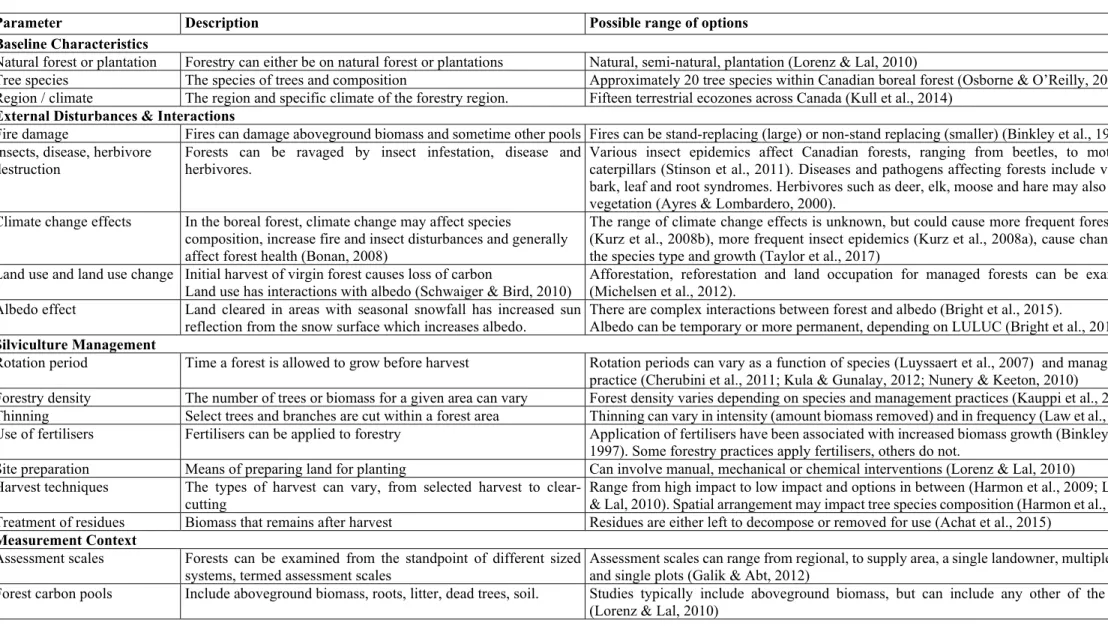
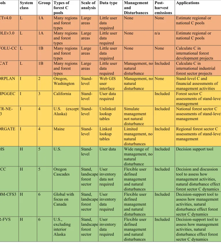
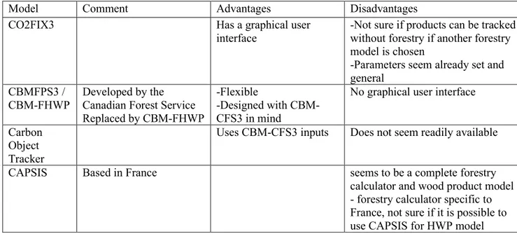
... 16 Table 2.2 – Product category rules (PCR) and normative standards covering wood and buildings (continued and end) ... 17 Table 2.3 – Overview of forestry parameters, with range of possibilities (parameters: Lorenz, and Lal (2010), categories: author) ... 22 Table 2.4 – Classification of forest carbon models and calculators, adapted from Zald et al. (2016), L = low (red), I = intermediary (yellow), H = high (green) ... 25 Table 2.5 – Comparison of wood product models (source: based on Brunet-Navarro et al. (2016))

... 28 Table 2.6 – Overview of recycling approaches ... 32 Table 4.1 – Ecosystem carbon costs at year 100 of simulation, in tC⋅m-3_{wood harvested ... 57}

Table 5.1 – Co-product outputs of sawmills for seven wood product types (% mass flows). CLT= cross-laminated timber, glulam= glue laminated timber, I-joist= engineered wood joist, LVL= laminated veneer lumber, OSB= oriented strand board, off-spec= off-specification, by-products= unspecified co-products... 68 Table 5.2 – End-of-life fate of clean wood (lumber) and composite/engineered wood (CLT, glulam, I-joist, LVL, OSB, plywood). “Construction” refers to waste occurring at the construction site at the beginning of a building’s life, whereas “demolition” is waste occurring at the end of a building life ... 69 Table 5.3 – Decay constant, k (year-1_{) for different regions and landfill types (ECCC, 2017) ... 73}

(16)

Table 5.5 – Initial post-demolition peak and cumulative CO2 and CH4 emissions for curves in

Figure 5.5, by province (NS = Nova Scotia, BC = British Columbia, ON = Ontario), scenario, and building lifespan. NS = Figure 5.5a, BC = Figure 5.5b and ON = Figure 5.5c ... 85 Table 6.1 – Relative time placement of unit processes into cradle-to-grave LCA of wood product, BL = building lifespan... 103 Table 6.2 – Parameters for base cases of four cradle-to-grave wood product cases (AB = Alberta, BC = British Columbia, SK = Saskatchewan, MB = Manitoba, ON = Ontario, QC = Quebec, NB = New Brunswick, NS = Nova Scotia, PE = Prince Edward Island, NL = Newfoundland, CLT = cross-laminated timber) ... 104

(17)

LIST OF FIGURES

Figure 2.1 – Lashof approach example. Storage of 1 tonne of CO2 for a period of 50 years for a

100-year time horizon. The blue line indicates an emission at time 0, while the red line indicates an emission following a storage period. The green shape represents the carbon benefit achieved from the storage period, beyond the 100-year time horizon (source: based on PAS2050 figures) ... 10 Figure 2.2 – Overview of the life cycle of wood used in a building, from a biogenic C perspective (thicker blue arrows indicate flow of biomass between stages, thinner blue arrows with “CO2”

or “CH4” indicate absorption or emission of those GHGs ... 19

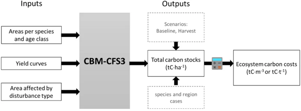
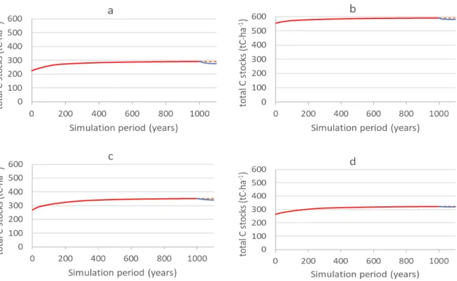
Figure 3.1 – General methodology flow diagram ... 36 Figure 4.1 – Schematic overview of inputs and outputs used with CBM-CFS3 ... 44 Figure 4.2 – Total carbon stocks of the baseline period from 0-1000 years (red line), followed by a harvest period from 1001-1100 years (blue). The dotted red lined represents the approximate steady-state value of the baseline period at 1000 years. a) Balsam fir (Abies balsamea), Quebec, Boreal Shield East, b) Lodgepole pine (Pinus contorta, British Columbia, Pacific Maritime, c) Western larch (Larix occidentalis), Alberta, Subhumid Prairies, d) White spruce (Picea glauca), New Brunswick, Atlantic Maritime. ... 50 Figure 4.3 – Ecosystem carbon cost, as net annual loss of carbon from the forest ecosystem to the atmosphere per cubic meter of wood harvested that year (tC⋅m-3_{wood) for four sample}

landscapes, as calculated with eq. 5a. The 0-100 period corresponds to the 1000-1100 period in Figure 4.2. a) Balsam fir (Abies balsamea), Quebec, Boreal Shield East; b) Lodgepole pine (Pinus contorta), British Columbia, Pacific Maritime; c) Western larch (Larix occidentalis), Alberta, Montane Cordillera; d) White spruce (Picea glauca), New Brunswick, Atlantic Maritime. Positive values represent a net C loss to the atmosphere, while negative values represent a net C gain from the atmosphere. ... 51 Figure 4.4 – Ecosystem carbon cost (ECC) by cubic metre of wood harvested for four common softwood tree species across Canada. The curves represent the interannual intervals of the harvest activity minus the carbon contained in the harvested wood, divided by the carbon

(18)

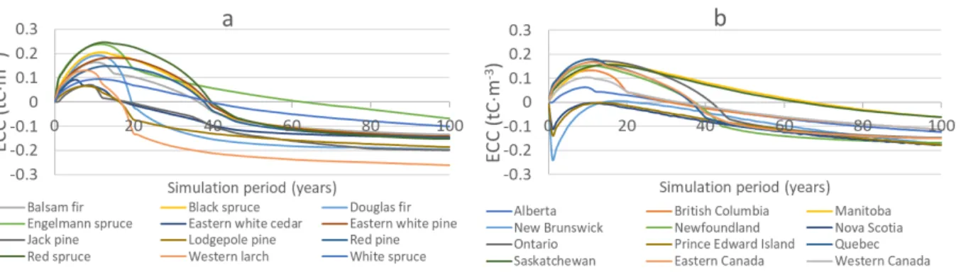
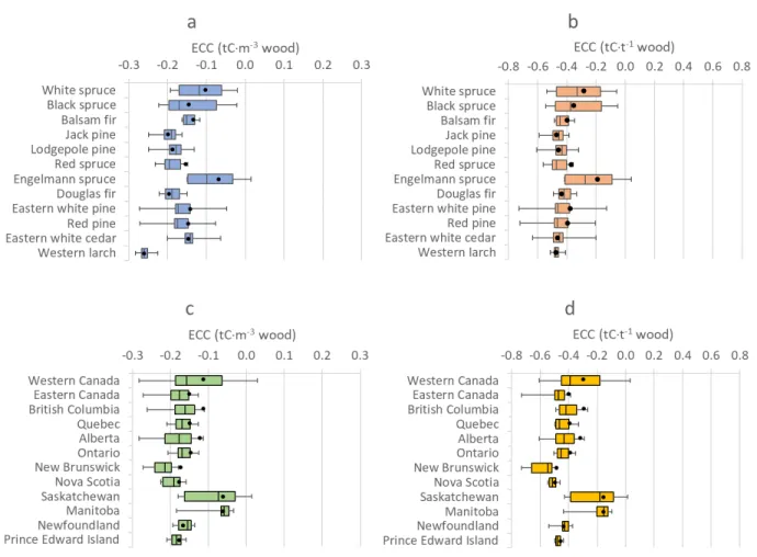
content of the annual harvest volume (see eq. 5a). a) Balsam fir (Abies balsamea), all occurrences, b) Lodgepole pine (Pinus contorta), all occurrences, c) Western larch (Larix occidentalis), all occurrences, d) White spruce (Picea glauca), all occurrences. The dark centre lines show the mean species and regions, the lighter bands ± 1 standard deviation, the dotted lines the minimum and maximum and the black dotted lines are the weighted average based on harvest volumes. ... 52 Figure 4.5 – Weighted mean of ecosystem carbon costs of harvest activity, by a) tree species b) provinces. Weights are harvested volumes. ... 54 Figure 4.6 – Ecosystem carbon costs at year 100 of simulation, for a) per tree species in tC⋅m-3

wood harvested, b) per tree species in tC⋅t-1_{wood harvested, c) per region in tC⋅m}-3_wood

harvested, d) per region in tC⋅t-1_{wood harvested. The carbon content of the dry wood ranges}

from 0.175 tC⋅m-3_{wood harvested (Eastern white cedar) to 0.300 tC⋅m}-3_{wood harvested}

(Western larch). The lower and upper error bars show the minimum and maximum values, while the lower bound of the box shows first quartile value, the middle line the median value and the upper bound the third quartile value. The round markers indicate the weighted mean values according to approximate annual wood harvest volumes. ... 56 Figure 4.7 – Modelled scenarios (baseline and harvest) for black spruce (Pinea mariana) and jack pine (Pinus banksiana) vs. flux tower data. BS = black spruce (Picea mariana), JP = jack spine (Pinus banksiana), wildfire (0-118 years) = landscape affected by annual fire starting from fire event in 1900 to present, harvest (1000-1100 years) = landscape affected by 100 years of annual fire and harvest following wildfire, 118 years after wildfire = point at present day 118 years after fire, 54 years after harvest = point at present day 54 years after harvest, weighted average model = weighted average of baseline and harvest scenarios, average flux tower = average of flux tower data from 2004-2010, flux tower 2004-2010 = annual averages from 2004-2010. Flux tower data from Fluxnet Canada / Canadian Carbon Program (Coursolle et al., 2012). ... 60 Figure 5.1 – System boundaries for wood product carbon flows. The processes contained within the dotted line are included in the model. The forest ecosystem and upstream forest harvest activities are developed in a previous study (Head et al., 2019a). Our implementation of the

(19)

model treats the “Leaves sawmill” and “Recycling and reuse” processes as being outside of the system scope. The figure only includes the biogenic carbon contained within the wood 67 Figure 5.2 – Change in carbon pools over time, for 1 m3_{lumber, Alberta, for four buildings}

lifespans (a) = 1 year, b) = 10 years, c) = 50 years, d) = 150 years). Deg, prod/cop= degradable portion of carbon in landfilled lumber main product/sawmill co-products, Non-deg, prod/cop= non-degradable portion of carbon in landfilled main product/sawmill co-products. Stored= carbon stored in building, Recycling, EOL= recycling of wood at end-of-life, Sold cop= co-products at sawmill sold to third parties ... 78 Figure 5.3 – Net carbon fluxes (kgC m-3_{product ⋅ year}-1_{) of CO}

2 and CH4 across: a) seven building

products (Alberta, building life = 50 years), b) provinces (lumber, building life = 50 years), c) building life (BL) years (Alberta, lumber) ... 79 Figure 5.4 – End fates of carbon for seven wood products at the sawmill (bioenergy and mill

landfill), at the construction site (site landfill) and end-of-life (EOL landfill). A) shows all end-of-life emissions, while b) shows just landfilling emissions. The EOL landfill proportion are calculated using landfilling rates for Alberta (91.5%). The wood (as carbon) sold from the sawmill is cut-off from the system and is not considered here, and differs by wood type (in kgC⋅m-3_{(% of total roundwood logs): lumber=219 (52%), plywood=105(36%), OSB=7 (3%),}

I-joists=151 (42%), CLT=178 (46%), LVL=181 (48%), glulam=214 (52%)) ... 81 Figure 5.5 – Net carbon fluxes (kg C/m3_{product) of CO}₂_{and CH}₄_{, comparing increased recycling}

policy (REC70% scenario) and increased landfill gas collection (LFG80% scenario) to the baseline scenario for lumber across a) high recycling rates (Nova Scotia), b) low landfill half-lives (British Columbia) and c) different building lifespans (Ontario). BL1 = building lifespan 1 year, BL50 = building lifespan 50 years, BL150 building lifespan 150 years ... 83 Figure 5.6 – Excerpt of Figure 5.5a (50-100 years) curves comparing kgC results with kgCO2 and

kgCH4, for each baseline, REC70% scenario and LFG80% scenario curves ... 84

Figure 6.1 – System boundaries of wood products along a life cycle timeline. The dotted large square denotes the system boundary. Thick black arrows show transport flows, while blue arrows do not include transport. Building Life appears in the timeline, but no elementary flows are considered. Yellow circles indicate elementary and intermediary flows. The green box

(20)

with “Natural gas production” is a unit process with an arrow directed towards “Wood processing” (and a negative sign) to indicate the substitution of hogfuel used as bioenergy at the wood processing unit process. ... 97 Figure 6.2 – Weighted average ecosystem carbon cost (ECC) from 0-100 years of historical forest management for 12 tree species ... 99 Figure 6.3 – Overall cradle-to-grave GHG emissions (kg CO2, kg CH4, kg N2O) profile for Eastern

SPF. Each point indicates a pulse emission in a given year. Outlier points are shown in the extensions to the graph in the positive and negative axis. ... 106 Figure 6.4 – Results for four case studies: E SPF, W SPF, DF-L, Cedar. Curves in a, b and c are shown for TH 0 to 500 years. a) GWIinst,(W⋅m-2⋅m-3 product), b) GWIcum (W⋅m-2⋅m-3

product), c) relative warming potential (kg CO2-eq⋅m-3 product), and d) relative warming

potential of E SPF, W SPF, DF-L, Cedar for three different TH, TH100, TH250, TH500 (kg CO2

-eq⋅m-3_{product). Case studies: E SPF = Eastern pine-fir, W SPF = Western}

spruce-pine-fir, DF-L = Douglas fir-Larch, ECC = ecosystem carbon cost. ... 107 Figure 6.5 – Ecosystem carbon costs (ECC) extended to 300 years of forest management for 4

species. E SPF = Eastern spruce pine fir, W SPF = Western spruce pine fir, DF-L = Douglas fir-Larch. Peak for Douglas fir curve extends to 1120 kg C⋅m-3_{wood harvested (not shown in}

graph) ... 109 Figure 6.6 – Comparing dynamic LCA results for four cases per m3_{wood product (Eastern SPF,}

Western SPF, Douglas fir-Larch, Cedar using top tree species) over a variable TH 0 to 500 years, using different ecosystem carbon cost (ECC) values determined after: 50, 75, 100 (default), 150 and 200 years of historical forest management. ... 110 Figure 6.7 – DLCA in kg CO2-eq⋅m-3 product of four wood cases, comparing default (blue line)

with incineration with grid mix substitution (red dotted line), incineration with marginal electricity substitution (green dotted line) and incineration with no energy substitution (yellow line). ... 111

(21)

Figure 6.8 – Net life cycle climate impacts of biogenic carbon (ECC, C wood uptake, EOL emissions) for lumber (kg CO2-eq⋅m-3 lumber). BL = building lifespan, 001, 010, 050, 100,

150 are building lifespan years. ... 113 Figure 6.9 – GWIinst results comparing black spruce (Quebec) from this study with Levasseur et al.

(22)

LIST OF SYMBOLS AND ABBREVIATIONS

AB Alberta

BC British Columbia BL Building lifespan

BSI British Standards Institute

CBM-CFS3 Carbon Budget Model of the Canadian Forest Service (software)

CBM-FHWP Carbon Budget Model Framework for Harvested Wood Products (software) CH4 Methane

CLT Cross-laminated timber CO2 Carbon dioxide

CRD Construction, renovation and demolition DCCI Dynamic climate change impacts

DF-L Douglas fir-Larch

DLCA Dynamic life cycle assessment ECC Ecosystem carbon cost

GHG Greenhouse gases

GTP Global temperature change potential GWIcum Cumulative global warming impact

GWIinst Instantaneous global warming impact

GWP Global warming potential

GWPbio Global warming potential of biomass-derived CO2

HWP Harvested wood products

IPCC Intergovernmental Panel on Climate Climate (of the United Nations) LCA Life cycle assessment

(23)

LCI Life cycle inventory

LCIA Life cycle impacts assessment LVL Laminated veneer lumber

MB Manitoba N2O Nitrous oxide NB New Brunswick NL Newfoundland NS Nova Scotia ON Ontario

OSB Oriented strand board PCR Product Category Rules PE Prince Edward Island

QC Quebec

SK Saskatchewan

SPF Spruce-pine-fir

TAWP Time-adjusted warming potential

TH Time horizon

(24)

LIST OF APPENDICES

Appendix A CORRIGENDUM OF ECOSYSTEM CARBON COST VALUES (ARTICLE 1) ... 162 Appendix B MODEL INPUT PARAMETERS (ARTICLE 1) ... 170 Appendix C MODEL INPUT PARAMETERS (ARTICLE 2) ... 176 Appendix D ADDITIONAL INFORMATION (ARTICLE 3) ... 180

(25)

Currently, buildings are estimated to contribute up to one-third of global carbon emissions, through their construction and operation (UNEP-SBCI, 2009). In order to minimise a building’s environmental impacts, it is essential to properly assess the impacts of different design choices. One common means of evaluating the environmental impacts of design choices is life cycle assessment (LCA). LCA is a method used to evaluate the potential environmental impacts of products, which in a building context could be used to evaluate the impacts of energy use, but could also be used to evaluate the impacts of using various types of building materials.

In Canada, wood is commonly used as a building material throughout the construction sector. However, the climate impacts of wood construction materials currently have limitations in how they are accounted for in life cycle assessment. Since biomass is considered to be part of the fast domain of the carbon cycle, the carbon fluxes between the atmosphere and biomass have been differentiated from the carbon fluxes originating from fossil sources. As such, the carbon from biomass, referred to as biogenic carbon, is said to have a net carbon balance of zero, meaning that the carbon sequestered by biomass is equal to the carbon eventually released by that biomass. This net zero carbon balance has been equated to a net zero climate change impact. Given the dynamic nature of carbon dioxide emissions and the resulting effect on the greenhouse gas effect and subsequently on climate change, the simplistic paradigm that carbon neutral equals climate neutral is being questioned.

There is an increasing body of scientific evidence that the actual climate impacts are dependent on many factors, such as storage time and emissions timing, the type of forest management practiced, and the end-of-life treatment of the wood product. However, to date there has been a lack of consensus on the issue surrounding the climate neutrality assumption. In addition, this issue has not yet been approached in a comprehensive and holistic manner that would consistently account for the climate impacts of wood over the entire life cycle of a building. As such, the aim of this research is to develop a method that reliably accounts for the uptake, emission and storage of biogenic carbon in the life cycle assessments of wood used in buildings in the Canadian context.

(26)

LITERATURE REVIEW

In order to contextualise the dissertation, the literature review will be presented in two main sections. The first section, on life cycle assessment and biogenic carbon, will introduce the reader to these concepts such as to give context to the biogenic carbon accounting issue. In the second section, wood products and methodological issues related to the calculation of their climate change impacts will be explored. This will address in detail the forestry, end-of-life disposal and timing aspects of the building life cycle, where biogenic carbon has important implications on climate change impacts.

2.1 Life Cycle Greenhouse Gas Assessment

At the very core of this research project, is life cycle assessment (LCA), a known and well-accepted tool that is used to assess the environmental impacts of a product throughout its product life cycle. In the context of this project, current LCA methodology concerning the accounting of biogenic carbon in climate change impact assessment, will be further broadened and developed. This section will introduce the reader to LCA, such as to provide context to the discussion on the accounting of biogenic carbon in wood products and buildings in later sections.

2.1.1

Introduction to Life Cycle Assessment

In its simplest terms, life cycle assessment (LCA) is a structured method that accounts for all resource inputs and emissions at every life cycle stage of a product or system, from its inception, resource extraction to its final disposal (European Commission, 2010c). It is a comprehensive approach that considers all quantifiable environmental impacts and in doing so strives to avoid the displacement of one environment impact for another (Bjørn et al., 2018d, p. 12). LCA can also be considered a decision-making tool, by comparing the environmental impacts of different production or process alternatives. The ISO 14044 standard on LCA defines four main phases (ISO, 2006a):

1. Goal and Scope Definition 2. Life Cycle Inventory (LCI)

3. Life Cycle Impact Assessment (LCIA) 4. Interpretation

(27)

2.1.1.1 Goal and Scope Definition

In the goal and scope definition, the LCA is framed and defined. More specifically, the context for the study and the intended audience are identified (Bjørn et al., 2018a, p. 68) and the product(s) or system(s) are described. The identification and description of the product(s) or system(s) includes determining the functional unit, system boundaries, how multifunctional processes will be treated, and the environmental impact categories (LCIA – see below) to be covered (Bjørn et al., 2018c, p. 76; European Commission, 2010c).

2.1.1.2 Life Cycle Inventory (LCI)

The objective of the life cycle inventory (LCI) phase is to collect and model data regarding all the processes in the studied product(s) or system(s) (European Commission, 2010c). In particular, in the LCI phase, all material, energy, emission flows flowing into and out of the product system (known as elementary flows) are considered. These are summed for all processes within the product life cycle and form the inventory for the studied product(s) or system(s) (Bjørn et al., 2018b, p. 118).

Some processes have more than one function and yield more than one product (coproducts), and thus they can be considered multifunctional (Bjørn et al., 2018c, p. 89). The process’ inventory must be attributed to the product considered by a given study’s function and functional unit. The ISO 14044 standard presents a hierarchy for solving multifunctional solutions (Bjørn et al., 2018c, p. 90; ISO, 2006b):

1. Attempt to subdivide multifunctional process inventory if separate inventories are available for each coproduct

2. Identify the most probable alternative production route for the other coproduct and expansion system boundaries to include this coproduct.

3. Allocate process inventory to primary product based on causal physical relationship, such as mass.

4. Allocate process inventory to primary product based on representative physical relationship such as energy density.

5. Allocate process inventory to primary product based on another parameter, such as economic relationship.

(28)

2.1.1.3 Life Cycle Impact Assessment (LCIA)

In the life cycle impact assessment (LCIA) phase, elementary flow inputs and outputs collected and modelled in the LCI phase are converted into potential environmental impacts and damages (European Commission, 2010c). The potential environmental impacts and damages that are calculated are those defined in the goal and scope definition. The conversion of environmental inputs and outputs to interpretable impact categories (referred to as LCIA), is accomplished using impact assessment methods. Since the early nineties, there have been several methods developed to quantify emissions into tangible potential environmental impacts (European Commission, 2010a). These methods combine extensive research and modelling of various environmental issues and damages. At their core, these methods can be distilled to usable conversion factors known as characterisation factors, which enable the conversion of resource inputs and emissions to mass equivalents of a reference substance (at the Midpoint level, e.g. kg CFC11-eq.1_{) or to recognised damage units (at the}

Endpoint level, e.g. DALY2_{). LCA methods are available to the LCA practitioner in the form of}

datasets and within LCA software programs.

2.1.1.4 Interpretation

Finally, in the interpretation phase, the results of the LCA are evaluated such that questions posed in the goal definition are answered (European Commission, 2010c). The relative environmental impact information can be used to make purchasing decisions, strategic decisions and can influence product design. Though the phases are typically carried out in the order given, LCA is actually an iterative process (European Commission, 2010c; ISO, 2006a). Based on preliminary results from the interpretation phase, for example, the goal and scope may be reviewed and adapted, which leads to changes in the subsequent LCI and LCIA phases.

1_{Kilogram equivalents of trichlorofluoromethane (CFC11), a reference substance for impact category, Ozone depletion}

potential

(29)

2.1.2 The Carbon Cycle

Carbon is contained within all living organisms, in soil and in fossilised organisms. Cumulatively, carbon-based emissions are part of the global carbon cycle. The carbon cycle consists of carbon reservoirs, as well as the exchanges of carbon fluxes between them (Ciais et al., 2013).

Two main domains have been identified within the carbon cycle, based upon the turnover rates within the reservoirs. The first domain is considered the fast domain, in which a large amount of rapid exchanges take place. These exchanges occur between the atmosphere, oceans, vegetation, soils and freshwater. The second domain is considered the slow domain, in which carbon exchanges occur slowly (in periods of over 10,000 years) between geological formations and the atmosphere. In nature, without human intervention, the fluxes occurring within the slow domain are small. Since the advent of the industrialised era, carbon has been extracted from the geological reservoirs in the form of fossil fuels. The extraction and combustion of these fossil fuels has led to a large transfer of carbon from the slow domain of the carbon cycle to the fast domain, and thus the perturbation of the global carbon cycle (Ciais et al., 2013).

2.1.3 The Greenhouse Gas Effect and Climate Change Metrics

Through mechanisms such as combustion, decomposition and weathering, carbon-containing substances emit greenhouse gases such as carbon dioxide and methane. Greenhouse gases (GHG) are substances which tend to trap heat in the atmosphere, increasing the greenhouse gas effect. The greenhouse gas effect is a mechanism caused by the combination of solar radiation and greenhouse gases. One third of this energy is reflected back towards space, while the two-thirds is absorbed by the surface of the earth and the atmosphere (Cubasch et al., 2013). The absorption of this solar energy is crucial to the life on earth, which would otherwise be entirely frozen.

The accumulation of additional heat has been directly correlated to an increase in global temperatures and to overall change in the earth’s climate. Several authors have proposed different metrics for quantifying climate change impacts. The most commonly used metric used by the Intergovernmental Panel on Climate Change (IPCC) is the global warming potential (GWP). The GWP is defined as the time integrated radiative forcing as a result of a pulse emission of a greenhouse gas relative to a pulse emission of carbon dioxide (Myhre et al., 2013):

(30)

𝐺𝐺𝐺𝐺𝐺𝐺𝑖𝑖(𝐻𝐻) = ∫ 𝑅𝑅𝑅𝑅𝑖𝑖(𝑡𝑡)𝑑𝑑𝑡𝑡 𝐻𝐻 0 ∫ 𝑅𝑅𝑅𝑅𝐶𝐶𝐶𝐶2(𝑡𝑡)𝑑𝑑𝑡𝑡 𝐻𝐻 0 =_{𝐴𝐴𝐺𝐺𝐺𝐺𝐺𝐺}𝐴𝐴𝐺𝐺𝐺𝐺𝐺𝐺𝑖𝑖(𝐻𝐻) 𝐶𝐶𝐶𝐶2(𝐻𝐻) (1)

Where H is the time horizon, t is time, RF is radiative forcing, i is a given greenhouse gas, and AGWP is absolute global warming potential.

The GWP indicator is a midpoint indicator. All substances having a global warming potential have been normalised with the impact score of the reference substance, carbon dioxide (Forster et al., 2007).

Another metric that has been proposed is the Global Temperature change Potential (GTP) (Shine et al., 2005). GTP measures the impact of climate change further down in the cause and effect chain. It is defined as the “change in global mean surface temperature at a chosen point in time in response to an emission pulse relative to that of CO2 (Myhre et al., 2013). Mathematically, GTP can be

expressed as: 𝐺𝐺𝐺𝐺𝐺𝐺𝑖𝑖(𝑡𝑡) =_{𝐴𝐴𝐺𝐺𝐺𝐺𝐺𝐺}𝐴𝐴𝐺𝐺𝐺𝐺𝐺𝐺𝑖𝑖(𝑡𝑡) 𝐶𝐶𝐶𝐶2(𝑡𝑡) = ∆𝐺𝐺𝑖𝑖(𝑡𝑡) ∆𝐺𝐺𝐶𝐶𝐶𝐶2(𝑡𝑡) (2) Where t is time, i is a given greenhouse gas, AGTP is absolute global temperature potential and ∆T is the

change in temperature.

While GTP and GWP both express results in terms of kg CO2-equivalents, there are differences

between these metric types. GTP yields results that more closely model actual impacts than the radiative forcing approach. In addition, GTP is usually appropriate for use in assessing the impacts at the end of a targeted period of time than other metrics. However, since GTP is based on the response time of the climate to greenhouse gas emissions, the metric can result in more uncertainty than a metric like GWP that is further upstream in the cause and effect chain (Levasseur et al., 2016a; Levasseur et al., 2016b; Myhre et al., 2013).

These metrics can be expressed at different time horizons, allowing for short- and long-term climate change impacts to be quantified. Typically, and historically, the GWP 100-year time horizon has been the default indicator used in quantifying the climate change impacts of greenhouse gas emissions. However, the latest recommendations are to use two indicators in order to cover short-term and long-short-term climate change. For the short-short-term climate change effects that target warming rates, GWP100 is recommended as it considers GHGs that decay rapidly. For the long-term climate

(31)

change effects that target long-term temperature rise, GTP100 is recommended as it considers similar impacts to those of GWP250 or GWP500, for example (Levasseur et al., 2016b).

2.1.4 Biogenic Carbon and Neutrality

The concepts of fast and slow domains within the carbon cycle were introduced in section 2.1.2. Plant matter and organisms currently or recently living, also known as biomass, are considered to be part of the fast domain of the carbon cycle. As a result of the speed at which biomass typically cycles between reservoirs, a distinction has been made for carbon emissions from so-called biogenic sources. The reason for this has to do with the fact that biogenic carbon emissions originate from biomass that has previously but recently sequestered carbon dioxide from the air.

Since the amount sequestered and the amount released are more or less identical, several papers and guidelines on LCA and carbon footprinting have assumed that the net carbon balance and thus the climate change impacts are zero (Johnson, 2009; Rabl et al., 2007; Searchinger et al., 2009). However, several publications have recently shown that this assumption could lead to accounting errors (Garcia & Freire, 2014; Røyne et al., 2016; Searchinger et al., 2009; Vogtländer et al., 2013). Depending on the origin of wood and how it is harvested, forest products can result in emissions, net zero emissions or sequestration (Berndes et al., 2016). Røyne et al. (2016) found that including biogenic carbon accounting could increase the climate change impacts by up to 44% by considering the climate impacts of both biogenic and fossil carbon in end-of-life processes of wood products. In particular, accounting errors occur as a result of the application of the carbon neutrality assumption. First, if the neutrality assumption were applied to managed forests, it would mean that there would be no difference to the carbon footprint whether a tree was left standing or harvested (Johnson, 2009). Second, carbon neutrality can also stem from a consideration of carbon from the forest assessment scale or a given harvest pattern, in which harvest is balanced by regrowth of new trees (Lemprière et al., 2013; McKechnie et al., 2011). Third, the carbon neutrality assumption does not consider the time needed to offset carbon emissions, as it may take years to counteract the carbon that has accumulated in the atmosphere since the release of a greenhouse gas (Cherubini et al., 2011; Helin et al., 2013; Lemprière et al., 2013; McKechnie et al., 2011; Zanchi et al., 2010).

Several authors have developed approaches for improving the accounting of biogenic carbon of bioenergy (Cherubini et al., 2011; Kendall et al., 2009; Repo et al., 2011; Zanchi et al., 2010). Other

(32)

authors have used a carbon neutrality factor in order to quantify the relative greenhouse gas emissions savings of bioenergy (Schlamadinger et al., 1995; Zanchi et al., 2010). McKechnie et al. (2011) integrated forest carbon analysis and life cycle assessment in order to evaluate greenhouse gas emissions of the use of forest biomass for bioenergy over time. The development of approaches in life cycle assessment for characterising biogenic carbon have been largely in the area of forest biomass used in bioenergy. However, a few studies have included methods for biogenic carbon accounting for wood products (Cherubini et al., 2012; Pingoud et al., 2011).

2.1.5 Emissions Timing

Typically in LCA, emissions are summed over the whole life cycle and characterised in LCIA without considering when in time the emissions took place. However, over twenty years ago researchers began acknowledging that the timing of emissions can have an effect on environmental impacts (Owens, 1997; Reap et al., 2008). Since the turn of the century, several methods have been proposed to address emissions timing (BSI, 2011b, 2011c; European Commission, 2010b; Fearnside, 2002; Guest et al., 2013b; Kendall, 2012; Levasseur et al., 2010; Moura Costa & Wilson, 2000; Vogtländer et al., 2013). However, the climate benefits of regarding emissions timing have been controversial (Brandão & Levasseur, 2011; Brandão et al., 2013). As such, LCA studies do not typically include the impacts of carbon storage or the timing of carbon emissions and uptakes, as shown by Røyne et al. (2016) who found that the majority of LCA studies do not include the timing of emissions. Emissions timing is especially relevant in the case of biomass life cycles, particularly when biomass is used in applications within the anthroposphere with relatively long lifetimes, such as buildings. The biogenic carbon uptake in the biomass and its eventual release as greenhouse gas emissions can take place over relatively long timescales, which can have an impact on the climate change potentials.

In conventional LCAs, emissions and impacts time horizons do not necessarily have to cover the same sequence of years. However, the climate change outcomes may differ depending on when the accounting period begins (Levasseur et al., 2013), the choice of which should be guided by the objective and context of a study (Berndes et al., 2016). As such, at the outset of a life cycle assessment, time horizons for both the product life cycle emissions as well as the impact assessment are chosen. Although the time horizon is often chosen relative to the lifespan of the product

(33)

considered, this is not always the case. In fact, the choice of a time horizon is considered to be subjective (Fearnside, 2002). With GWP impacts, typically 20, 100 or 500 year time horizons are chosen (Forster et al., 2007), each corresponding to a different value perspective. Jørgensen, and Hauschild (2012) found that both short and long time horizons are necessary for addressing both the acute and long-term climate impacts of temporary carbon storage. However, as shown by Levasseur (2015), the choice of time horizon has an important effect on climate change results.

2.1.5.1 Temporal Approaches at the Life Cycle Impact Assessment Level

Several methods have been proposed over the course of the last fifteen years to address the issue of emissions timing. Brandão et al. (2013) presented a review of the most viable approaches, as a result of an expert workshop that was convened on the topic of carbon sequestration and temporary storage. A brief introduction to the most relevant methods is given below, and summarised in Table 2.1. Two similar approaches using what is known as the tonne-year baseline, were developed around the same time (in the year 2000). The tonne.year baseline approach uses the radiative forcing (climate impact) of 1 tonne of carbon dioxide released at time zero, over a 100-year time horizon. The integral of this baseline curve is calculated in terms of tonne.years.

Fearnside et al. (2000) proposed a method known as the Lashof method, which attempted to evaluate the effects of delaying emissions following temporary storage. The method makes use of the curve of cumulative atmospheric mass loading of carbon as a result of a pulse emission, as a function of time. The integral of the curve gives the cumulative atmospheric mass loading in tonne.years. When an emission is delayed, this curve is offset by the corresponding number of years that the emission is delayed (see Figure 2.1). The part of the curve extending past the fixed time horizon is no longer considered and corresponds to the benefits related to the storage of that quantity of carbon.

The other method based on the tonne.year approach is known as the Moura-Costa method (Moura Costa & Wilson, 2000). The Moura-Costa method translates the tonne-years into years of carbon storage, and further allocates this stored carbon credit per year. Thus, despite having similar baselines, the Lashof and Moura-Costa approaches differ substantially in terms of the amount of emission benefit attained. They are also both very dependent upon the time horizon chosen.

(34)

Figure 2.1 – Lashof approach example. Storage of 1 tonne of CO2 for a period of 50 years for a

100-year time horizon. The blue line indicates an emission at time 0, while the red line indicates an emission following a storage period. The green shape represents the carbon benefit achieved from

the storage period, beyond the 100-year time horizon (source: based on PAS2050 figures) The approach uses weighting factors, which are related to the timing of the emissions (BSI, 2008). If the emissions occurred within 2-25 years of the product manufacture, the weighting factor was calculated using a linear approximation of the Lashof method, characterised by:

𝐺𝐺𝑊𝑊𝑊𝑊𝑊𝑊ℎ𝑡𝑡𝑊𝑊𝑡𝑡𝑊𝑊 𝑓𝑓𝑓𝑓𝑓𝑓𝑡𝑡𝑓𝑓𝑓𝑓 = 0.76 × 𝑡𝑡₁₀₀ 0 (3) t0 = number of years the full carbon storage benefit of a product exists after the products is created.

Whereas, the weighting factor for emissions occurring beyond 25 years is calculated as:

𝐺𝐺𝑊𝑊𝑊𝑊𝑊𝑊ℎ𝑡𝑡𝑊𝑊𝑡𝑡𝑊𝑊 𝑓𝑓𝑓𝑓𝑓𝑓𝑡𝑡𝑓𝑓𝑓𝑓 =∑₁₀₀100𝑖𝑖=1𝑥𝑥𝑖𝑖 (4)

i = each year of carbon storage, x = proportion of total storage remaining in any year i

The British Standards Institute (BSI) published an update to the standard in 2011 (BSI, 2011a), which now states that the emissions timing is optional.

The European Union’s Joint Research Council published a series of guidelines for life cycle assessment in 2010, known collectively as the ILCD handbook (European Commission, 2010a). The ILCD handbook method follows the same emissions delay approach used in the Lashof method,

(35)

where emissions occurring after the defined time horizon are subtracted from the amount of carbon originally emitted. Unlike the Lashof method, the ILCD handbook method uses a linear approximation, which is carried by multiplying avoided emissions by the GHG 100-year characterisation factor, the number of years delayed (years that carbon is stored) and the factor -0.01 kg CO2-eq/year.kg CO2-eq. Any emissions occurring after 100 years are not included in the LCA

results but are documented separately.

One of the more recent approaches developed to account for emissions timing has been the Dynamic LCA method (Levasseur et al., 2010). This method, which is based on the IPCC’s absolute global warming potential (AGWP) equation integrated continuously through a fixed time horizon, allows for the calculation of a radiative forcing impact at any point in time. Dynamic characterisation factors (DCF) are used in combination with a temporally differentiated emissions inventory to calculate the instantaneous global warming impact, GWIinst,

𝐺𝐺𝐺𝐺𝐺𝐺𝑖𝑖𝑖𝑖𝑖𝑖𝑖𝑖(𝑡𝑡) = ∑ �𝑘𝑘𝑊𝑊𝐶𝐶𝐶𝐶𝑖𝑖𝑖𝑖=𝑘𝑘 2(𝑘𝑘) ∙ 𝐷𝐷𝐶𝐶𝑅𝑅𝐶𝐶𝐶𝐶2(𝑡𝑡 − 𝑘𝑘)� + ∑ �𝑘𝑘𝑊𝑊𝐶𝐶𝐻𝐻𝑖𝑖𝑖𝑖=𝑘𝑘 4(𝑘𝑘) ∙ 𝐷𝐷𝐶𝐶𝑅𝑅𝐶𝐶𝐻𝐻4(𝑡𝑡 − 𝑘𝑘)� +

∑ �𝑘𝑘𝑊𝑊𝑁𝑁𝑖𝑖𝑖𝑖=𝑘𝑘 2𝐶𝐶(𝑘𝑘) ∙ 𝐷𝐷𝐶𝐶𝑅𝑅𝑁𝑁2𝐶𝐶(𝑡𝑡 − 𝑘𝑘)� (5)

Each summed expression represents the radiative forcing of all pulse emissions of a given GHG in a given year. The pulse emissions (in kg GHG) in year k are multiplied by GHG-specific characterisation factors for every time step (t – k).

The cumulative radiative forcing (GWIcum) of all GHG pulse emissions is calculated for all years

from 0 – t and is represented by,

𝐺𝐺𝐺𝐺𝐺𝐺𝑐𝑐𝑐𝑐𝑐𝑐(𝑡𝑡) = ∑𝑖𝑖𝑘𝑘=0𝐺𝐺𝐺𝐺𝐺𝐺𝑖𝑖𝑖𝑖𝑖𝑖𝑖𝑖(𝑡𝑡) (6)

Cumulative forcing results are translated into DLCIA (dynamic life cycle impact assessment) scores in terms of kgCO2-eq., by dividing the GWIcum by the cumulative radiative of 1 kg of CO2 emitted

at time zero to the given time horizon TH, 𝐷𝐷𝐷𝐷𝐶𝐶𝐴𝐴 = 𝐺𝐺𝐺𝐺𝐺𝐺𝑐𝑐𝑐𝑐𝑐𝑐(𝑇𝑇𝐻𝐻)

∫₀𝑇𝑇𝑇𝑇𝑅𝑅𝑅𝑅_{𝐶𝐶𝐶𝐶2}∙𝐶𝐶(𝑖𝑖)_{𝐶𝐶𝐶𝐶2}𝑑𝑑𝑖𝑖 (7)

The denominator of the DLCA equation represents the cumulative radiative forcing of a single 1 kg CO2 pulse emission. TH represents the time horizon chosen for the study. In essence, the equation

(36)

over the course of the life cycle of the product in question. An Excel-based tool called DYNCO2

(Levasseur, 2013) was developed to provide a calculation platform for Dynamic LCA.

Kendall (2012) developed an approach known as the Time-Adjusted Warming Potential (TAWP), which is based on the IPCC GWP model. This method is identical to the Dynamic LCA method, though instead of allowing flexibility in time horizons, the method fixes five specific time horizons (20, 30, 50, 100, 500 years).

GWPbio is a concept that combines the Bern carbon cycle model and a Gaussian growth curve in

order to quantify the climate impact of biomass energy emissions, which was originally developed by Cherubini et al. (2011) to calculate characterisation factors for bioenergy. The approach is dependent on the number of years required to regrow the biomass and uses three fixed time horizons: 20, 100 and 500 years. Guest et al. (2013b) further adapted this method to include a product lifetime for the use phase of the biomass being used as bioenergy. The model oversimplifies a few aspects about the forestry phase, including species, growing region and type of forest management. In addition, the model is based on the end-of-life combustion of the biomass, which excludes any other end-of-life waste management outcomes, such as recycling or landfilling.

One of the most recent methods of approaching emissions timing and temporal incongruity in LCAs was proposed by Yuan et al. (2015). The method was developed in order to include several perspectives not necessarily taken into consideration in existing methods and consists of a procedure, involving: 1) calculating the temporal scale of LCA, 2) compiling the temporally differentiated life cycle emissions, 3) modelling the actual environmental fate of emissions, 4) discounting emissions to selected reference time point, 5) aggregating discounted emissions at the reference time point. In addition to these general timing approaches, other authors have proposed methods for accounting for the delay of a specific greenhouse gases, such as Sevenster (2014) who developed a linear approximation of the dynamic LCA method for methane. Despite the practicality of such an approach for specific activities, such as the release of methane emissions from landfill, approaches with broader range of applications are more useful for modelling a variety of life cycle scenarios.

Of the approaches presented, the Lashof and Moura-Costa approaches are simple, focused on temporary storage but are not necessarily appropriate for consistent application to life cycle assessment. The ILCD and PAS2050 approaches are also quite user-friendly and straightforward,

(37)

however due to their reliance on a 100-year time horizon, the fact that they ignore sequestration dynamics and that they do not provide GHG-specific emission delay credits, they make poor choices for in-depth application to the life cycle of wood products. Despite purporting to address temporal issues in LCA, Yuan et al. (2015) approaches time using a discounting methodology but does not actually provide specific means for addressing time horizons or emission delays. Finally, the DLCA and TAWP approaches both consider sequestration dynamics, are GHG-specific, and offer the choice of time horizon (DLCA: any, TAWP: choice of 5), which makes these methods applicable to a large range of cases and complexity levels.

The climate change outcomes may differ depending on when the accounting period begins (Levasseur et al., 2013), the choice of which should be guided by the objective and context of a study (Berndes et al., 2016). In testing four different approaches that consider emissions timing and temporary carbon storage, Røyne et al. (2016) found that the approaches had climate benefits ranging from 8% (for the GWPbio approach - Guest et al. (2013b)) to 70% (for a discounting approach using

a 1% discount rate) of the life cycle impacts of a wood construction. The ILCD approach (European Commission, 2010b) and the dynamic life cycle approach (Levasseur et al., 2010) have climate benefits somewhere in between these two extremes (31-38%). The emissions timing methods described above are summarised in Table 2.1, in terms of their calculation approach, time horizon and advantages and disadvantages.

(38)

Table 2.1 – Summary of emissions timing methods. CAML = cumulative atmospheric mass loading, TH = time horizon

Method Calculation approach Time

Horizon Advantages Disadvantages Main reference Lashof -Uses curve of CAML of carbon as a result

of a pulse emission, as a function of time -Integral of CAML = tonne.years -Emissions delay = offset curve -Uses temporal cut-off

Any Simple Choice of TH crucial has large impact on results and conclusions

Fearnside et al. (2000)

Moura-Costa -Uses equivalence factor yearly crediting (tonne.year) -Based on CAML value of single CO2

emission

-Uses temporal cut-off

Any Simple May not be suitable for

LCAs Moura Costa, and Wilson (2000) ILCD -Linear approximation of Lashof method,

subtracting the emission that takes place beyond the time period

100

years Simple Linear -Does not consider sequestration dynamics -Credits for delayed emissions same for all GHG emissions.

European Commission (2010c) PAS2050 -Linear approach based on Lashof method

for two different times: 2-25 years and 25+ years after product manufacture

100

years Simple Linear -Does not consider sequestration dynamics -Credits for delayed emissions same for all GHG emissions. BSI (2008, 2011c) Dynamic LCA (DLCA)

Calculation of global warming impacts at every point of time where emissions occur, for every GHG, over the course of the life cycle of the product in question.

Any -Considers sequestration dynamics

-GHG-specific approach -TH consistent

(emissions & impacts) -Choice of any TH

Choice of TH and temporally differentiated emissions can make choice for decision-maker more difficult (Dyckhoff & Kasah, 2014; Levasseur et al., 2013)

Levasseur et al. (2010)

TAWP Calculation of global warming impacts at every point of time where emissions occur, for every GHG, over the course of the life cycle of the product in question.

-Characterisation factors calculated for each emission year 20, 30, 50, 100, 500 years -Considers sequestration dynamics -GHG-specific approach -Limits choice of TH -Only considers 5 TH –

could limit outcomes Kendall (2012)

Yuan et al.

(2015) Proposed a five-step method, which is distinguished by the use of discounting N/A Addresses temporal differentiation of emissions

-No specific method for dealing with TH and emission delays

-Requires high level detail on timing of emissions

Yuan et al. (2015)

2.1.5.2 Temporal Differentiation of the Life Cycle Inventory

In order to practically apply most of the temporal approaches to the life cycles of products, the specific timing of each individual emission must be determined. Several authors have explored the temporal differentiation of life cycle inventories (LCI) in order to be able to apply temporal methods (Beloin-Saint-Pierre et al., 2014; Collet et al., 2013; Collinge et al., 2013; Pinsonnault et al., 2014;

(39)

Yuan et al., 2015). Collet et al. (2013) developed a method for determining whether considering dynamic life cycle inventories has an overall impact on LCIA results, and whether they are worth applying. Beloin-Saint-Pierre et al. (2014) proposed the enhanced structural path analysis (ESPA) method in order to apply temporal differentiation on a mass scale (database-level) to elementary and process flows. Within the context of global warming impacts, Pinsonnault et al. (2014) sought to determine the sensitivity of adding temporal information to LCIA results by using the ESPA method (Beloin-Saint-Pierre et al., 2014). They generated temporally differentiated LCIs for every product in the ecoinvent 2.2 database and found that temporal information can be particularly relevant for products containing biomass. In their temporal LCIA method, Yuan et al. (2015) also described steps in order to temporally differentiate at the LCI level. More recently, Tiruta-Barna et al. (2016) and Cardellini et al. (2018) developed methods that generate temporally differentiated LCIs using software programs.

2.2 Carbon Accounting for Wood used in Building and Construction

2.2.1 Whole Wood Life Cycle Considerations

LCA practitioners and industry instead tend to rely on existing perspectives and approaches that have reached a certain consensus within the LCA community, such as product category rules (PCR) and normative standards. Table 2.2 gives an overview of the PCRs and normative standards covering wood and buildings as well as their treatment of both biogenic carbon and emissions timing.

(40)

Table 2.2 – Product category rules (PCR) and normative standards covering wood and buildings Region PCR/ Standard Biogenic CO2 Allocation Timing LUC North

America North American Structural and Architectural Wood Products (FPInnovations, 2015); Inputs as -1 and outputs as 1, characterised as fossil C = net zero, carbon storage can be provided separately

Multi-output processes: ∆$ coproducts:

low: mass, volume high (>10%): economic Allocate by physical flows for biogenic carbon, water, energy

Presented as separate GWP indicator with reference methodology LUC reported separately North American Pressure-treated Wood Products (ASTM/ICC-ES, 2016);

Physical relationship between co-products: by mass

No relationship: equal division among co-products

Not stated Not mentioned

United

Kingdom PCR for Construction Products EPD (BRE, 2014).

Inputs as -1 and outputs as 1, characterised as fossil C = net zero, no carbon storage

Has its own allocation preference hierarchy (decision tree)

Not stated Included as per IPCC

guidelines for national GHG inventories PAS 2050 (BSI, 2011c); Inputs as -1 and

outputs as 1, carbon storage can be provided separately

Avoid allocation, otherwise allocate by physical property (mass, etc.), as a last resort by economic or other relationship.

Reported separately using method provided GHGs allocated to goods/services for 20 years after the land use change Norway Wood and wood-based

products for use in construction (The Norwegian EPD Foundation, 2013b); Inputs as -1 and outputs as 1, carbon storage can be provided separately

Allocation by volume or mass if subdivided or little value difference. If not subdivided and large value differences, economic allocation shall be used. Can be calculated by recognised method, but reported separately None mentioned

Building boards (The Norwegian EPD Foundation, 2013a);

Allocation according to mass or volume. At large value

differences (>20%), economic allocation shall be used.

LUC reported separately

France AFNOR BP X30-323 (ADEME & AFNOR, 2011).

Inputs as -1 and outputs as 1, carbon storage can be provided separately

Avoid allocation, otherwise allocate by physical property (mass, etc.), as a last resort by economic or other relationship.

Time-weighted average for storage and delay 0-100 years. Included as per IPCC guidelines for national GHG inventories Germany Product Category Rules

for Building-Related Products and Services (Institut Bauen und Umwelt, 2014)

Not stated ∆$ coproducts: low: mass, volume

otherwise economic allocation Allocate by physical flows for biogenic carbon, water, energy

Not stated None mentioned