On Line Trace Synchronization for Large Scale Distributed Systems

ON LINE TRACE SYNCHRONIZATION FOR LARGE SCALE DISTRIBUTED SYSTEMS

MASOUME JABBARIFAR

D´EPARTEMENT DE G´ENIE INFORMATIQUE ET G´ENIE LOGICIEL ´

ECOLE POLYTECHNIQUE DE MONTR´EAL

TH`ESE PR´ESENT´EE EN VUE DE L’OBTENTION DU DIPL ˆOME DE PHILOSOPHIÆ DOCTOR

(G ´ENIE INFORMATIQUE) NOVEMBRE 2013

c

´

ECOLE POLYTECHNIQUE DE MONTR´EAL

Cette th`ese intitul´ee :

ON LINE TRACE SYNCHRONIZATION FOR LARGE SCALE DISTRIBUTED SYSTEMS

pr´esent´ee par : JABBARIFAR Masoume

en vue de l’obtention du diplˆome de : Philosophiæ Doctor a ´et´e dˆument accept´ee par le jury d’examen constitu´e de :

Mme BOUCHENEB Hanifa, Doctorat, pr´esidente

M. DAGENAIS Michel, Ph.D., membre et directeur de recherche M. GAGNON Michel, Ph.D., membre

I dedicate my dissertation work to :

my loving parents, Batoul and Norouzali whose words of encouragement while I am far away of them and they miss me a lot,

my husband, Alireza, has never left my side and supported me throughout the process with his special love,

my beautiful princess daughter, Liana, whose smile is my everything

ACKNOWLEDGEMENTS

I would like to express my deep and sincere gratitude to my supervisor Professor Dr. Michel Dagenais for his endless support, understanding, kindness, and great supervision. His guidance and ideas opened new doors into new aspects of distributed systems tracing for me. He also gently added some constraints and restrictions into the method of thinking which have been very beneficial and accelerated my research process. During my PhD studies in Ecole Polythechnique de Montreal, I learned a lot from him not only about research but also about life.

Many thanks go to the committee members who were more than generous with their expertise and precious time. A special thanks to Dr. Hanifa Boucheneb, committee chairman, for her countless hours of reflecting, reading, encouraging, and most of all patience throughout the entire process. Thank you Dr. Michel Gagnon, Dr. Dhrubajyoti Goswami, and Dr. Robert Legros for agreeing to serve on my committee.

Thanks to Ericsson and the Natural Sciences and Engineering Research Council of Canada for funding this research.

I would like to thank my friends and colleagues at the DORSAL laboratory of the depart-ment of Computer and Software Engineering. All of you have been my best cheerleaders.

I wish to thank my mother Batoul Tabaghlou-Sorkhab and my father Norouzali Jabba-rifar. No words can express and no act of gratitude can relay what their love and support have meant to me. I hope they accept this as an indication of my heartfelt appreciation for everything they are.

I would like to thank my brothers Rasoul and Davoud, my sisters Farkhonde, Soraya, and Fahime and their lovely families, my nephews Vahid and Saeed and their nice spouses, Ali, and Mohammad, and finally my nieces Maryam, Pegah, Maedeh, Mahya, Zahra, Parastou, and Dina. Without their support and encouragement, my efforts to complete this dissertation would not have been possible.

I am very thankful to my mother-in-law and father-in-law, Parvin and Khanali Shameli-Sendi. I am also grateful to my brothers-in-law Mohammad and his family, and Sajad, and my sisters-in-law Zahra and Fatemeh for their unconditionally loving and supportive energy at all times.

Finally, but most importantly, I am indefinitely indebted to my husband, Alireza, who has put up with me for reasons not always obvious, endured countless sacrifices so that I can follow my dreams and supported me in any way that he could. I owe all of my accomplishments to him.

R´ESUM´E

Les syst`emes distribu´es en r´eseau fournissent une plate-forme informatique polyvalente pour soutenir diverses applications, telles que des algorithmes de routage dans les r´eseaux de t´el´ecommunication, les syst`emes bancaires dans les applications de r´eseau, les syst`emes de contrˆole d’a´eronefs dans le contrˆole de processus en temps r´eel, ou le calcul scientifique, y compris les grilles et grappes de calcul en calcul parall`ele. Ces syst`emes sont g´en´eralement supervis´es afin de d´etecter, de d´eboguer et d’´eviter les probl`emes de s´ecurit´e ou de perfor-mance. Un outil de tra¸cage est une des m´ethodes les plus efficaces et pr´ecises, avec laquelle toutes les informations d´etaill´ees pour chaque noeud individuel dans le syst`eme peuvent ˆetre extraites et ´etudi´ees.

Typiquement, une tˆache ´enorme est divis´ee en de nombreuses tˆaches, qui sont distribu´ees et ex´ecut´ees sur plusieurs ordinateurs coop´erant en r´eseau. Ainsi, afin de contrˆoler la fonc-tionnalit´e des syst`emes distribu´es actuels, toutes les informations sont collect´ees `a partir de plusieurs syst`emes et appareils embarqu´es pour une analyse et une visualisation `a la fois en ligne et hors ligne. Cette information de tra¸cage, g´en´er´ee `a un rythme effarant, est livr´ee avec estampilles de temps g´en´er´ees localement sur chaque noeud. Ces estampilles sont g´en´ erale-ment fond´ees sur des compteurs de cycle, avec une granularit´e du niveau de la nanoseconde. Toutefois, les horloges de chaque noeud sont ind´ependantes et donc asynchrones les unes des autres. N´eanmoins, les utilisateurs s’attendent `a voir la sortie de l’analyse en temps r´eel, sur un axe de r´ef´erence de temps commun, afin d’ˆetre en mesure de diagnostiquer les probl`emes plus facilement.

La port´ee de l’oeuvre propos´ee ici est la synchronisation efficace et en direct de traces g´en´er´ees dans un environnement de grande grappe d’ordinateurs avec des estampilles de temps de granularit´e du niveau de la nanoseconde, produites par des horloges non synchronis´ees. Par ailleurs, le mod`ele de trafic du r´eseau, le nombre de noeuds informatiques disponibles et mˆeme la topologie du r´eseau peuvent changer. En effet, les grands centres de donn´ees roulent un ensemble diversifi´e et en constante ´evolution d’applications. Les noeuds peuvent ´echouer ou revenir en ligne `a tout moment, et mˆeme le r´eseau peut ˆetre reconfigur´e dynamiquement. Ainsi, motiv´e par la grande ´echelle des syst`emes cibl´es, le volume ´elev´e de flux de traces de donn´ees associ´es, la limitation des tampons m´emoire et la n´ecessit´e d’une analyse en direct, et la haute pr´ecision de synchronisation requise, nous avons con¸cu une nouvelle approche incr´ementale pour synchroniser les traces de plusieurs ordinateurs connect´es `a un r´eseau dynamique `a grande ´echelle.

connexions individuelles bas´ee sur la classification rapide des paquets ´echang´es, soit comme des paquets pr´ecis ou des paquets inint´eressants. Cette m´ethode permet d’obtenir `a la fois le plus bas coˆut de calcul, une latence minimale et une meilleure pr´ecision. Deuxi`emement, nous avons propos´e un algorithme efficace pour calculer incr´ementalement l’arbre couvrant minimum des liaisons r´eseau avec la meilleure pr´ecision (plus faible inexactitude) afin de permettre le calcul efficace de param`etres de synchronisation transitive entre deux noeuds qui ne sont pas connect´es directement. Ce probl`eme est un d´efi multiple puisque l’exactitude des liens change au fur et `a mesure que des paquets sont ´echang´es entre deux noeuds, de nouveaux liens peuvent apparaˆıtre lorsque les noeuds commencent `a ´echanger des paquets, et de nouveaux noeuds peuvent aussi apparaˆıtre. Enfin, nous avons propos´e un nouvel algo-rithme pour identifier efficacement et mettre `a jour le noeud de r´ef´erence optimal dans l’arbre couvrant minimum, afin d’utiliser ce noeud comme r´ef´erence de temps pour l’analyse et la visualisation des traces de plusieurs noeuds. En r´esum´e, nous avons con¸cu et mis en oeuvre une nouvelle proc´edure efficace et compl`ete pour la synchronisation de trace optimale, dans un environnement de tr`es grande grappe d’ordinateurs, en direct.

Le Linux Trace Toolkit next generation (LTTng), d´evelopp´e `a l’´Ecole Polytechnique de Montr´eal, offre une trace d’ex´ecution d´etaill´ee des syst`emes Linux avec faible surcharge. Notre nouvelle proc´edure a ´et´e programm´ee et valid´ee par la synchronisation en ligne d’´enormes traces LTTng dans de grands r´eseaux dynamiques.

ABSTRACT

Networked distributed systems provide a versatile computing platform for supporting vari-ous applications, such as routing algorithms in telecommunication networks, banking systems in network applications, aircraft control systems in real-time process control, or scientific com-puting including cluster and grid comcom-puting in parallel computation [61]. These systems are typically monitored to detect, debug and avoid security or performance problems. A tracing tool is one of the most efficient and precise methods, in which all the detailed information for every individual node in the system can be extracted and studied. Typically, a particular huge task is divided into many tasks, which are distributed and run on several cooperating networked computers. Hence, in order to monitor the functionality of current distributed systems, all information is collected, from multiple systems and embedded devices, for both online and a posteriori offline analysis and viewing. This tracing information, generated at a staggering rate, comes with timestamps locally generated on each node. These timestamps are typically based on cycle counters, with a nanosecond level granularity. However, the clocks in each node are independent and thus asynchronous from one another. Nonetheless, users expect to see the analysis output in real-time, on a common time reference axis, in order to be able to diagnose problems more easily.

The scope of the work proposed here is the efficient and live synchronization of traces generated in distributed systems with nanosecond granularity timestamps produced by unsyn-chronized clocks. Moreover, the pattern of network traffic, the number of available computer nodes and even the network topology can change. Indeed, distributed systems run a diverse and changing set of applications, nodes may fail or come back online at any time, and even the network can be reconfigured dynamically. Thus, motivated by the large scale of targeted systems, the high volume of associated trace data streams, the data buffering limitations, and the need for live analysis and high synchronization precision, we designed a new incremental approach to synchronize traces from multiple connected computers in a large scale dynamic network.

First, we present a novel schema for live synchronization of individual connections based on the fast classification of exchanged packets as either accurate packets or uninteresting packets. This method achieves at the same time the lowest computing cost, lowest latency and best accuracy. Secondly, we proposed an efficient algorithm to incrementally compute the minimum spanning tree of network links with the best precision (lowest inaccuracy) in order to allow the efficient computation of synchronization parameters transitively between two nodes which are not connected directly. This problem is a multiple challenge since the

accuracy of links changes as more packets are exchanged between two nodes, new links may appear when nodes start exchanging packets, and new nodes may appear as well. Finally, we proposed a new algorithm to efficiently identify and update the optimal reference node in the minimum spanning tree, in order to use this node as time reference when analyzing and visualizing traces from multiple nodes. In summary, we designed and implemented a new efficient procedure for optimum trace synchronization in a live distributed systems.

The Linux Trace Toolkit next generation (LTTng), developed at Polytechnique Montreal, provides a detailed execution trace of Linux systems with low overhead. Our new procedure was programmed and validated through the online synchronization of huge LTTng traces in large dynamic networks.

CONTENTS DEDICATION . . . iii ACKNOWLEDGEMENTS . . . iv R´ESUM´E . . . v ABSTRACT . . . vii CONTENTS . . . ix

LIST OF TABLES . . . xii

LIST OF FIGURES . . . xiii

LIST OF SIGNS AND ABBREVIATIONS . . . xv

CHAPTER 1 INTRODUCTION . . . 1

1.1 LTTng . . . 1

1.1.1 LTTV and TMF . . . 2

1.1.2 Synchronization Architecture in LTTng . . . 4

1.2 The Contributions of this thesis . . . 6

1.3 General organization of the thesis . . . 8

CHAPTER 2 LITERATURE REVIEW : A Comprehensive Survey of Techniques and Challenges in Distributed Systems Time Synchronization . . . 9

2.1 Abstract . . . 9

2.2 Introduction . . . 9

2.3 Clock and Synchronization Protocols . . . 11

2.3.1 Time Keeping Hardware . . . 12

2.3.2 Packet-based Clock Offset Calculation . . . 13

2.3.3 Logical clock Synchronization . . . 15

2.4 Synchronization techniques to compute clock offset and drift . . . 15

2.5 Synchronization Applications . . . 20

2.5.1 Offline Clock Synchronization . . . 20

2.6 Evaluation of protocols . . . 23

2.6.1 Evaluation factors . . . 23

2.6.2 Protocols comparison . . . 25

2.7 Conclusion . . . 26

CHAPTER 3 Paper 1 : Streaming Mode Incremental Clock Synchronization . . . 28

3.1 Abstract . . . 28

3.2 Introduction . . . 28

3.3 Related Work . . . 29

3.3.1 Offline Clock Synchronization . . . 29

3.3.2 Online Clock Synchronization . . . 31

3.4 Kernel-Level Event Tracing . . . 32

3.4.1 Tracer . . . 32

3.4.2 Time Stamp Counter . . . 32

3.5 Terminology and background . . . 33

3.6 Proposed Model . . . 35

3.6.1 Model . . . 36

3.6.2 Convex-Hull . . . 38

3.6.3 Window-based Approach . . . 40

3.6.4 Fully Incremental Approach . . . 45

3.7 Experiments and evaluation . . . 50

3.7.1 Experimental setup . . . 50

3.7.2 Packet matching and Convex-Hull points . . . 52

3.7.3 Accuracy and Cost . . . 55

3.7.4 Delay and Packet loss effects on the Fully Incremental approach . . . . 58

3.8 Conclusion . . . 60

CHAPTER 4 Paper 2 : Reference Node Selection in Dynamic Tree . . . 61

4.1 Abstract . . . 61 4.2 Introduction . . . 61 4.3 Related Work . . . 62 4.4 Data Structure . . . 63 4.5 Methodology . . . 65 4.5.1 Reference Node . . . 65 4.5.2 Independent trees . . . 65

4.5.3 Adding a single vertex and edge . . . 66

4.5.5 Inserting an edge between two independent trees . . . 73

4.6 Algorithm complexity . . . 76

4.7 Experiments and evaluation . . . 76

4.7.1 Experimental setup . . . 76

4.7.2 Results . . . 77

4.7.3 Performance evaluation . . . 81

4.8 Conclusion . . . 83

CHAPTER 5 Paper 3 : LIANA : Live Incremental Time Synchronization of Traces for Distributed Systems Analysis . . . 86

5.1 Abstract . . . 86

5.2 Introduction . . . 86

5.3 Related Work . . . 88

5.4 Terminology and background . . . 89

5.5 Methodology . . . 91

5.5.1 Two-node synchronization . . . 91

5.5.2 Multi-hop synchronization . . . 95

5.5.3 Dynamic Reference Node . . . 98

5.5.4 Synchronization Factor Propagation . . . 99

5.6 Experiments and evaluation . . . 99

5.6.1 Simulation experiments . . . 99

5.6.2 Real world traced network . . . 101

5.6.3 Discussion . . . 108

5.7 Conclusion . . . 115

CHAPTER 6 GENERAL DISCUSSION . . . 116

CHAPTER 7 CONCLUSION . . . 120

7.1 Concluding Remarks . . . 120

7.2 Future Research . . . 121

7.2.1 Data integration from Virtual Machine . . . 122

7.2.2 Hardware tracing . . . 123

LIST OF TABLES

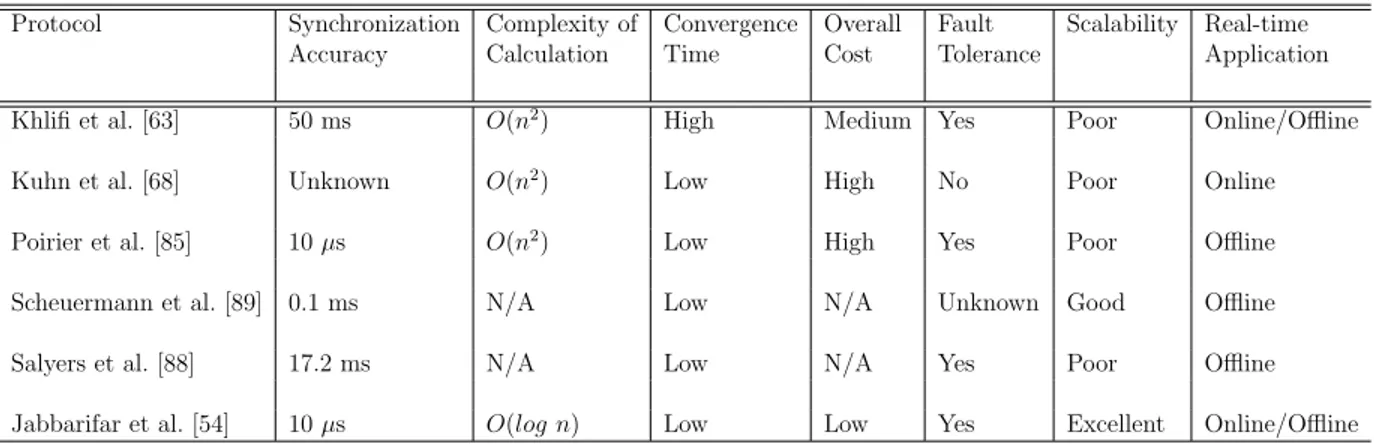
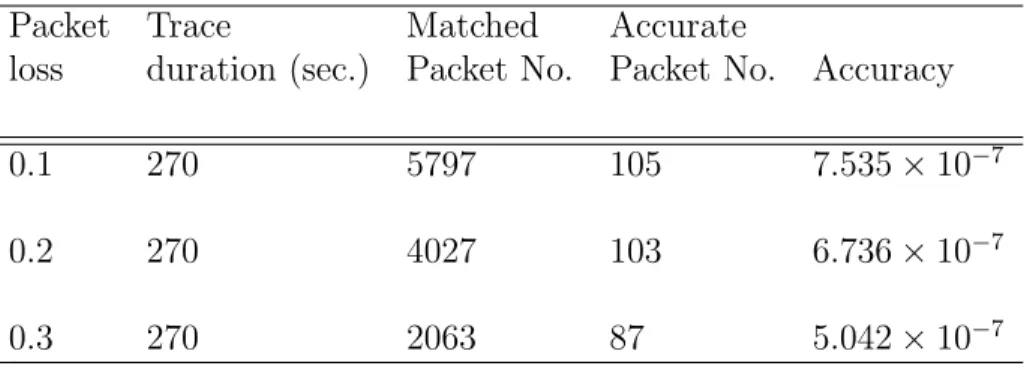
Table 2.1 Performance comparison of synchronization protocols . . . 26 Table 3.1 The packet loss affection on Fully Incremental approach . . . 58 Table 4.1 Number for each operation, from a total of one million operations . . . 79 Table 4.2 The result of proposed algorithm for six datasets in term of RN changes 80 Table 4.3 The status of join operation . . . 81 Table 4.4 Number of descendantSize update in each operation . . . 82 Table 5.1 Number of operations by type, out of a total of one million operations . 102 Table 5.2 Number of operations which affect and update the MST, out of a total

of one million operations . . . 102 Table 5.3 Dataset features and number of RN changes . . . 106 Table 5.4 Time evaluation with the Non Incremental method . . . 109 Table 5.5 The MST, RN, and conversion parameter update computation time

with the Non Incremental [85] method applied on 2-second windows . . 110 Table 5.6 Decomposition of the execution time for the proposed method . . . 113

LIST OF FIGURES

Figure 1.1 Synchronization view of LTTV . . . 3

Figure 1.2 Synchronization view of TMF . . . 5

Figure 1.3 Synchronization architecture . . . 6

Figure 2.1 SYNC message . . . 14

Figure 2.2 Convex-hull method. . . 19

Figure 3.1 Two different approaches for online synchronization. . . 37

Figure 3.2 Convex-hull method. . . 39

Figure 3.3 The local clock values used for traces T0 and T1 may be highly desyn-chronized. Two traces starting about at the same time may see start times of 600sec. and 800sec. on their local clocks, respectively. With a window size of 3sec., the first window, W1, will go from 600sec. (mi-nimum start time) to 803sec. (maximum start time plus window size). After processing the first time window, and analyzing matching events, it may be computed that trace T0 should be offset by -200sec., using T1 as time reference. The second time window, W2, is from 803sec. to 806sec., based on the reference time of T1. This corresponds to 603sec. to 606sec. in T0 based on its local clock. After synchronization, we rea-lize that events in T0 for time range W2 have already been processed as part of W1. These already read events are skipped. . . 44

Figure 3.4 Correlated sliding window. . . 46

Figure 3.5 Fully Incremental Approach . . . 47

Figure 3.6 Geometric movement state in upper and lower hulls . . . 48

Figure 3.7 The number of matched packets in each window. . . 53

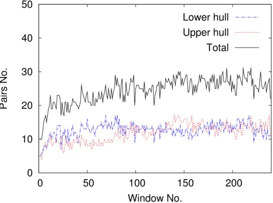
Figure 3.8 The number of pairs in Convex-Hull in each window (Correlated ap-proach). . . 53

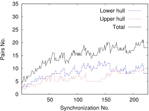
Figure 3.9 The number of pairs in Convex-Hull in each synchronization (Fully Incremental approach). . . 54

Figure 3.10 Comparison of total pairs in Convex-Hull. . . 54

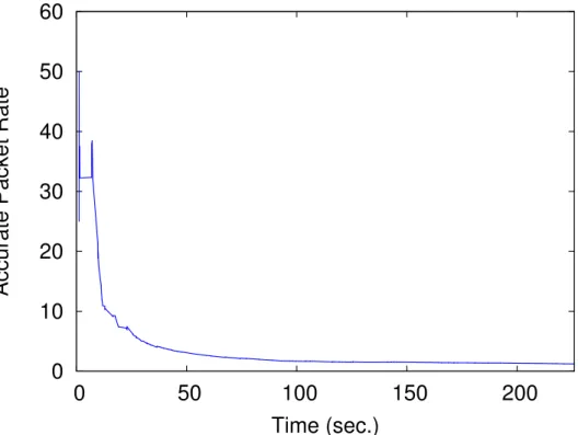
Figure 3.11 Accurate packet rate . . . 56

Figure 3.12 Accurate packet distribution vs. time window enhancement . . . 56

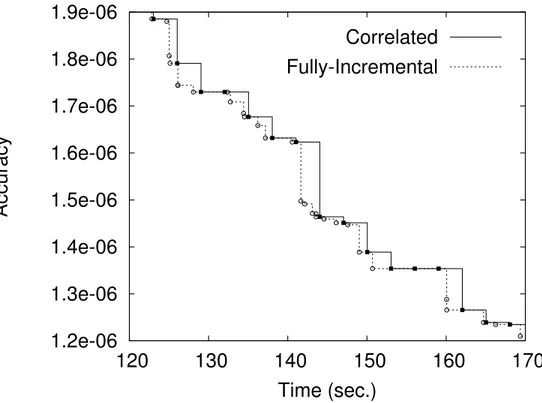
Figure 3.13 Comparison of time synchronization approaches in streaming mode. . . 59

Figure 3.14 Zoom on the accuracy dimension of Figure 3.13 from 1.2e−06 to 1.9e−06 and the trace time dimension from 120 to 170 second. . . 59

Figure 4.1 The DescendantSize operation in insertion mode with no tree cycle . . 67

Figure 4.2 The position of add() and cut() . . . 69

Figure 4.3 One way the previous reference node can remain an RN . . . 72

Figure 4.4 One case of joining two trees . . . 74

Figure 4.5 Execution time for recomputing the RN as a graph with an increasing number of updated vertices. The updating sequences contain one mil-lion operations, consisting of Insertion, Join, Cycle, and updateEdge, in a forest. The previous algorithm measured here has a complexity of O(n2) . . . 83

Figure 4.6 Dynamic Time RN : running time on a random graph with an increa-sing number of vertices plotted uincrea-sing an algorithm with a complexity of O(log n). Updating sequences contained one million operations in-cluding Insertion, Join, Cycle, and updateEdge, in a forest . . . 84

Figure 4.7 The rate of page faults with the proposed method : running time in-creases linearly with the number of nodes. . . 85

Figure 4.8 The memory usage of the proposed method ; the running time increases linearly with the number of nodes. . . 85

Figure 5.1 Convex-Hull method. . . 93

Figure 5.2 Fully Incremental Approach . . . 94

Figure 5.3 Fully Incremental Approach . . . 96

Figure 5.4 A general example of a resynchronization area when the MST changes . 100 Figure 5.5 Execution time for recomputing the MST as a graph with an increasing number of updated vertices and edges. The updating sequences contain one million operations, consisting of Insertion, Join, Cycle, and upda-teEdge, in a forest. The proposed algorithm measured here has a time complexity of O(log n) . . . 103

Figure 5.6 Dynamic Time RN : running time on a random graph with an increa-sing number of nodes plotted uincrea-sing an algorithm with a complexity of O(log n). Updating sequences contained one million operations inclu-ding Insertion, Join, Cycle, and updateEdge, in a dynamic network . . 103

Figure 5.7 Map of the computer cluster used in the experiment . . . 105

Figure 5.8 Comparison between the Fully Incremental and Non Incremental me-thods for pairwise computer time synchronization . . . 111

Figure 5.9 Comparison between the two methods for the complete network time synchronization computation . . . 112

LIST OF SIGNS AND ABBREVIATIONS

ACK Acknowledge

API Application Programming Interface BTS Branch Trace Store

CPU Central Processing Unit CTF Common Trace Format DSB Data Synchronization Barrier GPS Global Positioning Satellites ID IDentification

IBM International Business Machines I/O Input/Output

IP Internet Protocol IRQ Interrupt Request

KVM Kernel-based Virtual Machine

LIANA Live Incremental Asynchronous Network Analysis Log Logarithm

LTTng Linux Trace Toolkit Next Generation LTTV Linux Trace Toolkit Viewer

MPI Message Passing Interface MST Minimum Spanning Tree NTP Network Time Protocol

NTPD Network Time Protocol Daemon OS Operating System

PIT Programmable Interrupt Timers PTP Precision Time Protocol

QoS Quality of Service QEMU Quick EMUlator RN Reference Node

RT Real-Time

RTT Round Trip Time

SNTP Simple Network Time Protocol ST Splay Tree

SYNC Synchronization

TMF Tracing and Monitoring Framework in the Eclipse framework TSC Time Stamp Counter

UDP User Datagram Protocolor UTC Coordinated Universal Time UST User-Space Tracer

CHAPTER 1

INTRODUCTION

The arrival of multi-core processors in computer clusters represents an evolutionary change in conventional computing to obtain high performance computing. However, these systems may exhibit coherency problems when parallel programs access shared resources, thus creating hard to debug timing related problems. It is therefore crucial to have proper tools to monitor, trace and analyze system execution, in order to identify functional and performance problems. A trace facility aims to keep track of functional flow and report relevant changes at certain times. An efficient and accurate system level tracing is required to monitor and maintain distributed systems.

Over the years, different tools have been implemented to trace operating system behavior by recording kernel events. Some of the most interesting tracing tools are Ftrace [5], Dtrace [4], Systemtap [9], and LTTng [8]. The currently available trace visualization tools have often targeted detailed traces for small real-time embedded systems, or much less detailed system logs for larger systems. Moreover, existing tracing tools for distributed systems often use coarse higher level events, at the message passing programming interface layer, for which local clock differences may not be a problem ; using a time sychronization service daemon may provide sufficient accuracy in that case, to combine timestamps from several nodes as if their clocks were synchronized.

In newer distributed systems, with shorter and more frequent interactions between nodes, higher accuracy is desirable, especially for measuring and debugging low latency operations. This is the case, for example, for telecom servers, and high performance web sites such as search engines. This explains the high interest for accurate traces synchronization, providing higher accuracy and avoiding the requirement for a time synchronization service in the system under study. Indeed, a major challenge, in monitoring and debugging tools for live systems, is to minimize the impact of tracing on the traced computer.

1.1 LTTng

LTTng, developed at Ecole Polytechnique de Montreal, provides a detailed execution trace of the Linux operating system with low overhead. LTTng, like other tracers such as Perf [27], Xtrace [43], and etc.[28], uses probes to track system events. The probes fetch some information, and write it in event records. An event record contains an event identifier,

a timestamp, and optionally an event specific payload. Probes, when currently enabled, are called when the associated instrumentation is encountered during execution.

LTTng is a prime example of low overhead tracing used for measuring small intervals, for instance system call entry and exit, which may happen within one microsecond. LTTng is thus capable of handling huge traces of several gigabytes or more [29]. LTTng not only has a very low overhead but it is also able to trace kernel space and user space activities simultaneously. These specific characteristics of LTTng help monitoring an ample range of activities in a computer [8].

However, to handle huge detailed traces collected from multiple system nodes and em-bedded devices, for both online and a posteriori offline analysis and viewing, a new approach is required. Furthermore, while LTTng started as a tool for a posteriori analysis, the latest improvements now enable the live tracing and streaming of traces from multiple nodes. In a computer cluster, multiple nodes produce separate trace streams independently. Events in the traces come with a timestamp. Since timestamps are recorded based on a local clock that runs asynchronously on each node, the logical order of events cannot be guaranteed. Global trace analysis, therefore, faces the problem of converting the local timestamp values to a common reference time. Consequently, the aim of this work is to provide a new, efficient and accurate traces synchronization algorithm for live trace viewing and analysis. Indeed, LTTng should be able to visualize traces from several distributed systems on a common reference time base.

1.1.1 LTTV and TMF

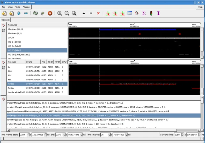
LTTV, Linux Trace Toolkit Viewer, is the stand-alone viewer for kernel and userspace traces. It is written in C/C++ using Glib and GTK+. It uses libbabeltrace to read the LTTng CTF traces. Figure 1.1 shows a screenshot of LTTV.

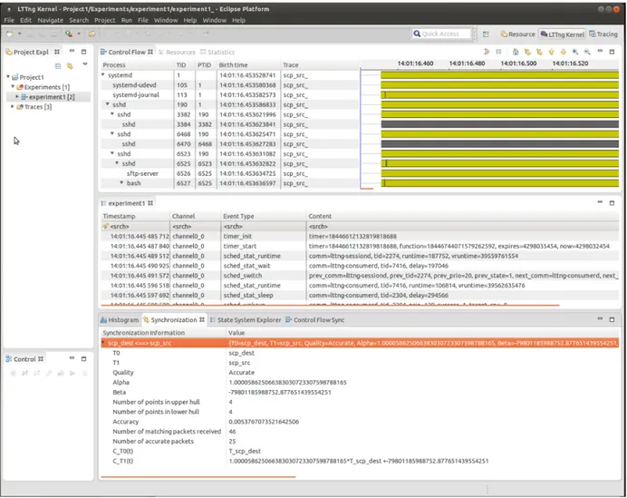
TMF, the Tracing and Monitoring Framework, is an Eclipse plug-in to view LTTng kernel and userspace traces. It is part of the Linux Tools project at Eclipse and was used to prototype the new proposed approach. TMF provides different types of detailed trace analysis. It offers different views such as the ”Control flow view” and ”Statistic view”, which facilitate trace analysis [7]. Figure 1.2 shows a screenshot of TMF where two trace files are shown with a common time base. Meanwhile, the synchronization parameters, relating each local clock to the common time reference, are shown in the synchronization view at the bottom of this Figure. Two traces with the names of scp dest and scp src are illustrated and their connection status is shown in row Quality. The Accurate label for this row indicates that the synchronization was achieved correctly at this moment. Hence, the drift and offset of these two traces are shown in the next two rows (alpha and beta) respectively. In addition, other

synchronization parameters are represented in following rows. 1.1.2 Synchronization Architecture in LTTng

Prior to the work proposed here, the synchronization of two traces in offline mode (tracing is completed and saved in a file on each computer) had been implemented recently in LTTng [85]. The main concern was to achieve a high accuracy with this trace analysis enhancement. It consisted in a post-processing step called offline synchronization [85]. This method was applied to traces recorded at the kernel level with low intrusiveness in offline mode. Figure 1.3 illustrates the general architecture of the synchronization model, showing the synchronization steps. There are four connected modules in it. Each module receives input from one or more modules and sends output to other modules.

The input of this architecture is fed by LTTng and consists of two or more unsynchronized trace files. The output is two or more synchronized traces. The output format is compatible with LTTV and TMF, which are able to show synchronized traces. The following modules are present in this architecture :

Processing module : Traces are gathered from all distributed nodes in distributed systems, and are ready to be analyzed. In order to synchronize traces from two nodes, net-work traffic exchanges between them are required. Packet exchange events are extracted and dispatched to the next module. Thus, this module captures network traffic and computer activity and extracts the necessary information for the matching module.

Matching module : Event processing feeds the events one by one. However, the Analysis module works on groups of events. Consequently, the Matching module is responsible for forming these groups. The relations between the packets are of different types (”one to one”, ”one to many”, or a mix) and this will influence the overall behavior of the module for TCP, UDP or MPI. This module must match the sent and receive events for a same packet and group them. For example, for linear regression, the round trip time (RTT) is needed, so this module makes a group after finding an acknowledgment packet, and the acknowledge time will be assumed as reference time.

Analysis module : There are two methods to synchronize time ; Linear Regression and Convex-Hull. In this module, the user can choose any of these methods to synchronize traces. The Convex-Hull method synchronizes traces with better accuracy. Consequently, it is chosen as the default option.

Reduction module : Matched packets are sent to the Analysis module without any processing and are then used to synchronize each node pair based on the Convex-Hull. The reference time is computed and all nodes can be synchronized with this reference time. Then, the reference node, the node which has the most accurate links to other nodes, is selected

Figure 1.3 Synchronization architecture

and each node pair is synchronized. However, sometimes an indirect path between two nodes has better accuracy (less drift and offset) and is chosen. To find those precise links (and drift/offset) between all node pairs, a Minimum Spanning Tree (MST) ordered by accuracy is computed. It ensures a minimal synchronization tree and the best accuracy in distributed systems. Using a spanning tree has been useful in other similar applications such as wireless sensor networks. The last part in this module is propagation. All nodes should be synchronized based on the reference node time, and drift and offset factors (α and β), propagated through the paths to the reference node. At the end, the resulting times, converted to a common reference node, become available to the user interface and trace events are shown in LTTV and TMF with right time order.

The work proposed here retains in large part this architecture but transforms each step to efficient incremental algorithms, while maintaining the same accuracy.

1.2 The Contributions of this thesis

Our goal was to achieve an incremental synchronization scheme with high accuracy and low impact. The results of this research were evaluated in the context of a tracing environ-ment, and showed excellent performance. Therefore, the presented approaches can be used for online time synchronization in computer networks even under the most demanding conditions. Our work guarantees the best accuracy, taking into account all the Convex-Hull constraints generated by matched packets as they arise, as well as optimal performance and scalability.

connected systems. As soon as two computers start exchanging messages, this method starts computing the clock offset and drift between the two, based on an optimized Convex-Hull al-gorithm. Since the Convex-Hull algorithm relies on the packets with lowest latency, it insures the best time synchronization accuracy. This method updates the synchronization factors when an accurate packet is exchanged and incrementally improves the time synchronization. This method not only does not need any buffering, but also takes O(1) time on average for updating the synchronization, when a new accurate packet is found, which is ideal for live online analysis.

Secondly, we presented a novel incremental method to compute the synchronization para-meters at the link level and maintain a Minimum Spanning Tree formed by the most accurate links. In a dynamic network, where computers connect/disconnect to/from the network, we efficiently maintain a dynamic MST. The proposed method is based on splay trees, in which every operation on the tree, such as computer connection, joining separate networks, and so on, takes O(log n) where n represents the total number of computers in the network. Therefore, instead of updating the whole MST, the network tree splays on one of updated nodes and the computation is performed upon a portion of the network.

We finally proposed a new method to select and maintain a central reference node in a dynamic network and then update the synchronization parameters. This work is performed for tracing and monitoring purposes, where a time Reference Node is required to synchronize the traces from all the nodes in a dynamic network. In the proposed technique, a novel schema analyzes new vertex insertions, tree merging, and cycle handling in a forest, minimizing average time complexity per operation in the dynamic network. What distinguishes this work from previous work is that it investigates only the altered path with respect to the Reference Node, once an alteration has occurred in the network. The proposed method incrementally processes updates in evolving trees in the forest and thus improves performance.

This new live approach to traces synchronization is fully incremental and most efficient. It not only does not degrade the accuracy of the results, but it also does not delay the syn-chronization improvement updates. Moreover, it minimizes buffering, an important feature for scaling to large computer clusters and distributed systems. We tested the proposed ap-proach on extremely large clusters, with a real network containing more than 55 physical computers, and in a simulated network containing 60,000 nodes. The results demonstrated that the proposed method addresses the accuracy, performance and scalability needs. Hence, this can be used in all cases where an efficient online time synchronization is desired.

1.3 General organization of the thesis

This dissertation is organized in seven chapters and submitted as a ”thesis by articles”. This first chapter, introduction, clarifies the context and framework of the research project. It is then followed by the body of this doctoral thesis which consists of four main articles presented in Chapters two to five. The detailed literature review is represented in a survey paper in Chapter 2 with title ”A Comprehensive Survey of Techniques and Challenges in Distributed Systems Time Synchronization”, submitted to Journal of Network and Computer Applications. This second chapter aims to bring a sufficient understanding of the issues and methods used in this research project [53]. Chapter three presents the second article entitled : “Streaming Mode Incremental Clock Synchronization”, submitted to Springer Journal : Net-work and System Management (JONS). This scientific article introduces an efficient and fully incremental, continuous time synchronization approach for links between two computers. It offers high precision and low intrusiveness for online applications and constitutes the first main original contribution [57]. The fourth chapter contains the scientific article entitled : ”Reference Node Selection in Dynamic Tree”, submitted to the Journal of Network Manage-ment. This work presents an efficient incremental method to select and update the optimum reference node in dynamic networks where nodes connect/disconnect frequently. This is used to efficiently select the time reference node in order to achieve high synchronization accu-racy, as required for real-time process-level tracing in a live distributed system. It constitutes the second main original contribution [55]. The fifth chapter presents the last article entit-led : “LIANA : Live Incremental Time Synchronization of Traces for Distributed Systems Analysis”, submitted to the Journal of Network and Computer Applications. It addresses the complete process of achieving online distributed trace synchronization in real-world live distributed system tracing. It proposes new algorithms to update the time synchronization MST, based on the link level synchronization of Chapter 3, and passes the updated MST to the incremental reference node selection algorithm of Chapter 4 [54]. A general discussion on this research area, and the results obtained, is presented in Chapter 6. This is followed in Chapter 7 by a conclusion and recommendations for future work.

CHAPTER 2

LITERATURE REVIEW : A Comprehensive Survey of Techniques and Challenges in Distributed Systems Time Synchronization

Masoume Jabbarifar and Michel Dagenais 2.1 Abstract

With the appearance of a new generation of distributed systems applications and cloud computing environments, the need arises to revisit the discussion of time synchronization. In such environments, individual physical nodes in large data centers come and go while applications and virtual machines migrate from one physical node to another. A significant problem in this context is to trace and monitor events, with a common reference time, on interacting applications and systems. Yet, tracing and monitoring tools are more important than ever to properly analyze problems in online applications under high load. Thus, time synchronization between interacting nodes is highly desirable. This paper presents a survey and classification of time synchronization protocols according to a variety of factors such as accuracy, scalability, and cost. The provided context helps designers to select the most practical synchronization protocol for their own purposes. The detailed analysis of the cha-racteristics of each approach guides developers to design and characterize new protocols with the desired feature set for a distributed system application. Furthermore, this paper presents a comparison framework through which designers can correlate and analyze the features of new and existing synchronization protocols.

2.2 Introduction

Time synchronization plays an important role for many applications in distributed systems and networks, where many nodes may interact or observe the same events. The information is collected at each individual node in the network, yet it may need to be assembled to build a coherent observation in order to achieve higher-level analysis. One of the key and fundamental ingredients for a coherent observation is a common time reference. For example, when nodes trace the actions related to a problem or a cyber-attack, then higher-level information (such as system performance analysis, attack sources and destinations) can be extracted by correlating data from multiple nodes.

Researchers have created several time synchronization protocols for wired and wireless networks over the past years. Since the challenges posed by wireless networks, such as energy efficiency and movement, are different, time synchronization in wireless sensor networks is considered a separate branch and is outside the scope of this article. On the other hand, wired network applications are growing rapidly with new applications and associated challenges appearing. In particular, online applications deployed in distributed systems require a fast and precise protocol to synchronize streaming data such as execution traces. While many applications insist on either accuracy or cost, applications such as tracing and monitoring need both at the same time. Indeed, tracing tools need to be minimally invasive to not change the system behavior under study, yet high accuracy is required to solve the most difficult problems. This is similar to electronic test and measurement equipment requiring much higher performance than the systems under test.

This paper addresses three main objectives. First, it surveys traditional clock synchro-nization protocols in distributed systems, and looks at new requirements and solutions for applications such as traces synchronization. This review is based on several factors such as accuracy, scalability, and cost, and will help designers to select the most efficient protocol for their application. Secondly, the analysis of the features, protocols and usecases of the different approaches presented should enable developers to combine or adjust existing ap-proaches for specific application goals. Finally, this paper provides a framework to present different functional aspects and comparisons of the existing synchronization approaches.

Although there are several survey papers on time synchronization, they either predate many of the new applications exposed here [37, 66, 100] or focus on specific usecases such as wireless sensor networks [10, 11, 46, 96, 99]. Wireless sensor networks have several specific concerns of their own, such as energy and movement, and form a somewhat separate branch. In this work, we rather focus on distributed systems which bring different and new usecases, such as telecommunication services, online business applications, online gaming and etc.

This paper is organized as follows. Section 2.3 presents the concepts and foundations of clocks synchronization protocols. Section 2.4 provides a classification of synchronization ap-proaches into online and offline classes. Section 2.5 contains an evaluation of several protocols and a comparison among them based on several factors, which are discussed separately. Sec-tion 2.6 lists different challenges that influence the time synchronizaSec-tion accuracy and cost. Finally, we conclude our survey paper with Section 2.7.

2.3 Clock and Synchronization Protocols

The ultimate common reference time usually is the Coordinated Universal Time (UTC ) [90]. UTC is a standard global time source provided by several governmental laboratories around the world and normally based on atomic clocks. It is available as primary time ser-vers on the Internet and as over-the-air electromagnetic signals. Another important precise common time reference is the Global Positioning Satellites (GPS ) system [71], built around a large number of satellites, each containing an atomic clock. The two time referentials dif-fer by several seconds since UTC adds leap seconds every few years to synchronize with the earth rotation, while GPS clocks simply follow their atomic clocks with no attempt to remain synchronized with terrestrial days.

While most systems ultimately synchronize with UTC, the major concern usually is to have a precise common reference time within a distributed system in order to compare related events arising on different nodes. In that context, the accuracy of the synchronization between the different nodes in the distributed system is often much more important than the accuracy of the synchronization with UTC.

The problem arises from the fact that each computer node has an independent clock. In theory, it would be possible to distribute a common clock to several computers in a data center. This could be achieved by a light source feeding several fiber optics cables with carefully measured cable lengths. Indeed, signals in either electrical wires or fiber optics travel at approximately 2/3 of the speed of light or about 6ns per meter. All cables could have the same length or compensation factors could be computed based on the cable length to each node. Then, this signal should be connected directly to the processor internal clock, a facility not available on most systems. Specialized telecommunication equipment may use similar schemes because of their stringent needs on clock synchronization for high speed protocols such as SONET [36].

A common mechanism is to have a timing signal cable providing a pulse per second signal at the beginning of each second. This cable is connected to an input signal that can generate interrupts on the node (e.g. a pin on the serial or parallel port of many computers). For example, a very precise pulse per second signal may be provided by relatively inexpensive GPS timing receivers. The main source of inaccuracy then often becomes the interrupt latency, for the computer node to be notified of the interrupt generated by the pulse per second signal [22, 33, 74].

When no such special purpose hardware is available, time synchronization is achieved through the existing network hardware. Packet exchanges between nodes can be used to estimate the clock offsets. This will be the focus of the remainder of this article. Different

strategies may be used in order to compare events on a common time reference. The most prevalent, [75], attempts to keep the clock at each node as close as possible to a reference clock, typically UTC. Then, events at each node are loosely based on the same time reference. A second approach, used for tracing, is [85] where the clock at each node does not need to be especially well synchronized. Instead, the a posteriori analysis of packet send and receive events in traces is used to deduce with high accuracy the offsets between the clocks in each node. Finally, a third approach is used when tracing information is displayed live, in quasi real time, [57]. The approaches are similar to a posteriori analysis except that the computation must be performed incrementally and that the offset estimation may improve over time as more packet send and receive events are analyzed.

2.3.1 Time Keeping Hardware

When a computer node is started, it needs to initialize its internal clock. This is usually achieved by reading the current time from a special battery-backed circuit called Real Time Clock. This circuit is typically not used thereafter during normal operation because of the delay to read from this slow peripheral. Instead, the operating system uses a regular interrupt to update its internal clock. Most processors contain at least one and often several Program-mable Interrupt Timers (PIT) that can be used for that purpose [21]. Unix and early Linux systems received interrupts to update their internal clock every 10ms. This was later changed to each 1 ms.

When a finer granularity is required, a cycle counter can often be used, such as the Time Stamp Counter (TSC ) on Intel processors. The TSC is a special hardware register incremented at each clock cycle. It thus provides a high-resolution, low-overhead, and fine-grained (about 1 nanosecond or better) time source [31]. However, if the processor frequency changes, the TSC rate will change as well on most systems. When the processor goes into idle or halted mode, the TSC may stop altogether. With the advent of multiple processor cores on a single chip or motherboard, the TSC s on different processor cores may drift away from each other over time, and there is no guarantee that they will ever resynchronize.

A new generation of multicore processors from Intel include a constant rate TSC, which provides for synchronization of the cores even though their frequency may vary over time [81]. Indeed, a constantly running clock, shared by many processor cores, is used to update these TSCs [64]. The TSC can then be used as the only time source for kernel and user space needs.

The interaction between these multiple clock sources can be problematic. Linux systems have a system clock tracking UTC, typically through the Network Time Protocol. Howe-ver, the time adjustments can distort time measurements needed by the operating system,

for instance in device drivers. While it is not recommended, the system clock may even be adjusted to go back in time. For this reason, another clock source is defined in the kernel, CLOCK MONOTONIC, which is never adjusted during the execution and progresses regard-less of UTC. It represents the absolute elapsed time since an arbitrary point. It keeps increa-sing and is synchronized between all processor cores in a node [26]. It may run slightly faster or slower than real time, its rate may vary slightly due to environmental conditions like tempera-ture or voltage, and it may jump ahead when in a virtual machine and coming back from being scheduled out. This clock source is typically built from the regular timer interrupts at every milisecond, with the TSC being used on Intel processors to interpolate between two timer interrupts and provide the needed high resolution. The time update at each timer interrupt is synchronized among the multiple processor cores, enabling the CLOCK MONOTONIC to be fairly well synchronized between cores. CLOCK MONOTONIC is used in the LTTng tracer [8], insuring a high resolution common reference time among the processor cores on a single node [20, 62, 84].

2.3.2 Packet-based Clock Offset Calculation

When a packet is sent from time server node S to client node C, C ’s clock could be set to S ’s clock plus the delay for the packet to travel between the two nodes. The problem with this simplistic approach is that the nominal network delay may not be known. Moreover, network congestion or operating system latency may delay almost indefinitely the delivery of the packet to the clock synchronization application.

A better approach was proposed by Cristian [25]. This method is based on the round-trip time (RTT ) between a computer C and a time server S. C sends a time request to S. Once S receives the request, it responds by appending its current time TS to the message. Then,

C calculates the time with Formula 2.1 and updates its clock accordingly. This technique assumes that the network delay is the same for the request and the response. When this is the case, perfect accuracy is obtained. Otherwise, the computed time value is within ±RT T /2 of the real value. To improve the accuracy, C can send multiple requests to S and retain the response with the smallest round-trip time (RTT ).

TC = TS+ (RT T /2) (2.1)

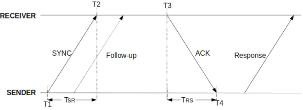
This was further improved upon by incorporating into the equation the processing time of the server. Unlike the network delay, this processing time, albeit small, is easily obtained. Figure 2.1 illustrates that the sender issues to the receiver a message at T1. The receiver notes T2 as the reception time. Then, the receiver returns an ACK message to the sender

at time T3. The sender receives the ACK message with T4 as reception time. Finally, at the end of the message exchange, the sender can compute the offset and accuracy from the four timestamps embedded in the Response message with Formula 2.2. The sender adjusts its clock according to the offset and the synchronization is performed.

Here again, the method assumes that the sender-receiver and receiver-sender propagation times are exactly equal, in which case perfect accuracy is obtained. Otherwise, the bound on accuracy is provided. Since the inaccuracy is related to the time elapsed between T1 and T2, and between T3 and T4, one optimization is to get these time values as close as possible to the packet send and receive points in the kernel. For example, in the LTTng tracer, which uses this technique to synchronize traces, the packet send and receive events in the trace are generated in the kernel at the lowest possible point in the network stack, just ahead of the interface with the NIC driver [85]. The values of timestamps are thus obtained much closer to the packet send and receive points. This is used in order to obtain a better accuracy than what can be achieved when generating timestamps at the application level in a time synchronization daemon. Another interesting aspect of LTTng is that the information from existing packets is used to compute the offset, keeping the tracer minimally invasive since it is not necessary to send additional packets for time synchronization.

This synchronization method, based on Equation 2.2, is the basis for the Network Time Protocol (NTP ), a standard Internet protocol for clock synchronization. It proposes an or-ganisation with two levels of time servers : Primary and Secondary time servers. A primary time server synchronizes directly with a reference time source, usually a UTC atomic clock. Secondary time servers synchronize with primary time servers or other secondary servers. A client typically synchronizes with its nearest secondary time server. NTP, depending on the network latencies, typically achieves an accuracy between one and ten milliseconds in local networks and tens or even hundreds of milliseconds in wide area Internet. The Simple

Network Time Protocol (SNTP ) is a simplified version of NTP for users [80]. Of f set = [(T 2 − T 1) + (T 3 − T 4)]/2

Accuracy = ±[(T 2 − T 1) − (T 3 − T 4)]/2

(2.2)

The Precision Time Protocol (PTP ) [38] uses the same equation to estimate the network delay between each node and the time server. However, hardware support in the networking equipment can be used to insert the reference time at the network switch level in a broadcast packet, insuring that all clients receive the reference time in parallel and with a very short network delay. Furthermore, networking equipment is optimized to minimize network delay variations and asymmetry. As a result, PTP can achieve clock synchronization accuracy at the microsecond level.

When no time server is available, several computer nodes can communicate their clock values and compute an hopefully more precise average value as the reference. This is the main idea behing the Berkeley protocol [24, 66, 100].

2.3.3 Logical clock Synchronization

Some applications only require causal ordering of events. Hence, they use logical clocks to order events. Each pair of related events is ordered by causality relations (such as the send event for a packet necessarily happening before the receive event). This type of syn-chronization is called logical time. Lamport proposed algorithms to compose logical clocks. The limitation of his algorithm is that it cannot necessarily specify which one is executed first when timestampe1 < timestampe2, unless they refer to the same logical clock [65, 69].

Mattern and Fidge proposed a method based on Vector Clocks to address this problem and determine precedence. Landes et al. use a tree structure to improve Vector Clocks limitation. However, the storage and message size increase with the number of nodes [70]. Logical clocks suffer from two important limitations. First, they cannot provide precedence relationships for events without explicit causality relationships, for example two computer nodes interacting with the same shared storage device (thus indirectly but not directly interacting). Secondly, there is no notion of absolute time, which is important in several applications.

2.4 Synchronization techniques to compute clock offset and drift

As seen in the previous section, network packets sent among nodes are used to compute the clock offset between communicating nodes. Packets may be sent explicitly for time syn-chronization, carrying the send and receive time values for the exchange, or a trace of ordinary

packets sent and received at each node can be taken and sent later to an analysis node. In either case, it is interesting to combine the information from several packet exchanges to get a more precise estimate of the offset, and its variation over time. The exact frequency of the clock at a node can vary somewhat. Several computers with a 2 GHz nominal frequency will in practice all have a slightly different frequency. That frequency, for a given node, is however extremely stable over a time as long as factors such as the operating temperature or the supply voltage do not vary significantly [75]. For this reason, the clock offset between two nodes varies linearly with time as a factor of the ratio of their respective frequency. It will therefore be represented as a linear function with the initial offset and drift as coefficients. The two main methods to estimate this linear function, based on the data from several packet exchanges, are the Linear Regression and the Convex-Hull.

Linear Regression

The Linear Regression models a response variable, y, as a linear function of a single predictor variable, x. The formula for this definition is : y = a × x + b, where “a” and “b” are the regression coefficients. Coefficient “a” is the slope of the line and “b” defines the Y-intercept. In our case, “a” is the clock drift, “x” is the time and “b” is the initial offset.

In a two dimensional space, based on timestamps of node A and B, the Linear Regression algorithm tries to fit a line among the points. Packet A sent from node A has a timestamp that provides the x coordinate. As soon as it is received in node B, its timestamp is obtained and becomes the y coordinate. These two coordinates define a point in the two dimensional space. Since there are many packet exchanges in a regular connection, many points will be obtained in this way [95]. It is obvious that a line can be drawn through two points. However, there are typically many more than two points and just one line should model the whole information. The solution is based on the method of least squares. This model estimates the best-fitting line that minimizes the differences with actual data. If each point in the two dimensional space is represented by its x and y values, and there are N points (total number of exchanged packets), the average of x and y values are obtained as shown in Formula 2.3.

x = Σni=1xi

n

y = Σni=1yi

n

(2.3) Both regression coefficients are estimated with Formulas 2.4 and 2.5.

a = Σni=1(xi−x)×(yi−y)

Σn

b = y − a × x (2.5) In these equations, “a” and “b” are the drift and offset respectively between the two clocks. While the linear regression gives adequate results, there are significant weaknesses with this approach. The first is that the measurement error is biased. When everything works as expected, a minimal delay is achieved and a very good point is obtained. The system and network delay cannot go under this minimum, corresponding to the ideal case. However, if the system is preempted by a high priority interrupt or there is network congestion, a much longer delay may be obtained creating a bad point. The problem is that the linear regression takes into account all points when calculating the best fit. To alleviate this problem, some have proposed to detect and eliminate outliers, not using them for the linear regression [22] and obtaining more precise results. A second problem is that the x and y values, the time at nodes A and B, are not sampled simultaneously ; they are separated by the packet propagation time. However, if the number of packets, used for the linear regression, is the same in each direction, the errors in each direction should mostly compensate for one another.

Convex-Hull

The Convex-Hull algorithm is based on the fact that each packet implies that the receiving time is later than the sending time. Thus, it does not suffer from outliers since they bring weaker constraints which have no effect on the result. Similarly, the fact that there is a network delay between the time at which x and y are measured does not contradict the inequality indicating that the receiving time (even with the network delay added) is after the sending time.

As shown in Figure 2.2, pairs are divided into two sets, based on the message direction. Consequently, the synchronization estimation line should be below all the pairs {−(θ−−−−S_i, ξ→_iR), −−−−−−−→

(θ_i+1S , ξ_i+1R ), ...} and above all pairs {(θ←−−−−_jR, ξ_jS−),←−−−−−−(θ_j+R , ξ_j+1S ), ...}.

The packets with minimum latency are those of interest in the Convex-Hull synchroni-zation algorithm. Packets sent from θ (horizontal axis) to ξ (vertical axis) occupy the upper left half-plane and are shifted higher when more network latency was encountered. There-fore, the lower half-hull, of the Convex-Hull formed by those points, is a lower bound for the packets sent from θ and identifies the packets with the lowest latency. Similarly, packets sent from ξ (vertical axis) to θ (horizontal axis) occupy the lower right half-plane and are shifted to the right when more network latency was encountered. Therefore, the upper half-hull, of the Convex-Hull formed by those points, is an upper bound for the packets sent from ξ and identifies the packets with the lowest latency. The possible synchronization lines lie below the

lower half-hull of packets sent from θ and above the upper half-hull of packets sent from ξ. The synchronization accuracy is limited by the delay between the send and receive events. Any packet delayed by interrupts, network switch delay, or some other cause will lead to an inaccurate pair and a long delay. The Convex-Hull algorithm selects the pairs on the inside envelope between the send time and the receive time, and so identifies the most accurate pairs with the shortest delay. In other words, it finds the area that has minimum latency and ignores outlying pairs, as shown in Figure 2.2 (−(θ−−−−S →

2, ξ2R), −−−−−→ (θS 5, ξ5R), ←−−−−− (θR 2, ξ2S), ←−−−−− (θR 3, ξ3S)). Therefore,

the estimated line is more accurate than with Linear Regression, not being affected by outliers. According to the above definition, we have two completely separate sets. Otherwise, this would imply a message inversion (receive before send). In each set, the optimal separator is computed (the solid line in each hull) from the points in each set nearest to the separator space. Graham’s scan algorithm selects the points forming the Convex-hull in these two separated sets. The bounds of the Convex-hull, shown in Figure 2.2, are :

U pperBound = {←(θ−−−−R − 1, ξ1S), ←−−−−− (θR 4, ξ4S), ←−−−−− (θR 5, ξ5S)} LowerBound = {−(θ−−−−S → 1, ξ1R), −−−−−→ (θS 3, ξ3R), −−−−−→ (θS 4, ξ4R), −−−−−→ (θS 6, ξ6R)} (2.6) Thus, the maximum likelihood estimators are between the following conditions :

αθS i + β < ξiR αξR j + β < θSj i, j = 1, 2, ..., n (2.7)

The next step is to find two lines, one with maximum slope (Lmax) and another with

minimum slope (Lmin) :

Lmax= αmaxθ + βmin

Lmin = αminθ + βmax

(2.8) As a result, the final estimated α and β are certainly limited to the area that is enclosed between (αmin, αmax) and (βmin, βmax), and the selected synchronization line is the bisector

of Lmax and Lmin.

When synchronizing two traces, the relationship between them can be one of the following : Definition 1) An accurate relationship : this is the expected case, shown in Figure 2.2, where Lmax and Lmin are available and their middle can be computed. If the relationship

between two clocks is of the accurate type, we can define the accuracy metric as the difference between the minimum and maximum possible drifts between the two clocks.

tξ t_θ (θR₁,ξS₁) (θR₂,ξS₂) (θR₃,ξS₃) (θR₄,ξS₄) (θR₅,ξS₅) (θS₁,ξR₁) (θS₂,ξR₂) (θ S 3,ξR3) (θS₄,ξR₄) (θS₅,ξR₅) (θS₆,ξR₆) Lmax L_min C_ξ(t_θ) β_max β_min

Figure 2.2 Convex-hull method.

Definition 2) An approximate relationship : Lmax and Lmin are not available because

the hulls do not satisfy the hypothesis that the upper half-hull should be below the lower half-hull and not intersect with it. This may be caused by a deviation from the assumed constant clock frequency, causing a higher-order (e.g. quadratic) relation between the two clocks. Other possible causes include a problem with the time measurement computation. In that case, the approximation is a ”best effort”.

Definition 3) An incomplete relationship : only one of the Lmax and Lmin lines is

available. There is communication in only one direction, which is insufficient to obtain a proper bounded synchronization.

Definition 4) An absent relationship : there is no communication between the nodes in either direction, and nothing can be deduced about their relative time.

Definition 5) Fail relationship : none of the Lmax and Lmin lines is available. This is

because the hulls completely intersect each other or are reversed.

Based on each of these definitions, two nodes either are synchronized, not synchronized, or partially synchronized. When there is no connection between two nodes, it may be pos-sible to compute their offset and dritf indirectly through other nodes with which both are communicating.

2.5 Synchronization Applications

In traditional clock synchronization, the aim is to adjust the clock offset immediately with respect to a time server [73, 77, 78]. Information from successive synchronization points is used to compute the clock drift, better correlate these synchronization points over a long period of time, filtering out less accurate values, and improving the accuracy between syn-chronization points using a correction factor. The other form of time synsyn-chronization is traces synchronization [34, 83, 86]. In that context, traces from several distributed nodes are brought together on an analysis node. The basic algorithms for synchronization remain the same but several constraints are different and the algorithms can be adapted and optimized accor-dingly. For instance, it can select the best path to compute the clock differences between two nodes among several indirect paths. Moreover, the most interesting node to use as time reference can be selected dynamically. Finally, in some cases, the trace analysis is only perfor-med offline at the end of data collection. In that case, the clock differences can be optimally computed based on the complete data set.

In this section, we will therefore examine the specificities of traces synchronization and in particular offline A posteriori Trace Synchronization and live streaming Online Trace Synchronization.

2.5.1 Offline Clock Synchronization

Recently, many time synchronization algorithms have been suggested. The main goal of these algorithms is to increase the time synchronization accuracy. All algorithms tried to estimate a function that models the time on the clock of a computer versus the time on the clock of another computer, and then propagate the estimation to other computers in a cluster.

When a message is exchanged between a pair of nodes, the receiving and sending times will not be directly comparable because the clocks of two nodes are not synchronized [12, 64, 72]. However, by the principle of causality, the receive time must be later that the send time. This constraint is used to compute the clock drift between two nodes [25].

An interesting offline clock synchronization method has been proposed by Duda et al. [37], which consists of two synchronization algorithms, Linear Regression and Convex-Hull. These algorithms estimate a conversion function between the clocks in a pair of nodes. In both algorithms, the conversion function is linear, and the drift and offset between the two clocks are extracted from this linear model [58].

It is also used to estimate the one-way delay between two nodes by Moon et al. [82]. In a two-dimensional space, based on the time values at nodes A and B, the Linear Regression

algorithm attempts to map all points to a line. Thus, every point will affect the position of that line. In reality, network latency and similar events between two nodes can cause problematic outlying points, biased being only late. These outliers should ideally not affect the drift or offset computed from the Linear Regression. They should, in fact, be ignored in order to increase accuracy [14].

The Convex-Hull algorithm does not suffer from this problem and insures the highest synchronization accuracy [59]. The Convex-Hull is a precise algorithm that assumes upper and lower bounds (sending time and receiving time) separated by the network delay. In this way, it finds the area that has minimum latency and ignores outlying points. As a result, the estimated line is more accurate with this algorithm than with Linear Regression.

Among these two algorithms, Linear Regression and Convex-Hull, the Linear Regression algorithm can use existing functions from a statistical package and is thus easier to imple-ment. However, the Convex-Hull algorithm can model clocks with higher accuracy while still requiring a modest computational complexity. The following two subsections provide more details about using each of these two algorithms.

Khlifi et al. [63] proposed two algorithms, which they call the average and direct skew removal techniques for offline skew removal. The average algorithm calculates the average delay for a fixed number of consecutive packets at the beginning and the end of a trace, yielding a constant O(1) complexity. The direct skew removal technique has the interesting property of being able to account for low clock resolution, where the clock granularity may be larger (e.g. 1ms) than the packet delay. For this purpose, the whole trace is analyzed for a linear O(n) complexity.

Clement et al. [22] have evaluated the impact of system characteristics on trace synchro-nization accuracy. First, they studied the tracing duration impact. They propose dividing long duration traces into 30 minute segments, since the error in the clock drift linear ap-proximation begins to increase significantly after approximately 45 minutes of tracing, while it is quite stable during the first 30 minutes. The error increases because of the variation in the clock drift with time, as shown by the Allan deviation [2], and because of environmental effects on the clock circuit frequency, such as temperature and supply voltage variations.

Then, they studied the impact of the system load parameter, when there is a heavy load on major subsystems, CPU, memory, and hard disk. They found that the transmission time and response time measurement variations, caused by interrupt latency in a loaded system, influence the clock drift computation directly, and subsequently the time synchronization accuracy. The third parameter studied was hop count, when there is more than one path between two nodes. In that case, the offset between the two indirectly linked nodes may be computed by adding the offsets along a path, from one intermediate hop to the next. A path

with fewer hops generally provides higher accuracy. If there is a direct path, it is normally better to choose that one to synchronize two nodes.

Poirier et al. [85] presented an accurate method for synchronizing distributed traces. This method is applied to traces recorded at the kernel level with low intrusiveness. They applied the Convex-Hull algorithm to the clocks of traced nodes as a conversion function. If collected traces are huge and involve numerous nodes, their method is time consuming. Since their algorithm was designed for post-processing, the analysis delay was not major concern. However, for a live display of traces, the latency should be minimized. In [56], the proposed method estimates accurate paths in large computer clusters and improves the performance of offline distributed trace synchronization.

2.5.2 Online Clock Synchronization

Online synchronization works in streaming mode. Several researchers have proposed algo-rithms for this application. The standard clock synchronization method, widely used today, are the Network Time Protocol (NTP) [79] and NTP Daemon (NTPD) [80]. It sets and maintains the kernel system clock, used to measure packet send and receive time, based on feedback from exchanges with the server. Veitch et al. and Ridoux et al. [87, 102] proposed the RAD clock (Robust Absolute and Difference Clock), which provides alternative clock synchronization algorithms. The timing packets are timestamped using raw packet times-tamps. They estimate the clock skew based on the difference between the system clock and the timestamps received from the server, and maintain the clock skew correction without changing the raw system clock, in a feed-forward approach.

Khlifi et al. [63] presented two techniques for online skew estimation and removal. The first one, sliding window, monitors the minimum delays to reduce the gap between the true and the corrected delays, (the correction being the estimated skew). To improve the accuracy, they present a second technique, the combined approach. They perform the sliding window algorithm to quickly estimate the skew, in the first interval. Then, they use the Convex-Hull algorithm during subsequent intervals to improve the accuracy.

A particularly efficient algorithm is proposed in [57], which is based on Converx-Hull algorithm combined with lines with minimum and maximum possible slopes between the hulls. This can provide skew estimates very early, obviating the need for a different method in the first interval. Furthermore, the proposed algorithm can identify accurate packets (those few that can improve the estimate) with a simple test and recomputes the drift and offset incrementally in O(1) upon identifying an accurate packet.