HAL Id: hal-00329371
https://hal.archives-ouvertes.fr/hal-00329371
Submitted on 7 Sep 2004
HAL is a multi-disciplinary open access
archive for the deposit and dissemination of
sci-entific research documents, whether they are
pub-lished or not. The documents may come from
teaching and research institutions in France or
abroad, or from public or private research centers.
L’archive ouverte pluridisciplinaire HAL, est
destinée au dépôt et à la diffusion de documents
scientifiques de niveau recherche, publiés ou non,
émanant des établissements d’enseignement et de
recherche français ou étrangers, des laboratoires
publics ou privés.
Cluster survey of the high-altitude cusp properties: a
three-year statistical study
B. Lavraud, A. Fedorov, E. Budnik, A. Grigoriev, P. J. Cargill, M. W.
Dunlop, H. Rème, I. Dandouras, A. Balogh
To cite this version:
B. Lavraud, A. Fedorov, E. Budnik, A. Grigoriev, P. J. Cargill, et al.. Cluster survey of the
high-altitude cusp properties: a three-year statistical study. Annales Geophysicae, European Geosciences
Union, 2004, 22 (8), pp.3009-3019. �hal-00329371�
Annales Geophysicae (2004) 22: 3009–3019 SRef-ID: 1432-0576/ag/2004-22-3009 © European Geosciences Union 2004
Annales
Geophysicae
Cluster survey of the high-altitude cusp properties: a three-year
statistical study
B. Lavraud1,*, A. Fedorov1, E. Budnik1, A. Grigoriev2, P. J. Cargill3, M. W. Dunlop4, H. R`eme1, I. Dandouras1, and A. Balogh3
1Centre d’Etude Spatiale des Rayonnements, 9 ave du Colonel Roche, 31028 Toulouse Cedex 4,Toulouse, France 2Swedish Institute of Space Physics, Box 812, SE-981 28 Kiruna, Sweden
3Imperial College, South Kensington campus, London SW7 2AZ, UK 4Rutherford Appleton Laboratory, Chilton, Didcot OX11 0QX, UK
*now at: Space and atmospheric sciences, Los Alamos National Laboratory, New Mexico, NM 87545, USA
Received: 18 November 2003 – Revised: 1 April 2004 – Accepted: 21 April 2004 – Published: 7 September 2004
Abstract. The global characteristics of the high-altitude cusp and its surrounding regions are investigated using a three-year statistical survey based on data obtained by the Cluster spacecraft. The analysis involves an elaborate orbit-sampling methodology that uses a model field and takes into account the actual solar wind conditions and level of geomagnetic activity. The spatial distribution of the magnetic field and various plasma parameters in the vicinity of the low mag-netic field exterior cusp are determined and it is found that: 1) The magnetic field distribution shows the presence of an intermediate region between the magnetosheath and the mag-netosphere: the exterior cusp, 2) This region is characterized by the presence of dense plasma of magnetosheath origin; a comparison with the Tsyganenko (1996) magnetic field model shows that it is diamagnetic in nature, 3) The spa-tial distributions show that three distinct boundaries with the lobes, the dayside plasma sheet and the magnetosheath sur-round the exterior cusp, 4) The external boundary with the magnetosheath has a sharp bulk velocity gradient, as well as a density decrease and temperature increase as one goes from the magnetosheath to the exterior cusp, 5) While the two in-ner boundaries form a funnel, the external boundary shows no clear indentation, 6) The plasma and magnetic pressure distributions suggest that the exterior cusp is in equilibrium with its surroundings in a statistical sense, and 7) A prelimi-nary analysis of the bulk flow distributions suggests that the exterior cusp is stagnant under northward IMF conditions but convective under southward IMF conditions.
Key words. Magnetosphere physics (Magnetopause, cusp, and boundary layers; Solar wind-magnetosphere interac-tions; Magnetospheric configuration and dynamics)
Correspondence to: B. Lavraud
1 Introduction
Extensive studies of the low- and mid-altitude cusp regions of the magnetosphere have been made using data from many spacecraft (Newell and Meng, 1988; Newell et al., 1989; Escoubet et al., 1992; Lockwood and Smith, 1992; Woch and Lundin, 1992; Newell and Meng, 1994; Yamauchi et al., 1996). However, statistical studies of the high-altitude cusp region (above 6 RE) have been more limited, and mostly
fo-cused on the high-latitude magnetopause position.
Zhou and Russell (1997) used Hawkeye spacecraft data to study the position of the high-latitude magnetopause. Based on 148 high-altitude passes they concluded that the mag-netopause at cusp latitudes is not indented, thus contra-dicting the earlier works of Spreiter and Summers (1967), Paschmann et al. (1976) and Haerendel et al. (1978).
Using HEOS-2 data, Dunlop et al. (2000) compared the observed high-altitude cusp magnetic field configuration with that from a model field (Tsyganenko, 1989). The de-viation between the two configurations (spacecraft data and model) led them to conclude that there is the presence of an indentation at the magnetopause in this region. However, they did not give reasons for their inconsistency with the re-sults of Zhou and Russell (1997).
Fung et al. (1997), and later Eastman et al. (2000), have analyzed a large number (1757 for the latter) of passes of Hawkeye in the distant cusp region. Defining the magne-topause by a complete set of criterion (overall comparable to the Dunlop et al. (2000) ones) they also concluded that the magnetopause was indented in this region. They noted the differences with the results of Zhou and Russell (1997) and suggested it may have arisen from a different magnetopause identification routine.
The generic properties of the high-altitude cusp were fur-ther investigated by Zhou et al. (1999; 2000) and Tsyga-nenko and Russell (1999) on the basis of Polar data. Zhou et al. (1999; 2000) mainly studied the cusp location as a
3010 B. Lavraud et al.: Cluster survey of the high-altitude cusp properties function of the solar wind conditions while Tsyganenko and
Russell (1999) focused on the extent of the cusp diamagnetic cavity as a function of the dipole tilt angle and IMF condi-tions. Because the Polar orbit has an apogee of 9 RE, they
did not investigate the position of the outer boundaries of the cusp region.
Grigoriev et al. (1999) also attempted to perform a statisti-cal survey of Interball-Tail passes of the region near the high-latitude magnetopause. A significant diamagnetic effect in the vicinity of the high-altitude cusp and plasma mantle was found. However, the Interball-Tail orbit declination did not allow coverage of the central part of the high-altitude cusp.
More recently, M˘erka et al. (2002) investigated the lo-cation and spatial extent of the cusp-like plasma regions observed by the Magion-4 satellite (part of the Interball mission). For this purpose they used the mid- and high-altitude Magion-4 measurements, which they mapped to low-altitudes using the Tsyganenko (1996) model with the actual solar-wind conditions. This study confirmed the cusp lati-tudinal displacement observed for varying IMF conditions, which illustrate the need to take this into account in the present paper.
The Cluster orbit permits a full examination of the char-acteristics of the high-altitude cusp and of its surrounding boundaries. We use the Cluster data to address the following objectives:
– a survey of the global magnetic field and plasma prop-erties of the cusp diamagnetic cavity (hereafter referred to as “exterior cusp”),
– the identification and characterization of the various boundaries surrounding the exterior cusp region, – a preliminary characterization of the plasma flows in
this region, and their dependence on the IMF orienta-tions.
The sampling technique used here (superposed epoch analysis) was first introduced by Grigoriev et al. (1999) and is described in Sect. 2. It allows an accurate estimation of the position of the cusp boundaries, as well as a description of its various internal features. In this paper we provide spa-tial distributions of many key plasma parameters (magnetic field, density, temperature and velocity) which give new in-sights into the overall structure of the high-altitude cusp.
Section 2 presents the sampling methodology that is used to order the data and make the spatial distributions. The re-sults and their discussion are given in Sect. 3. Conclusions are finally drawn in Sect. 4.
2 Instrumentation and methodology 2.1 Orbits and instrumentation
The Cluster spacecraft fly through the high-altitude cusp dur-ing sprdur-ing each year and the passes used here were all taken from between January and April. During 2001 and 2002, the
inter-spacecraft separation was of the order of 600 km and 100 km, respectively. Consequently, only data from space-craft 3 are used for these periods. However, in 2003 the inter-spacecraft separation was about ∼1 REand so data from both
spacecraft 1 and 3 are used.
In the present survey, we make use of the Cluster ion and magnetic field data from the Cluster Ion Spectrome-try (CIS) (R`eme et al., 2001) and FluxGate Magnetometer (FGM) (Balogh et al., 2001) instruments, respectively. The ion data come from the Hot Ion Analyser (HIA) which al-lows measurements of the full 3-D ion distribution functions and moments up to a resolution of ∼4 s (spin). However, due to the sampling method, the data are averaged as described in the next sections.
2.2 Coordinates transformations
As discussed earlier, a number of statistical studies of the high-altitude cusp region have previously been presented (Fung et al., 1997; Zhou and Russell, 1997; Zhou et al., 1999; 2000; Eastman et al., 2000; Dunlop et al., 2000). While these earlier works made use of simple coordinates systems (such as GSE, GSM or SM) to order their data spatially, here we utilize a more elaborate technique that takes into account the actual solar wind (interplanetary magnetic field (IMF) and dynamic pressure (Pram) as monitored by ACE) and
geo-magnetic (Dst) conditions during each orbit.
We use the Tsyganenko (1995, 1996) (T96) magnetic field model and the Shue et al. (1997) magnetopause model to es-timate, respectively, the displacement of the latitudinal cusp location and the magnetopause radial location as a function of the solar wind and magnetospheric conditions. In turn, this should allow us to fix more accurately the location of the various dayside boundaries in our statistics. Each orbit is sampled at intervals of two minutes; the coordinate transfor-mations that are performed can be listed as follows:
– Firstly, each orbit point A (in SM coordinates) is trans-formed into point A’ through a rotation about the XSM
axis. The rotation angle is chosen so that the orbit points are brought back into the (X,Z)SM plane, as shown in
Fig. 1a. The resulting upward axis is thus a radius; this plane is called (X,R)N orm.
– We use the T96 magnetic field model to define a ref-erence frame (coordinate system and model magnetic field) for some reference conditions; these reference conditions are defined as: IMF B=(0.0; 2.0; −0.1) nT,
Pram=2.5 nPa and Dst =−10.0 nT (a reference dipole
tilt angle was also chosen). These dynamic pressure and
Dstvalues were chosen because they constitute typical values for the solar wind and magnetosphere. We chose a mainly duskward IMF in order to avoid referencing the data set to the specific cases of northward or south-ward IMF. It is known that the cusp is displaced equator-ward (poleequator-ward) for southequator-ward (northequator-ward) IMF direc-tion (Newell et al., 1989); this duskward orientadirec-tion is median and therefore more convenient as a reference.
B. Lavraud et al.: Cluster survey of the high-altitude cusp properties 3011
Figure 1. Representation of the various coordinate transformations: (a) rotation of all orbit points about the XSM axis,
which results in a projection into the (X,Z)SM plane, (b) rotation about the YSM axis as defined by the “current”
separatrix angle (see text) by use of the T96 magnetic field model et (c) radial scaling of the orbit points as a function of the reference magnetopause position for the actual solar wind conditions (model from Shue et al. (1997)).
Fig. 1. Representation of the various coordinate transformations: (a) rotation of all orbit points about the XSM axis, which results in a
projection into the (X,Z)SM plane, (b) rotation about the YSM axis as defined by the difference between the “current” and “reference”
separatrices angles (see text) by use of the T96 magnetic field model (c) radial scaling of the orbit points as a function of the difference between the “current” and “reference” magnetopause position (model from Shue et al., 1997).
For these reference conditions in the T96 model, we search for the angle of the separatrix between the last field line that is bended (or draped) toward the dayside and the first field line that extends tailward. This angle is used as the reference angle of the reference separatrix (labeled in Fig. 1b).
– Each orbit point A’ is then transformed as follows. The actual lagged solar wind conditions and geomagnetic activity are fed into the T96 model. A specific separa-trix angle between the dayside and nightside field lines is defined for these conditions (the “current” separatrix in Fig. 1b). A rotation about the YSM axis is then
ac-complished which allows a normalization of the orbit point to the reference frame. The resulting orbit point is A” (Fig. 1b).
– Finally, a radial adjustment is performed. Using the Shue et al. (1997) magnetopause model, we define a reference magnetopause location for the reference
con-ditions given above. We then proportionally scale the point A” as a function of the radial distance difference between this reference magnetopause and the one ob-tained with the actual condition for each orbit point. This scaling is illustrated in Fig. 1c and the final orbit point is named A”’.
These coordinate transformations are applied to all the Clus-ter orbits for which both FGM and CIS (as well as ACE) data are available. This then allows us to represent the data as spatial distributions in the normalized (X,R)N ormplane.
2.3 Orbit and data sampling
As already mentioned, the Cluster orbits are sampled at in-tervals of two minutes. Cluster measurements are therefore averaged over these two-minute intervals in our statistics. The interplanetary conditions are averaged over intervals of 10 min. Therefore, these latter values are used for five suc-cessive orbit samples in order to derive the normalized orbit
3012 B. Lavraud et al.: Cluster survey of the high-altitude cusp properties
18
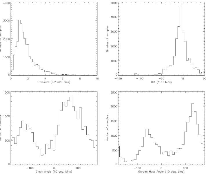
Figure 2. The distributions of the solar wind and geomagnetic parameters used in the survey. The distribution of the dynamic pressure is displayed on the top left-hand side plot, where averages over 0.2 nPa bins were used. The distribution of the DST is shown in the top right-hand plot, with averages made over 5 nT bins. The distributions of the IMF clock angle (atan-1(By/Bz)) and garden hose angle (atan-1(By/Bx)) are respectively given on the left and right-hand side plots shown at the bottom (averages were here made for 10° bins).
Fig. 2. The distributions of the solar wind and geomagnetic parameters used in the survey. The distribution of the dynamic pressure is displayed on the top left-hand side plot, where averages over 0.2 nPa bins were used. The distribution of the Dst is shown in the top right-hand plot, with averages made over 5 nT bins. The distributions of the IMF clock angle (tan−1(By/Bz))and garden hose angle
(tan−1(By/Bx))are, respectively, given on the left and right-hand side plots shown at the bottom (averages were here made for 10◦bins).
point position in the reference frame. A total of 163 Cluster passes are used in this study.
In order to obtain spatial distributions of the magnetic field and plasma parameters in a pre-defined grid of the (X,R)N orm
plane, we average the data coming from all the orbit points that fall into square bins of size 0.3 RE. Because most of
the parameters depend on solar wind conditions they should be normalized before epoch superposition procedure. Other-wise, the high case-to-case parameter variance would mask the desired spatial distribution of the mean values. The par-ticular normalization procedures are described in the corre-sponding sections below, along with the results and discus-sions. A color scale is then used (for the bins) to display the distributions of the parameters. We additionally scale the size of each colored squares according to the number of sam-ples averaged within each bin. When the number of samsam-ples
equals or exceeds 20, the colored squares are saturated to the maximum size of the bin, which is 0.3 RE. This allows a
direct estimation of the amount of samples and of the relia-bility of some features. This scaling is not used for the first distribution studied here since we actually draw the average magnetic field vectors (Sect. 3.1).
To avoid mixing the data from the high-altitude cusp and the plasma sheet or low-latitude boundary layer passes, only orbit points that form an angle with the (Y,Z)SM plane less
than 25◦ have been used. The most important reason for transforming the orbit points into the (X,R)N ormplane is to
obtain 2-D distributions with large enough statistics for aver-aging purpose. However, it must be mentioned that the high-altitude cusp region may also be structured in the dawn-dusk direction. The study of such distributions is beyond the scope of the present paper.
B. Lavraud et al.: Cluster survey of the high-altitude cusp properties 3013
Figure 3. The statistical spatial distributions of the Cluster FGM magnetic field measurements, for all IMF conditions. (Left) The distribution of the magnetic field vectors, which correspond to a projection using the transformations given in section 2. The size of each vector is |B| magnitude in logarithmic scale. The color of the vectors corresponds to the deviation of the measured B and the model B T96 (〈|Bmeas – BT96|〉). Its magnitude (in nT) is illustrated by the color
palette at the top right-hand corner of the figure. (Right) The scalar spatial distribution of the ratio between the square of the measured magnetic field (i.e. the pressure) and that from the T96 model in logarithmic scale. The corresponding color scale is presented in the palette at the top right-hand corner of the figure. In both figures, the background field lines presents the T96 “reference” magnetic field. The three boundaries drawn as red curves are simply shown for context and are defined from all the distributions shown in this paper. See text for details.
Figure 4. The spatial distribution of the bulk velocity magnitude from the HIA measurements. In this figure all conditions of IMF are taken into account. The boundary between the exterior cusp and the magnetosheath is clearly distinguished as the strong velocity gradient. A color palette shows the magnitude of the average velocity at the top right-hand corner of the figure.
(a)
Figure 3. The statistical spatial distributions of the Cluster FGM magnetic field measurements, for all IMF conditions. (Left) The distribution of the magnetic field vectors, which correspond to a projection using the transformations given in section 2. The size of each vector is |B| magnitude in logarithmic scale. The color of the vectors corresponds to the deviation of the measured B and the model B T96 (〈|Bmeas – BT96|〉). Its magnitude (in nT) is illustrated by the color
palette at the top right-hand corner of the figure. (Right) The scalar spatial distribution of the ratio between the square of the measured magnetic field (i.e. the pressure) and that from the T96 model in logarithmic scale. The corresponding color scale is presented in the palette at the top right-hand corner of the figure. In both figures, the background field lines presents the T96 “reference” magnetic field. The three boundaries drawn as red curves are simply shown for context and are defined from all the distributions shown in this paper. See text for details.
Figure 4. The spatial distribution of the bulk velocity magnitude from the HIA measurements. In this figure all conditions of IMF are taken into account. The boundary between the exterior cusp and the magnetosheath is clearly distinguished as the strong velocity gradient. A color palette shows the magnitude of the average velocity at the top right-hand corner of the figure.
(b)
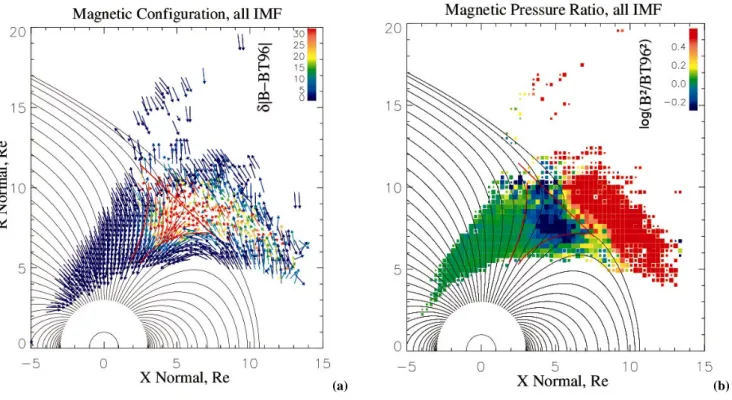
Fig. 3. The statistical spatial distributions of the Cluster FGM magnetic field measurements, for all IMF conditions. (a) The distribution of the magnetic field vectors, which correspond to a projection using the transformations given in Sect. 2. The size of each vector is |B| magnitude in logarithmic scale. The color of the vectors corresponds to the deviation of the measured B and the model B T96 (h|Bmeas−BT96|i). Its magnitude (in nT) is illustrated by the color palette at the top right-hand corner of the figure. (b) The scalar spatial distribution of the ratio between the square of the measured magnetic field (i.e. the pressure) and that from the T96 model in logarithmic scale. The corresponding color scale is presented in the palette at the top right-hand corner of the figure. In both figures, the background field lines presents the T96 “reference” magnetic field. The three boundaries drawn as red curves are simply shown for context and are defined from all the distributions shown in this paper. See text for details.
2.4 Solar wind parameters distributions
Our statistics are based on a large number of orbit points and solar wind conditions (25 427 orbit samples, so the number of solar wind conditions is 5 times smaller). In Fig. 2 we display the distributions of the number of orbit samples as a function of the solar wind dynamic pressure (top left-hand side histogram), Dst index (top right), IMF “clock” angle (CA= tan−1(B
y/Bz)in GSM) (bottom left) and IMF
“gar-den hose” angle (tan−1(B
y/Bx)in GSM) (bottom right).
The distribution of the dynamic pressure is determined from averages over bins of 0.2 nPa. It shows a peak at low pressures, about 1–2 nPa, and it is characterized by a quite sharp tail and the number of samples above 6 nPa is very low (all events above 10 nPa have been removed from the statis-tics). This distribution appears quite typical, as well as that of the Dst index, shown in the top right-hand side histogram of Fig. 2. The latter is basically centered about slightly negative values and shows quite sharp tails. The solar wind dynamic pressure and geomagnetic conditions used in this survey are, on average, relatively quiet.
The clock angle and garden hose angle show more com-plex distributions (the averages are made for bins of 10◦). Two major peaks are observed in both distributions; these
are broadly centered in the intervals 45◦<CA<90◦ and
−135◦<CA<−90◦ for the clock angle. Those peaks are seen near −45◦and 135◦in the case of the garden hose angle. This behavior is well known and attributed to the preferential spiral configuration of the IMF in the ecliptic plane (Parker, 1958). In general, the number of samples is always high, and in the case of southward and northward IMF orientations discussed later, the intervals used have significant statistics.
To investigate the possible effects of the IMF orienta-tion on the cusp flows (Sect. 3.4), we will present distri-butions that arise from the use of restricted IMF clock an-gle ranges, namely, the distributions referred to as south-ward (northsouth-ward) IMF correspond to distributions of orbit points that occurred during conditions of IMF clock angle
|CA|>120◦(<60◦).
3 Results and discussions
In this section, we present and discuss the results of our sta-tistical study. First, in Sect. 3.1 we show the overall magnetic field configuration of the high-altitude cusp, and compare the results with the T96 model field. We then determine the den-sity and temperature distributions in Sect. 3.2. Combined
3014 B. Lavraud et al.: Cluster survey of the high-altitude cusp properties
19
Figure 3. The statistical spatial distributions of the Cluster FGM magnetic field measurements, for all IMF conditions. (Left) The distribution of the magnetic field vectors, which correspond to a projection using the transformations given in section 2. The size of each vector is |B| magnitude in logarithmic scale. The color of the vectors corresponds to the deviation of the measured B and the model B T96 (〈|Bmeas – BT96|〉). Its magnitude (in nT) is illustrated by the color palette at the top right-hand corner of the figure. (Right) The scalar spatial distribution of the ratio between the square of the measured magnetic field (i.e. the pressure) and that from the T96 model in logarithmic scale. The corresponding color scale is presented in the palette at the top right-hand corner of the figure. In both figures, the background field lines presents the T96 “reference” magnetic field. The three boundaries drawn as red curves are simply shown for context and are defined from all the distributions shown in this paper. See text for details.
Figure 4. The spatial distribution of the bulk velocity magnitude from the HIA measurements. In this figure all conditions of IMF are taken into account. The boundary between the exterior cusp and the magnetosheath is clearly distinguished as the strong velocity gradient. A color palette shows the magnitude of the average velocity at the top right-hand corner of the figure.
Fig. 4. The spatial distribution of the bulk velocity magnitude from the HIA measurements. In this figure all conditions of IMF are taken into account. The boundary between the exterior cusp and the magnetosheath is clearly distinguished as the strong velocity gradi-ent. A color palette shows the magnitude of the average velocity at the top right-hand corner of the figure.
with the bulk velocity distribution, it is possible to identify all the boundaries surrounding the low magnetic field exte-rior cusp region. The properties of magnetic, ion and total pressure distributions are analyzed in Sect. 3.3. In Sect. 3.4, we show preliminary results of the bulk plasma flow distribu-tions which illustrate the statistical difference between north-ward and southnorth-ward IMF orientation.
3.1 The exterior cusp diamagnetic cavity
The statistical spatial distribution of the Cluster magnetic field vector measurements is shown in Fig. 3a. The vec-tors are projected into the normalized frame according to the transformations given in Sect. 2. The vectors lengths are pro-portional to the logarithm of the magnetic field magnitudes. The color of the vectors indicates the deviation between the measured magnetic field and the T96 model magnetic field (see caption). This figure makes use of the entire data set for all IMF conditions. By definition, the T96 model field in the magnetosheath is set to the IMF value (Byand Bz
compo-nents, but Bx=0 nT), and does not take into account the actual
compressed nature of the magnetosheath. The T96 model field in the magnetosheath is therefore underestimated and the deviations observed there are not physically meaningful (see the discussion of the external boundary in Sect. 3.2).
However, Fig. 3a clearly suggests that the spatial sampling method is well adapted to the study of the inner magneto-spheric regions. In the left-hand part of the figure in the lobe region, the average magnetic field direction appears to be consistent with that from the background “reference” model field. In addition, the magnitude of the field is also very close to that expected (blue color). A similar agreement is evident in the dayside plasma sheet region; in the cells bounded by 5<XN orm<10 and 5<RN orm<7 (in RE), the magnetic field
orientations and magnitudes are consistent. The boundaries of these two regions appear roughly compatible with the ref-erence model field topology.
In the distant cusp region (R>7 REalong the open-closed
field line separatrix), the measured direction and magnitude gradually depart from the T96 model field with increasing radial distances. This demonstrates the presence of a wide interface between the magnetosheath and the magnetosphere that is not resolved by the T96 model. This region is the low magnetic field exterior cusp.
Figure 3b shows the (scalar) spatial distribution of the ra-tio between the square of the measured magnetic field magni-tude (magnetic pressure) and that from the T96 model. Both the lobes and the dayside plasma sheet show ratios around 1, as expected. However, the exterior cusp region shows a very low magnetic field on average compared to that in the model. This is consistent with the presence of a dense plasma population of magnetosheath origin (see Sect. 3.2).
The T96 model only takes into account a large-scale mag-netopause current (with a symmetric shape approximation) which results in a simple broad vacuum-type low magnetic field region (Tsyganenko, 1995; Tsyganenko and Russell, 1999) near the null points of the cusps (Chapman and Fer-raro, 1931). The combined occurrence of magnetic depres-sion and plasma density enhancement in the transition region observed in our distribution shows the existence of additional diamagnetic current systems; this region is therefore a “dia-magnetic cavity”.
3.2 Characteristics of the boundaries
The distribution of Fig. 3b suggests that the diamagnetic cav-ity is bounded by three distinct boundaries. Two boundaries, respectively, equatorward with the dayside plasma sheet and poleward with the plasma mantle, surround the exterior cusp diamagnetic cavity on its inner edges. The positions of these boundaries were actually defined by the density and temper-ature distributions presented later in this section. It is worth noting that the red curves have been drawn with no particular criteria, and only serve as guides.
A third boundary separates the exterior cusp from the mag-netosheath. The position of this outer boundary is defined by the position of the sharp bulk velocity gradient observed in the velocity distribution shown in Fig. 4 (for all IMF direc-tions). In this figure, the bulk flow appears, on average, to be much lower in the magnetosphere (and the cusp) compared to the adjacent magnetosheath. Further discussion of the flow structure in this region is given in Sect. 3.4.
B. Lavraud et al.: Cluster survey of the high-altitude cusp properties 3015
Figure 5. The density (left) and temperature (right) spatial distributions using the measurements from the HIA instruments. In both cases, all values are shown in logarithmic scale and all IMF orientations are used. The left-hand distribution in fact shows the average of the ratio of the HIA density to the density measured in the solar wind. The right-hand distribution presents the average of the ratio of the HIA temperature to the predicted temperature in the magnetosheath. For this purpose, we make use the actual ACE solar wind measurements and estimate the plasma temperature in the magnetosheath near the cusp by use of the Spreiter et al. (1966) model.
Figure 6. The distributions of the magnetic (B2/2µ
0) (left), ionic (n.kB.T) (middle) and total (right) pressures
normalized to the solar wind ram pressure (ρ.VSW2/2) measured by ACE. The corresponding logarithmic color scale is
shown in the top right-hand corner of each figure. The distributions are made for all solar wind conditions.
(a)
Figure 5. The density (left) and temperature (right) spatial distributions using the measurements from the HIA instruments. In both cases, all values are shown in logarithmic scale and all IMF orientations are used. The left-hand distribution in fact shows the average of the ratio of the HIA density to the density measured in the solar wind. The right-hand distribution presents the average of the ratio of the HIA temperature to the predicted temperature in the magnetosheath. For this purpose, we make use the actual ACE solar wind measurements and estimate the plasma temperature in the magnetosheath near the cusp by use of the Spreiter et al. (1966) model.
Figure 6. The distributions of the magnetic (B2/2µ
0) (left), ionic (n.kB.T) (middle) and total (right) pressures
normalized to the solar wind ram pressure (ρ.VSW2/2) measured by ACE. The corresponding logarithmic color scale is
shown in the top right-hand corner of each figure. The distributions are made for all solar wind conditions.
(b) Fig. 5. The density (a) and temperature (b) spatial distributions using the measurements from the HIA instruments. In both cases, all values are shown in logarithmic scale and all IMF orientations are used. The left-hand distribution, in fact, shows the average of the ratio of the HIA density to the density measured in the solar wind. The right-hand distribution presents the average of the ratio of the HIA temperature to the predicted temperature in the magnetosheath. For this purpose, we make use of the actual ACE solar wind measurements and estimate the plasma temperature in the magnetosheath near the cusp by use of the Spreiter et al. (1966) model.
Figure 5 presents distributions of the density (a) and tem-perature (b) measured by the HIA instruments. In both cases, all IMF orientations are used. The density distribution is shown as the ratio of the measured density to the solar wind density. Similarly, the temperature distribution is shown as the ratio of the measured temperature to that calculated from the solar wind parameters (see figure caption).
The density distribution shows a density ratio larger than unity in the magnetosheath, which is expected (because of the bow shock ahead of the magnetosheath). As expected also, the temperature ratio is seen to be very close to 1 on av-erage in the magnetosheath. Moreover, both the density and temperature ratio distributions are homogeneous in the mag-netosheath, which suggests that the normalization method is successful.
It should be noted that there are a few saturated points (black) in the temperature ratio distribution, which are possi-bly the result of bad measurements that have not been prop-erly removed. However, the temperature distribution shows a consistent behavior globally, in particular when compared to the other distributions already introduced.
The boundaries between the exterior cusp, the dayside plasma sheet and the lobes are seen very clearly in these distributions. The lobes appear cold and tenuous while the dayside plasma sheet is much hotter than any other region. On average, the boundaries between these regions appear gradual, as is to be expected from such a statistical method.
The boundary between the exterior cusp and the magne-tosheath is also visible in these distributions (Fig. 5). Going from the magnetosheath to the exterior cusp, it is character-ized by a decrease in density and an increase in temperature. This property confirms the results obtained in the context of recent case studies by Lavraud et al. (2002) and Cargill et al. (2004).
While the two inner boundaries of the exterior cusp form a funnel (thus an indentation), the external boundary with the magnetosheath shows no clear indentation in the vari-ous distributions presented here. Therefore, it may be con-cluded that the indented magnetopause revealed in the stud-ies of Dunlop et al. (2000) and Eastman et al. (2000) corre-sponds to the inner boundaries of the exterior cusp, identi-fied in the present paper as the high-altitude part of the cusp funnel. On the other hand, Zhou and Russell (1997) found no indentation at the magnetopause. It is therefore proba-ble that the definition these latter authors used corresponds to the external boundary, separating the exterior cusp from the magnetosheath and that also shows no clear indentation in our study. While the inner boundaries may form the “tra-ditional” magnetopause (Paschmann et al., 1976; Haerendel et al., 1978; Russell et al., 2000), the external boundary has recently been proposed as a more suitable magnetopause by Onsager et al. (2001).
3016 B. Lavraud et al.: Cluster survey of the high-altitude cusp properties
20
Figure 5. The density (left) and temperature (right) spatial distributions using the measurements from the HIA
instruments. In both cases, all values are shown in logarithmic scale and all IMF orientations are used. The left-hand
distribution in fact shows the average of the ratio of the HIA density to the density measured in the solar wind. The
right-hand distribution presents the average of the ratio of the HIA temperature to the predicted temperature in the
magnetosheath. For this purpose, we make use the actual ACE solar wind measurements and estimate the plasma
temperature in the magnetosheath near the cusp by use of the Spreiter et al. (1966) model.
Figure 6. The distributions of the magnetic (B
2/2µ
0) (left), ionic (n.k
B.T) (middle) and total (right) pressures
normalized to the solar wind ram pressure (ρ.V
SW2/2) measured by ACE. The corresponding logarithmic color scale is
shown in the top right-hand corner of each figure. The distributions are made for all solar wind conditions.
(a)
20
Figure 5. The density (left) and temperature (right) spatial distributions using the measurements from the HIA
instruments. In both cases, all values are shown in logarithmic scale and all IMF orientations are used. The left-hand
distribution in fact shows the average of the ratio of the HIA density to the density measured in the solar wind. The
right-hand distribution presents the average of the ratio of the HIA temperature to the predicted temperature in the
magnetosheath. For this purpose, we make use the actual ACE solar wind measurements and estimate the plasma
temperature in the magnetosheath near the cusp by use of the Spreiter et al. (1966) model.
Figure 6. The distributions of the magnetic (B
2/2µ
0) (left), ionic (n.k
B.T) (middle) and total (right) pressures
normalized to the solar wind ram pressure (ρ.V
SW2/2) measured by ACE. The corresponding logarithmic color scale is
shown in the top right-hand corner of each figure. The distributions are made for all solar wind conditions.
(b)
20
Figure 5. The density (left) and temperature (right) spatial distributions using the measurements from the HIA
instruments. In both cases, all values are shown in logarithmic scale and all IMF orientations are used. The left-hand
distribution in fact shows the average of the ratio of the HIA density to the density measured in the solar wind. The
right-hand distribution presents the average of the ratio of the HIA temperature to the predicted temperature in the
magnetosheath. For this purpose, we make use the actual ACE solar wind measurements and estimate the plasma
temperature in the magnetosheath near the cusp by use of the Spreiter et al. (1966) model.
Figure 6. The distributions of the magnetic (B
2/2µ
0) (left), ionic (n.k
B.T) (middle) and total (right) pressures
normalized to the solar wind ram pressure (ρ.V
SW2/2) measured by ACE. The corresponding logarithmic color scale is
shown in the top right-hand corner of each figure. The distributions are made for all solar wind conditions.
(c)
Fig. 6. The distributions of the magnetic (B2/2µ0)(a), ionic (n.kB.T) (b) and total (c) pressures normalized to the solar wind ram
pres-sure (ρ.V2SW/2) measured by ACE. The corresponding logarithmic color scale is shown in the top right-hand corner of each figure. The distributions are made for all solar wind conditions.
3.3 Global equilibrium in the exterior cusp region
Figure 6 shows the distributions of the magnetic (B2/2µ0),
ion (n.kB.T) and total pressures normalized to the actual
so-lar wind ram pressure (ρ.V2SW/2). Normalization to the
so-lar wind ram pressure is a rough substitute to normalization to the magnetosheath pressure in the vicinity of the cusp. The thermal pressure of the solar wind is small compared to its ram pressure, and the solar wind kinetic energy is the main source of the magnetosheath pressure. Since the
B. Lavraud et al.: Cluster survey of the high-altitude cusp properties 3017
Figure 7. The distributions of the bulk velocity magnitude for two different IMF orientations; on the left (right) is the distribution for IMF |CA| > 120° (< 60°), thus for a southward (northward) orientation.
(a)
Figure 7. The distributions of the bulk velocity magnitude for two different IMF orientations; on the left (right) is the distribution for IMF |CA| > 120° (< 60°), thus for a southward (northward) orientation.
(b)
Fig. 7. The distributions of the bulk velocity magnitude for two different IMF orientations; (a) and (b) respectively are the distributions for IMF |CA|>120◦(<60◦), thus for a southward and northward orientation respectively.
magnetosheath pressure is a linear function of M2 (M be-ing the solar wind Mach number) (Spreiter et al., 1966), it may be roughly estimated as a linear function of V2SW. The magnetosheath density is roughly proportional to the solar wind density. Hence, for reasonable ranges of M the magne-tosheath pressure is proportional to ρ.V2SW.
The magnetic pressure distribution (Fig. 6a) shows an (in-ner) indentation that is compatible with the locations of the boundaries quoted previously (and also shown here). The ion pressure distribution (Fig. 6b) clearly shows that this low magnetic pressure region corresponds to a high plasma pressure region. The distribution of total pressure (Fig. 6c) does not show any clear indentation within the whole re-gion. There are no latitudinal variations of the total pres-sure and no discontinuities are observed between the exterior cusp and the lobes or the dayside plasma sheet. Yet the ex-ternal boundary with the magnetosheath is also not discern-able. This characteristic demonstrates that the exterior cusp is in equilibrium with its surrounding, at least in a statistical sense.
3.4 IMF orientation dependence of the velocity distribu-tions
In this paper we limit our investigation of the statistical IMF dependence of the cusp structure to the plasma bulk flow magnitude distributions. Future papers will be devoted to more specific, focused studies on this topic.
Figure 7 presents the distributions of the bulk velocity magnitude for two different IMF orientations: Fig. 7a(b) is the distribution for IMF |CA|>120◦(<60◦), thus for a southward (northward) orientation. Although both distribu-tions show, on average, small bulk velocities in the exterior cusp compared to the adjacent magnetosheath (equivalently to Fig. 4), a marked difference is still observed between the two IMF orientations.
Very little flow is measured, on average, in the exterior cusp region for northward IMF. There is, however, little ev-idence for larger flows near the poleward boundary at high-altitudes between 3<XN orm<6 and 8<RN orm<10 (in RE).
However, the sizes of the squares (relative to the amount of samples) in this area render this characteristic questionable. We may point out that such properties would not be incon-sistent with observations from case studies (Fuselier et al., 2000; Lavraud et al., 2002). These were explained in terms of the possible consequences of lobe reconnection, imply-ing plasma precipitation at high-latitudes and a slow sun-ward field line convection (perpendicular flow). Because of the combined presence of a large amount of reflected ions (Lavraud et al., 2003), the exterior cusp region shows both low perpendicular and parallel velocities.
The southward IMF distribution shows a different be-havior. It seems that the flows are, on average, larger for these conditions than for northward IMF, in particular near the plasma sheet boundary at relatively low latitudes (3<XN orm<7 and 6<RN orm<8 RE). These properties
3018 B. Lavraud et al.: Cluster survey of the high-altitude cusp properties reconnection followed by tailward convection of the open
field lines and plasma precipitation at the dayside edge of the cusp (Lockwood and Smith, 1992). A recent Cluster case study by Cargill et al. (2004) showed the presence of very large flows in the exterior cusp under strongly south-ward IMF.
These later results are, however, very preliminary and any possible tendencies will be addressed in the near future through the analysis of the parallel and perpendicular com-ponents of the flows, which should shed some new, important insights in this respect.
4 Summary
We have reported on new statistical results from encounters of the Cluster spacecraft in the high-altitude cusp region dur-ing the first three years of operations. By use of an elabo-rate sampling method we have determined the spatial distri-butions of the ion and magnetic measurements from Cluster which gave an unprecedented opportunity to study the global high-altitude cusp characteristics. The main conclusions that arise from this study may be summarized as follows:
– Although some improvement is still needed, the spa-tial sampling method used here appears well adapted to study this region of the magnetosphere. It allows us to fix the boundaries locations in a proper way.
– The magnetic field vector structure clearly highlights the presence of an intermediate region between the mag-netosheath and the magnetosphere: the exterior cusp. – This region is large and characterized by the presence of
cold dense plasma near the null point of the traditional Chapman-Ferraro (1931) model. Comparison with the Tsyganenko (1995, 1996) magnetic field model demon-strates that this region is diamagnetic in nature. – The density, temperature and velocity distributions have
allowed us to establish the presence of three distinct boundaries surrounding the exterior cusp region: with the lobes, the dayside plasma sheet and the magne-tosheath.
– While the two inner boundaries are well known, the av-erage position of the external boundary with the magne-tosheath has been presented here and is most accurately obtained through the statistical distribution of the bulk velocity. This study further demonstrates that this exter-nal boundary is characterized by a density decrease and a temperature increase, from the magnetosheath to the exterior cusp.
– The two inner boundaries form a funnel which can be viewed as the traditional magnetopause (Paschmann et al., 1976; Haerendel et al., 1978) when observed at high altitude. The external boundary shows no clear indenta-tion in our distribuindenta-tions. In the context of reconnecindenta-tion,
this latter boundary was proposed as a more appropriate magnetopause in a recent paper (Onsager et al., 2001). – The pressure distributions further illustrate that the
ex-terior cusp region is in equilibrium with its surrounding in a statistical sense.
– Finally, preliminary analysis of the bulk flow magnitude distributions suggests that the exterior cusp is overall stagnant under northward IMF conditions (Lavraud et al., 2002), but more convective under southward IMF conditions (Vasyliunas, 1995; Cargill et al., 2004). We finally comment on the ability to analyze averages of the various plasma and field parameters in the exterior cusp region. It has been shown through recent Cluster case studies that this region shows a depressed magnetic field, a slightly lower density and a greater temperature than the adjacent magnetosheath for both southward (Cargill et al., 2004) and northward (Lavraud et al., 2002) IMF orientations. Making averages for the ensemble of the IMF conditions for these parameters is thus meaningful, as further revealed through-out the present paper. It is, however, clearly revealed here that the study of the plasma flows in this region needs the use of restricted IMF clock angle ranges, which will be continued in a forthcoming study.
Acknowledgements. The authors are grateful to the CIS and FGM
teams for their incomparable work in data processing. P. J. Cargill acknowledges support from PPARC through a Senior research Fel-lowship. We thank the ACE MFI and SWEPAM instruments teams and the CDAWeb for providing the ACE data.
Topical Editor T. Pulkkinen thanks two referees for their help in evaluating this paper.
References
Balogh, A., Carr, C. M., Acu˜na, M. H., Dunlop, M. W., Beek, T. J., Brown, P., Fornac¸on, H., Georgescu, E., Glassmeier, K.-H., Harris, J., Musmann, G., Oddy, T., and Schwingenschuh, K.: The Cluster magnetic field investigation: overview of in-flight performance and initial results, Ann. Geophys., 19, No. 10–12, 1207–1217, 2001.
Cargill, P. J., Dunlop, M. W., Lavraud, B., Elphic, R. C., Holland, D. L., Nykyri, K., Balogh, A., Dandouras, I., and R`eme, H.: CLUS-TER encounters with the high altitude cusp: Boundary structure and magnetic field depletions, Ann. Geophys., 22,, No. 5, 1739– 1754, 2004.
Chapman, S. and Ferraro, V. C.: A new theory of magnetic storms, Terr. Magn. Atmosph. Elec., 36, 171–186, 1931.
Dunlop, M. W., Cargill, P. J., Stubbs, T. J., and Wooliams, P.: The high-altitude cusps : HEOS-2, J. Geophys. Res., 105, No. A12, 27 509–27 517, 2000.
Eastman, T. E., Boardsen, S. A., Chen, S.-H., and Fung, S. F.: Con-figuration of high-latitude and high-altitude boundary layers, J. Geophys. Res., 105, No. A10, 23 221–23 238, 2000.
Escoubet, C. P., Smith, M. F., Fung, S. F., Anderson, P. C., Hoffman, R. A., M. Basinska, E., Bosqued, J.-M.: Staircase ion signature in the polar cusp – A case study, Geophys. Res. Lett., 19, No. 17, 1735–1738, 1992.
B. Lavraud et al.: Cluster survey of the high-altitude cusp properties 3019
Fung, S. F., Eastman, T. E., Boardsen, S. A., and Chen, S.-H.: High-altitude Cusp positions sampled by the Hawkeye satellite, Phys. Chem Earth, 22, 653–662, 1997.
Fuselier, S. A., Trattner, K. J., and Petrinec, S. M.: Cusp observa-tions of high and low-laltitude reconnection for northward IMF, J. Geophys. Res., 105, No. A1, 253–266, 2000.
Grigoriev, A., Fedorov, A., Budnik, E., et al.: Magnetospheric Mag-netic Field in the Outer Cusp Region: Comparison of Measure-ments Obtained from the INTERBALL-1 Satellite and from the T96 Model, Cosmic Res. (English translation of Kosmicheskie Issledovaniya), Vol. 37, 594, 1999.
Haerendel, G., Paschmann, G., Sckopke, N., Rosenbauer, H., and Hedgecock, P. C.: The Frontside Boundary Layer of the Magne-tosphere and the Problem of Reconnection, J. Geophys. Res., 83, No. A7, 3195–3216, 1978.
Lavraud, B., Dunlop, M. W., Phan, T. D., R`eme, H., Bosqued, J. M., Dandouras, I., Sauvaud, J.-A., Lundin, R., Taylor, M. G. G. T., Cargill, P. J., Mazelle, C., Escoubet, C. P., Carlson, C. W., McFadden, J. P., Parks, G. K., Moebius, E., Kistler, L. M., Bavassano-Cattaneo, M.-B., Korth, A., Klecker, B. and Balogh, A.: Cluster observations of the exterior cusp and its surrounding boundaries under northward IMF, Geophys. Res. Lett., 29, No. 20, 56–60, doi:10.1029/2002GL015464, 2002.
Lavraud, B., R`eme, H., Dunlop, M. W., Bosqued, J. M., Dandouras, I., Sauvaud,J.-A., Keiling, A., Phan, T. D., Lundin, R., Cargill, P. J., Escoubet, C. P., Carlson, C. W., McFadden, J. P., Parks, G. K., Moebius, E., Kistler, L. M., Amata, E., Bavassano-Cattaneo, M.-B., Korth, A., Klecker, B., and Balogh, A.: Cluster observes the high-altitude cusp region, Surv. Geophys., in press, 2004. Lockwood, M. and Smith, M. F.: The variation of reconnection rate
at the dayside magnetopause and cusp ion precipitation, J. Geo-phys. Res., 97, No. A10, 14 841–14 847, 1992.
M˘erka, J., ˇSafr´ankov´a, J., and N˘eme˘cek, Z.: Cusp-like plasma in high altitudes: A statistical study of the width and location of the cusp from Magion-4, Ann. Geophys., 20, No. 3, 311–320, 2002. Newell, P. T. and Meng, C. I.: The cusp and the cleft/LLBL: Low altitude identification and statistical local time variation, J. Geo-phys. Res, 93, No. A12, 14 549–14 556, 1988.
Newell, P. T., Meng, C. I., Sibeck, D. G., and Lepping, P.: Some low-altitude cusp dependencies on the interplanetary magnetic field, J. Geophys. Res, 94, No. A7, 8921–8927, 1989.
Newell, P. T. and Meng, C. I.: Ionospheric projections of magne-tospheric regions under low and high solar wind pressure condi-tions, J. Geophys. Res., 99, 273–286, 1994.
Onsager, T. G., Scudder, J. D., Lockwood, M. and Russell, C. T.: Reconnection at the high latitude magnetopause during north-ward interplanetary magnetic field conditions, J. Geophys. Res., 106, , No. A11, 25 467–24 488, 2001.
Parker, E. N.: Dynamics of interplanetary gas and magnetic fields, Astrophys. J., 128, 664–676, 1958.
Paschmann, G., Haerendel, G., Sckopke, N., Rosenbauer, H. and Hedgecock,P. C.: Plasma and Magnetic Field Characteristics of the Distant Polar Cusp Near Local Noon: The Entry Layer, J. Geophys. Res., 81, No. 16, 2883–2899, 1976.
R`eme, H., Aoustin, C., Bosqued, J. M., Dandouras, I., Lavraud, B., Sauvaud, J.-A., Barthe, A., Bouyssou, J., Camus, T., Cœur-Joly, O., Cros, A., Cuvilo, J., Ducay, F., Garbarowitz, Y., M´edale, J. L., Penou, E., Perrier, H., Romefort, D., Rouzaud, J., Vallat, C., Alcayd´e, D., Jacquey, C., Mazelle, C., d’Uston, C., et al.: First multispacecraft ion measurements in and near the earth’s mag-netosphere with the identical CLUSTER Ion Spectrometry (CIS) Experiment, Ann. Geophys., 19, No. 10–12, 1303–1354, 2001. Russell, C. T., Le, G., and Petrinec, S. M.: Cusp observations of
high and low latitude reconnection under northward IMF: and alternate view, J. Geophys. Res., 105, No. A3, 5489–5495, 2000. Shue, J.-H., Chao, J. K., Fu, H. C., Russell, C. T., Song, P., Khurana, K. K., Singer, H. J.: A new functional form to study the solar wind control of the magnetopause size and shape, J. Geophys. Res., 102, No. A5, 9497–9511, 1997.
Spreiter, J. R., Alksne, A. Y., and Abraham-Shrauner, B.: Theoreti-cal proton velocity distributions in the flow around the magneto-sphere, Planet. Space Sci., 14, No. 11, 1207–1220, 1966. Spreiter, J. R. and Summers, A. L.: On the conditions near the
neu-tral points on the magnetosphere boundary, Planet. Space Sci., 15, No. 4, 787–798, 1967.
Tsyganenko, N. A.: A magnetospheric magnetic field model with a warped tail current sheet, Planet. Space Sci., 37, No. 1, 5–20, 1989.
Tsyganenko, N. A.: Modeling the Earth’s magnetospheric magnetic field confined within a realistic magnetopause,J. Geophys. Res., 100, No. A4, 5599–5612, 1995.
Tsyganenko, N. A.: Effects of the solar wind conditions on the global magnetospheric configuration as deduced from data-based field models, Eur. Space Agency Spec. Pub., ESA SP-389, 181, 1996.
Tsyganenko, N. A. and Russell, C. T.: Magnetic signatures of the distant polar cusps: Observations from Polar and quantitative modeling, J. Geophys. Res., 104,No. A11, 24 939–24 955, 1999. Vasyliunas, V. M.: Multi-branch model of the open magnetopause,
Geophys. Res. Lett., 22, No. 9, 1245–1247, 1995.
Woch, J. and Lundin, R.: Magnetosheath plasma precipitation in the polar cusp and its control by the interplanetary magnetic field, J. Geophys. Res., 97, No. A2, 1421–1430, 1992.
Yamauchi, M., Nilsson, H., Eliasson, L., Norberg, O., Boehm, M., Clemmons, J. H., Lepping, R. P., Blomberg, L., Ohtani, S.-I., Ya-mamoto, T., Mukai, T., Terasawa, T., and Kokubun, S.: Dynamic response of the cusp morphology to the solar wind: A case study during passage of the solar wind plasma cloud on February 21, 1994, J. Geophys. Res., 101, No. A11, 24 675–24 687, 1996. Zhou, X.-W and Russell, C. T.: The location of the high-latitude
polar cusp and the shape of the surrounding magnetopause, J. Geophys. Res., 102, No. A1, 105–110, 1997.
Zhou, X.-W., Russell, C. T., Le, G., and. Fuselier, S. A: The polar cusp location and its dependence on dipole tilt, Geophys. Res. Lett., 26, No. 3, 429–432, 1999.
Zhou, X.-W., Russell, C. T., Le, G., Fuselier, S. A., and Scudder, J. D.: Solar wind control of the polar cusp at high altitude, J. Geophys. Res., 105, No. A1, 245–251, 2000.