Enlarged Krylov Subspace Methods and Preconditioners for Avoiding Communication

(1)

HAL Id: tel-01165960

https://tel.archives-ouvertes.fr/tel-01165960

Submitted on 21 Jun 2015

HAL is a multi-disciplinary open access

archive for the deposit and dissemination of sci-entific research documents, whether they are pub-lished or not. The documents may come from teaching and research institutions in France or abroad, or from public or private research centers.

L’archive ouverte pluridisciplinaire HAL, est destinée au dépôt et à la diffusion de documents scientifiques de niveau recherche, publiés ou non, émanant des établissements d’enseignement et de recherche français ou étrangers, des laboratoires publics ou privés.

for Avoiding Communication

Sophie Moufawad

To cite this version:

Sophie Moufawad. Enlarged Krylov Subspace Methods and Preconditioners for Avoiding Communi-cation. General Mathematics [math.GM]. Université Pierre et Marie Curie - Paris VI, 2014. English. �NNT : 2014PA066438�. �tel-01165960�

(2)

Universit´e Pierre et Marie Curie

´Ecole Doctorale de Sciences Math´ematiques de Paris Centre 386 Laboratoire Jacques-Louis Lions / Equipe Alpines

T

H

ESE DE DOCTORAT

`

Discipline : Math´ematiques Appliqu´ees

pr´esent´ee par

Sophie M

OUFAWAD

Enlarged Krylov Subspace Methods and

Preconditioners for Avoiding Communication

dirig´ee par Laura G

RIGORI

Soutenue le ** 2014 devant un jury compos´e de :

M. Pr´enom N

OM

Universit´e pr´esident

M

lle

_{Pr´enom N}

_OM

_Institut

_examinateur

M

me

_{Pr´enom N}

_OM

_{Universit´e rapporteur}

M. Pr´enom N

OM

Universit´e directeur

(3)

Boite courrier 187 4, place Jussieu 75252 Paris cedex 05 Boite courrier 188 4, place Jussieu 75252 Paris cedex 05

(4)

Chapter 1 Introduction

Many scientific problems require the solution of systems of linear equations of the form Ax “ b, where A is an n ˆ n matrix and b is an n ˆ 1 vector. There are two broad categories for solving systems of linear equations, direct methods and iterative methods. Direct methods solve the system in a finite number of steps or operations. Examples of direct methods are matrix decompositions like LU decomposition A “ LU, Cholesky decomposition for symmetric positive definite A “ LLt_{, and QR decomposition for full rank A “ QR, where L is a lower triangular matrix, U and R}

are upper triangular matrices, and Q is an orthonormal matrix. After decomposing the matrix A, the upper triangular and lower triangular systems are solved by backward and forward substitution. The matrix A can be a dense or a sparse matrix. Several libraries that implement direct methods for solving sparse systems have been introduced, like MUMPS [1], PARADISO [69, 55], and SuperLU [57, 58]. However, when the matrix A is sparse, the factors obtained after decomposition are denser than the input matrix. Moreover, direct methods are prohibitive in terms of memory and flops when it comes to solving very large systems, and they are not easily parallelized on modern-day architectures. Thus, iterative methods that compute a sequence of approximate solutions for the system Ax “ b by starting from an initial guess, are a good alternative.

We are interested in solving systems of linear equations, Ax “ b, where the matrix A is sparse. Such systems may arise from the dicretization of partial differential equations. The Krylov sub-space methods are among the most practical and popular iterative methods today. They are polyno-mial iterative methods that aim to solve systems of linear equations (Ax “ b) by finding a sequence of vectors x1, x2, x3, x4, ..., xkthat minimizes some measure of error over the corresponding spaces

x0` KipA, r0q, i “ 1, ..., k

where x0is the initial iterate, r0is the initial residual, and KipA, r0q “ spantr0, Ar0, A2r0, ..., Ai´1r0u

is the Krylov subspace of dimension i. Conjugate Gradient (CG) [47], Generalized Minimal Resid-ual (GMRES) [66], bi-Conjugate Gradient [56, 30] and bi-Conjugate Gradient Stabilized [75] are some of the Krylov subspace methods. These methods compute one basis vector or one search direction vector at each iteration i, by performing a matrix-vector multiplication. Then, the ith

(9)

approximate solution is defined by performing saxpy (ax ` y) and dot products (xt_{x), where a is}

scalar, and x, y are vectors.

The performance of an algorithm on any architecture is dependent on the processing unit’s speed for performing floating point operations (flops) and the speed of accessing memory and disk. Moreover, the efficiency of parallel implementations is dependent on the amount of per-formed computations per communication, data movement. This is due to the fact that the cost of communication is much higher than arithmetic operations, and this gap is expected to continue to increase exponentially [37]. As a result, communication is often the bottleneck in numerical algorithms. In a quest to address the communication problem, recent research has focused on re-formulating linear algebra operations such that the movement of data is significantly reduced, or even minimized as in the case of dense matrix factorizations like LU factorization, QR factoriza-tion, tall and skinny QR factorization [21, 38, 4]. Such algorithms are referred to as communication avoiding.

The Krylov subspace methods are governed by Blas1 and Blas2 operations like dot products and matrix vector multiplications, as discussed above. Parallelizing dot products is constrained by communication, since the performed computation is negligible. If the dot products are performed by one processor, then there is a need for a communication before (synchronization) and after the computations. In both cases, communication is a bottleneck. This problem has been tackled by different approaches. One approach is to the hide the communication’s cost by overlapping it with other communications and computations, like pipelined CG [23, 43] and pipelined GMRES [34]. Another approach consists of replacing Blas1 and Blas2 operations by Blas2 and Blas3 operations, by either introducing new methods or by reformulating the algorithm itself. The first such methods to be introduced, are block methods that solve a system with multiple right-hand sides AX “ B, like O’Leary’s block CG [63]. These methods compute at each iteration a block of vectors by performing a matrix times a block of vectors. Then, the ith_{block approximate solution is obtained}

by solving small systems and performing tall skinny gaxpy’s, Ax ` y, where A is an n ˆ m matrix with n °° m, and x, y are vectors.

Unlike the block methods, the s-step methods solve the system Ax “ b by computing s basis vectors per iteration and solving small systems. Some of the s-step methods are s-step CG [19] and s-step GMRES [26]. Both methods, block and s-step, use Blas2 and Blas3 operations. Recently, communication avoiding Krylov methods, based on s-step methods, were introduced, like CA-CG, and CA-GMRES [60, 48, 12]. The communication avoiding methods aim at further avoiding communication in the Blas2 and Blas3 at the expense of performing some redundant flops. For s _{“ 1, where s-step methods are equivalent to classical methods, there are many available} pre-conditioners. One of them, block Jacobi, is a naturally parallelizable and communication avoiding preconditioner. However, except a discussion in [48], there are no available preconditioners that avoid communication and can be used with s-step methods for s ° 1. This is a serious limitation of these methods, since for difficult problems, Krylov subspace methods without preconditioner can be very slow or even might not converge. In this thesis, we introduce a communication avoiding ILU(0) preconditioner (CA-ILU0) [40], that can be computed in parallel, and applied to s vectors

(10)

CHAPTER 1. INTRODUCTION 7 of the form yi “ pLUq´1Ayi´1without any communication, for i “ 1, 2, .., s. This preconditioner

can be parallelized without communication due to the use of a heuristic reordering of the matrix A, that we call alternating min-max layersAMML(s). Moreover, the CA-ILU0 preconditioner can

also be used with classical Krylov subspace methods, where it avoids communication.

Since communication avoiding methods are based on s-step methods which have some stabil-ity issues, we introduce a new type of Krylov subspace methods. We introduce a new approach that consists of enlarging the Krylov subspace based on domain decomposition. First, we split the initial r0 into t vectors depending on a decomposed domain. Then, the obtained t vectors

are multiplied by A at each iteration to generate the t new basis vectors of the enlarged Krylov subspace. Enlarging the Krylov subspace should lead to faster convergence and parallelizable al-gorithms with less communication than the classical Krylov methods, due to the use of Blas2 and Blas3 operations. In this thesis, we introduce two new versions of conjugate gradient. The first version, multiple search direction with orthogonalization CG (MSDO-CG), has the same structure as the classical conjugate gradient method, where we first define t new search directions, then find the t step lengths by solving a tˆt system and update the solution and the residual. But unlike CG, the search directions are not A-orthogonal. We A-orthonormalize the search directions, to obtain a projection method that guarantees convergence at least as fast as CG. The second version, long recurrence enlarged CG (LRE-CG), is similar to GMRES in that we build an orthonormal basis for the enlarged Krylov subspace rather than finding search directions. Then, we use the whole basis to update the solution and the residual.

The thesis is organized as follows. In chapter 2 we briefly introduce some notations and ker-nels that are used throughout this thesis such as graphs and graph partitioning, orthonormalization schemes, A-orthonormalization schemes, the matrix powers kernel, and the set of test matrices used to test our introduced methods. In chapter 3 we discuss several variants of Krylov subspace methods, such as classical Krylov subspace methods (CG and GMRES), block Krylov methods (block CG), s-step Krylov methods (s-step CG and s-step GMRES), communication avoiding Krylov methods (CA-GMRES), and other parallelizable version (MSD-CG and coop-CG). We also discuss preconditioners, such as incomplete LU preconditioner, block Jacobi preconditioner, and restricted additive Schwarz preconditioner, which are crucial for the fast convergence of Krylov subspace methods.

In chapter 4 we introduce the enlarged Krylov subspace, the MSDO-CG method, and the LRE-CG method. We show that both methods are projection methods and hence converge at least as fast as CG in exact precision. And we compare the convergence behavior of MSDO-CG and LRE-CG methods using different A-orthonormalization and orthonormalization methods. Then we compare the most stable versions with CG and other related methods. Both methods converge faster than CG, but LRE-CG converges faster than MSDO-CG since it uses the whole basis to update the solution rather than only t search directions. We also present the parallel algorithms with their expected performance, and the preconditioned versions with their convergence behavior. This chapter is based on the article [41] which is in preparation for submission.

(11)

minimizes communication during the construction of M “ LU (i.e, the ILU(0) factorization), and during its application to s vectors (z “ M´1_y_{“ pLUq}´1_y_{q) at each iteration of the s-step methods.}

In other words, it is possible to solve s upper triangular system and s lower triangular system, in addition to the s matrix vector multiplications without any communication. First, we adapt the matrix powers kernel to the case of ILU preconditioned systems. Then, we introduce theAMML(s)

heuristic reordering based on nested dissection and k-way graph partitioning. Then, we show that our reordering does not affect the convergence of ILU(0) preconditioned GMRES, and we model the expected performance of our preconditioner based on the needed memory and the redundant flops introduced to reduce the communication. This chapter is based on some parts of a revised version of the technical report [40], and on the article [39], which was submitted to SIAM journal on scientific computing (SISC) and is in revision. Finally, in chapter 6 we conclude and discuss possible future work in the introduced methods.

(12)

Chapter 2 Preliminaries

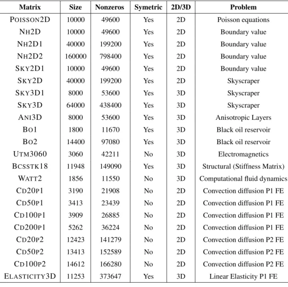
We will briefly introduce some notations (section 2.1) and kernels that will be used throughout this thesis such as graphs and graph partitioning (section 2.2), orthonormalization (section 2.3), A-orthonormalization (section 2.4), and the matrix powers kernel (section 2.5) . We will also describe the test matrices (section 2.6) that will be used in Chapters 4 and 5.

2.1 Notation

We denote matrices or block of vectors by upper case letters. Whereas vectors are denoted by lower case letters. All subscripts used for matrices, vectors, graphs, and sets serve as indices, indices denoting iterations (xk) or subparts (A1,1). We use matlab notation for matrices and vectors. For

example, given a vector y of size n ˆ 1 and a set of indices ↵ (which correspond to vertices in the graph of A), yp↵q is the vector formed by the subset of the entries of y whose indices belong to ↵. For a matrix A, Ap↵, :q is a submatrix formed by the subset of the rows of A whose indices belong to ↵. Similarly, Ap:, ↵q, is a submatrix formed by the subset of the columns of A whose indices belong to ↵. We have Ap↵, q “ rAp↵, :qsp:, q, the columns of the submatrix Ap↵, :q. Note that the set of indices can be expressed explicitly like yp1 : 20q which is a vector with the first 20 entries of y or Ap:, 1 : tk ` i ´ 1q which is a matrix containing the first tk ` i ´ 1 columns of A.

2.1.1 Communication

In this thesis, the word “processor” indicates the component performing the computations and “fetch” indicates the data movement. The definition of this “processor” and “fetch” depends on the kind of communication that we want to avoid. The two broad categories are communication in parallel computations (between processors) and communication in sequential computations (be-tween different levels of memory hierarchy)

In the first case, communication can take the following forms, among others: 9

(13)

• Messages between processors, in a distributed-memory system. (“processor” = processor, “fetch” = receive message)

• Cache coherency traffic, in a shared-memory system. (“processor” = core, “fetch” = read) • Data transfers between coprocessors linked by a bus, such as between a CPU (“Central

Processing Unit” or processor) and a GPU (“Graphics Processing Unit”). (“processor” = GPU, “fetch” = copy from CPU memory to GPU memory)

In the sequential case, communication between levels of hierarchy can be between: • cache and main memory.

• main memory and disk.

• local store (a small, fast, software-managed memory ) and main memory.

In the three cases of sequential communication, the “processor” = processor and by “fetch” we mean copy the data from the slow memory to the fast one.

In general, the estimated time for computing z flops is cz, where c is the inverse

floating-point rate, also called the floating-floating-point throughput (seconds per floating-floating-point operation) of the processor. In the case of distributed-memory architecture, the estimated time for sending a mes-sages of size k is ↵c ` ck, where ↵c is the latency (with units of seconds) and c is the inverse

bandwidth (seconds per word). Hence, the estimated runtime of an algorithm with a total of z computed flops and s sent messages each of size k is the sum of their corresponding estimated times cz` ↵cs` c.

2.2 Graphs and partitioning techniques

In this section we give the definitions of the notions such as graphs (section 2.2.1), nested dissection (section 2.2.2), and k-way partitioning (section 2.2.3).

2.2.1 Graphs

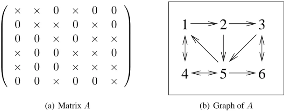
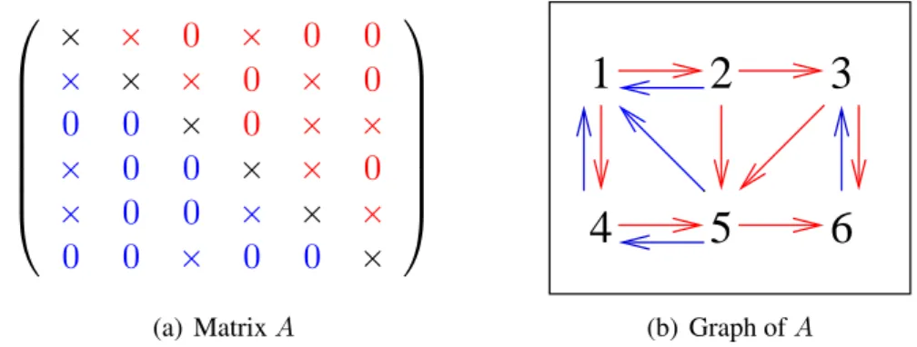
The structure of an unsymmetric n ˆ n matrix A can be represented by using a directed graph G_{pAq “ pV, Eq, where V is a set of vertices and E is a set of edges. A vertex v}iis associated with

each row i of the matrix A. An oriented edge ej,ifrom vertex j to vertex i is associated with each

nonzero element Apj, iq “ 0 as shown in Figure 2.1 where the vertex is represented by its index. A weight wi and a cost cj,i are assigned to every vertex vi and edge ej,i respectively. Let B be a

subgraph of GpAq (B Ä GpAq), then V pBq is the set of vertices of B, V pBq Ä V pGpAqq, and EpBq is the set of edges of B, EpBq Ä EpGpAqq. Let i and j be two vertices of GpAq. The vertex

(14)

CHAPTER 2. PRELIMINARIES 11

¨

˚

˝

ˆ ˆ 0 ˆ 0 0

0 ˆ ˆ 0 ˆ 0

0

0 ˆ 0 ˆ ˆ

ˆ 0 0 ˆ ˆ 0

ˆ 0 0 ˆ ˆ ˆ

0

0 ˆ 0 0 ˆ

˛

‹

‚

1

(a) Matrix A

2

4

5

6

1

3

(b) Graph of A

Figure 2.1: The figure shows the sparsity pattern of a matrix A and its corresponding graph.

j is reachable from the vertex i if and only if there exists a path of directed edges from i to j. The length of the path is equal to the number of visited vertices excluding i. Let S be any subset of vertices of GpAq. The set RpGpAq, Sq denotes the set of vertices reachable from any vertex in S and includes S (S Ä RpGpAq, Sq). The set RpGpAq, S, mq denotes the set of vertices reachable by paths of length at most m from any vertex in S. The set RpGpAq, S, 1q is the set of adjacent vertices of S in the graph of A and we denote it by AdjpGpAq, Sq. The set AdjpGpAq, Sq ´ S is the open set of adjacent vertices of S in the graph of A and we denote it by opAdjpGpAq, Sq. An undirected graph of a symmetric matrix is a special case of directed graphs where all the edges are bidirectional. Since there is no need to specify a direction, the edges are undirected.

Note that the structure of a sparse matrix can also be represented by a hypergraph H “ pV, N q, where V is a set of vertices and N is a set of hyperedges (nets) where each hyperedge can connect several vertices.

To exploit parallelism and reduce communication when solving a linear system Ax “ b using an iterative solver, the input matrix A is often reordered using graph partitioning techniques such as nested dissection [33, 52] or k-way graph partitioning [51]. These techniques assume that the matrix A is symmetric and its graph is undirected. In case A is unsymmetric, then the undirected graph of A ` At _{is used to define a partition for the matrix A. Graph partitioning techniques can}

be applied on both graphs and hypergraphs (see e.g. [13, 3]), and they rely on identifying either edge/hyperedge separators or vertex separators. In sections 2.2.2 and 2.2.3 we describe Nested Dissection and K-way briefly in the context of undirected graphs.

2.2.2 Nested dissection

Nested dissection [33] is a divide and conquer graph partitioning strategy based on vertex sepa-rators. For undirected graphs, at each step of dissection, a set of vertices that forms a separator is sought, that splits the graph into two disjoint subgraphs once the vertices of the separator are removed. We refer to the two subgraphs as ⌦1,1and ⌦1,2, and to the separator as ⌃1,1. The vertices

(15)

of the first subgraph are numbered first, then those of the second subgraph, and finally those of the separator. The corresponding matrix has the following structure,

A“ ¨ ˝ A11 A22 AA1323 A31 A32 A33 ˛ ‚.

The algorithm then continues recursively on the two subgraphs ⌦1,1 and ⌦1,2. The separators

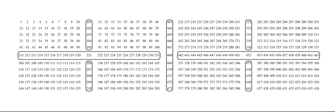
subgraphs and the subdomains subgraphs introduced at level i of the nested dissection are denoted by ⌃i,j and ⌦i,l respectively, where j § 2i´1, l § 2i, i § t and t “ logpP q (P is the number of

processors). The vertices of the separators and the final subdomains are denoted by Si,j “ V p⌃i,jq

and Dl “ V p⌦t,lq respectively. Thus, at level i we introduce 2i´1 new separators and 2i new

subdomains. We illustrate nested dissection in Figure 2.2 which displays the graph of a 2D 5 point-stencil matrix A, where the vertices are represented by their indices. For clarity of the figure, the edges are not shown in the graph, but it must be noted that there are oriented edges connecting each vertex to its north, south, east and west neighbors. This corresponds to a symmetric matrix with a maximum of 5 nonzeros per row. Figure 2.2 presents the subdomains and the separators obtained by using three levels of nested dissection. All the following figures of graphs in this thesis have the same format.

221 463 464 465 467 466 473 470 471 472 469 468 233 234 235 245 244 243 253 254 255 256 246 236 247 257258259260 248 249 250 239 238 237 240 273 274 275 276 277 278 279 280 263 264 265 266 267 268 269 270 378 379 380 381 382 383 384 385 350 349 348 368 358 359 369 370 360 371 361 351 352 362 372 373 374 375 365 364 363 353 354 355 282 283 284 285 295 294 293 292 302 303 304 305 306 296 286 297 307308309310311 298 299 300 301 291 289 288 287 290 322 323 324 325 326 327 328 329 330 331 312 313 314 315 316 317 318 319 320 321 427 428 429 430 431 432 433 434 435 436 388 389 390 400 399 398 397 407 417 418 408 409 419 420 410 421 411 401 391 402 412 422 423 424 425 426 416 415 414 413 403 404 405 406 396 394 393 392 395 387 338 339 340 341342343344345 443 444 445 446447448449450 453454 455 456 457458459460461462 261 251 241 281 271 386 376 366 356 346 451 334 333 332 336 335 441 440 439 438 437 452 232 242 252 272 262 377 347 357 367 337 442 1 2 3 4 14 13 12 11 21 22 23 24 25 15 5 16 26272829 17 18 19 8 7 6 9 41 42 43 44 45 46 47 48 49 31 32 33 34 35 36 37 38 39 146 147 148 149 150 151 152 153 154 119 118 117 116 126 136 137 127 128 138 139 129 140 130 120 121 131 141 142 143 144 134 133 132 122 123 124 51 52 53 54 64 63 62 61 71 72 73 74 75 65 55 66 7677787980 67 68 69 70 60 58 57 56 59 91 92 93 94 95 96 97 98 99 100 81 82 83 84 85 86 87 88 89 90 196 197 198 199 200 201 202 203 204 205 157 158 159 169 168 167 166 176 186 187 177 178 188 189 179 190 180 170 160 171 181 191 192 193 194 195 185 184 183 182 172 173 174 175 165 163 162 161 164 156 107 108 109 110111112113114 106 212 213 214 215216217218219 211 222223 224 225 226227228229230231 30 20 10 50 40 155 145 135 125 115 220 103 102 101 105 104 210 209 208 207 206

Figure 2.2: An 11 by 43 5-point stencil, partitioned into 8 subdomains using 7 separators . The bidirectional edges connecting each vertex to its north, south, east and west neighboring vertices are omitted in this figure.

2.2.3 K-way graph partitioning

K-way graph partitioning by edge separators aims at partitioning a graph G “ pV, Eq into k ° 1 parts ⇡ “ t⌦1, ⌦2, .., ⌦k´1, ⌦ku, where the k parts are nonempty (⌦i ‰ , ⌦i Ä V for 1 § i § k,

and Yk

i“1⌦i “ V ), and the partition ⇡ respects the balance criterion

(16)

CHAPTER 2. PRELIMINARIES 13 where Wi “∞_vjP⌦iwjis the weight associated to each part ⌦i, Wavg “ p∞_viPV wiq{k is the perfect

weight, ✏ is the maximum allowed imbalance ratio, and wjis the weight associated to vertex vj. In

addition, k-way graph partitioning minimizes the cutsize of the partition ⇡ p⇡q “ ÿ

ei,jPEE

ci,j, (2.2)

where EE is the set of external edges of ⇡, EE Ä E, and ci,j is the cost of the edge ei,j where i † j.

In graph partitioning, the term edge-cut indicates that the two vertices that are connected by an edge belong to two different partitions. The edge which is cut is referred to as an external edge. In this thesis, we use wj “ 1 and ci,j “ 1.

2.3 Orthonormalization

Given an n ˆ tk matrix Q whose tk column vectors are orthonormal and an n ˆ t matrix Pk`1, we

discuss in this section how to obtain tpk ` 1q orthonormal vectors. This will be used in chapters 3 and 4 for describing CA-GMRES and LRE-CG where at each iteration k, t new vectors are com-puted and have to be orthonormalized against the previously comcom-puted tk orthonormal vectors. Let D “ rQ, Pk`1s, then this can be done by orthonormalizing Dp:, tk ` iq against all the previous

vectors of D, Dp:, 1 : ptk ` i ´ 1qq, for 1 § i § t using classical Gram Schmidt or modified Gram Schmidt. However, this can not be parallelized efficiently. Thus, it is better to split the orthonor-malization into two tasks. The first consists of orthonormalizing the t newly computed vectors of Pk`1 against all the tk orthonormal vectors of Q. Then, the vectors of Pk`1 are orthonormalized

against each others.

Orthonormalizing a tall and skinny nˆt matrix Pk`1, can be done using classical Gram Schmidt

(CGS), modified Gram Schmidt (MGS) or a QR factorization like Householder factorization or based on Cholesky factorization. In [21], the authors presented a parallelizable QR version of a tall and skinny matrix based on binary reduction trees with local householder QR which they called tall and skinny QR (TSQR) factorization. As for the orthonormalization of Pk`1against Q, this can

be done using MGS or CGS and its block version. We will briefly discuss CGS orthonormalization (section 2.3.1), MGS orthonormalization (section 2.3.2), and TSQR (section 2.3.3).

2.3.1 Classical Gram Schmidt (CGS)

We will start by introducing the orthonormalization of Pk`1’s vectors against Q’s vectors, then

against each others using CGS.

Assuming that the vectors of Qkare orthonormal , i.e. QtkQk “ I for all j “ 1, 2, .., tk, then

the orthonormalization of the vectors of Pk`1 against the vectors of Qk is defined by projecting

(17)

1, 2, ..., t, by letting rP_k`1_{p:, jq “ P}_k`1_{p:, jq ´}∞tk_i_“1_pQkp:, iqtPk`1p:, jqqQkp:, iq, we get

r

Pk`1p:, jqtQkp:, oq “ Pk`1p:, jqtQkp:, oq ´∞tki“1pQkp:, iqtPk`1p:, jqqQkp:, iqtQkp:, oq

“ Pk`1p:, jqtQkp:, oq ´ pQkp:, oqtPk`1p:, jqqQkp:, oqtQkp:, oq

“ 0 for all o “ 1, 2, ..., tk since Qt

kQk“ I.

Algorithm 1 Orthonormalization against previous vectors with CGS

Input: Qk, the tk orthonormal vectors; Pk`1, the t vectors to be orthonormalized against Q

Output: rPk`1, the vectors orthonomalized against Q 1: Let rPk`1 “ Pk`1 2: for j “ 1 : t do 3: for i “ 1 : tk do 4: Prk`1p:, jq “ rPk`1p:, jq ´ pQkp:, iqtPk`1p:, jqqQkp:, iq 5: end for 6: Prk`1p:, jq “ _{|| r}_Pk`1p:,jq||2Pk`1p:,jqr 7: end for

Algorithm 2 Orthonormalization against previous vectors with BCGS

Input: Qk, the tk orthonormal vectors; Pk`1, the t vectors to be orthonormalized against Q

Output: rPk`1, the vectors orthonomalized against Q

1: Pr_k`1 _{“ P}_k`1_{´ Q}kpQtkPk`1q

2: for j “ 1 : t do

3: Prk`1p:, jq “ _{|| r}_PPkr_k`1p:,jq||2`1p:,jq 4: end for

Algorithm 3 Orthonormalization of tall and skinny matrix using CGS Input: Pk`1, the matrix to be orthonormalized

Output: Pk`1, the orthonomalized matrix (Pkt`1Pk`1 “ I) 1: Let rPk`1 “ Pk`1 2: for i “ 1 : t do 3: for j “ 1 : pi ´ 1q do 4: Pr_k`1_{p:, iq “ r}P_k`1_{p:, iq ´ p r}P_k`1_{p:, jq}t_P k`1p:, iqq rPk`1p:, jq 5: end for 6: Prk`1p:, iq “ _{|| r}_PPr_k`1p:,iq||2k`1p:,iq 7: end for

(18)

CHAPTER 2. PRELIMINARIES 15 Algorithm 1 summarizes the CGS orthonormalization of Pk`1’s vectors against Qk. However,

a better parallelizable block version of the algorithm can be presented by eliminating the for loops as shown in Algorithm 2. As for the orthonormalization of the tall and skinny matrix Pk`1 using

CGS, it follows the same pattern as shown in Algorithm 3. In [71], the authors present a more stable version of CGS (Algorithm 3) that differs in the normalization step. The normalization in Algorithms?? could be changed accordingly.

2.3.2 Modified Gram Schmidt (MGS)

It is known that CGS has some numerical stability problems due to the errors resulting from the projection of the initial vector repeatedly against all other vectors [36, 71] , i.e. rPk`1p:, jq “ Pk`1p:

, jq ´∞tk_i“1pQkp:, iqtPk`1p:, jqqQkp:, iq. The modified Gram Schmidt partially fixes this issue by

orthogonalizing the initial vector Pk`1p:, jq against Qkp:, 1q and then the obtained vector rPk`1p:, jq

is orthogonalized against Qkp:, 2q and so on. We will start by introducing the orthonormalization of

Pk`1’s vectors against Qk’s vectors, then against each others using MGS. Algorithm 4 summarizes

the MGS orthonormalization of Pk`1’s vectors against Qk. As for the orthonormalization of the

tall and skinny matrix Pk`1using MGS, it follows the same pattern as shown in Algorithm 5.

Algorithm 4 Orthonormalization against previous vectors with MGS Input: Qk, the tk orthonormal vectors

Input: Pk`1, the t vectors to be orthonormalized against Q

Output: rPk`1, the vectors orthonomalized against Q 1: for j “ 1 : t do 2: for i “ 1 : tk do 3: Pk`1p:, jq “ Pk`1p:, jq ´ pQkp:, iqtPk`1p:, jqqQkp:, iq 4: end for 5: Pk`1p:, jq “ _{||Pk`1p:,jq||}Pk`1p:,jq “ ?_Pk`1p:,jqPk`1p:,jqt_Pk`1p:,jq 6: end for

Algorithm 5 Orthonormalization of tall and skinny matrix using MGS Input: Pk`1, the matrix to be orthonormalized

Output: Pk`1, the orthonomalized matrix (Pkt`1Pk`1 “ I) 1: for i “ 1 : t do

2: for j “ 1 : pi ´ 1q do

3: Pk`1p:, iq “ Pk`1p:, iq ´ pPk`1p:, jqtPk`1p:, iqqPk`1p:, jq 4: end for

5: Pk`1p:, iq “ _{||Pk`1p:,iq||}Pk`1p:,iq “ ?_P_k`1p:,iqPk`1p:,iqt_P_k`1p:,iq 6: end for

(19)

2.3.3 Tall and skinny QR (TSQR)

The QR factorization of an n ˆ t matrix P is its decomposition into an n ˆ t orthogonal matrix Q(Qt_Q _{“ I) and a t ˆ t upper triangular matrix R. The QR factors can be obtained using Gram}

Schmidt orthogonalization, Givens rotations, Cholesky decomposition, or Householder reflections. Tall and Skinny QR (TSQR) introduced in [21], refers to several algorithms that compute a QR factorization of a “tall and skinny” n ˆ t matrix P ( n " t) based on reduction trees with local Householder QR. The matrix P is partitioned row-wise P “ pP0 P1 ... Pppa´1qqt where pa is the

number of partitions. The sequential TSQR is based on a flat reduction tree, where pa is chosen so that the row-wise blocks of P fit into cache. Whereas, the parallel TSQR can be based on binary trees (pa “ number of processors) or general trees (pa ° number of processor). The TSQR version used in CA-GMRES [60] is a hybrid of parallel and sequential QR, where pa is chosen so that the row-wise blocks of P fit into cache. Then each processor is assigned a set of blocks that it factorizes using sequential TSQR to obtain Q and R factors. The obtained t ˆ t R factors are stacked and factorized using LAPACK’s QR.

Assuming that the number of row-wise partitions pa of P is four, then the sequential TSQR starts by performing the Householder QR factorization of the n

4 ˆ t matrix P0 “ Q0R0 where Q0

is an n

4 ˆ t orthonormal matrix, R0 is a t ˆ t upper triangular matrix, and I is the n 4 ˆ n 4 identity matrix. P _“ ¨ ˚ ˚ ˝ P0 P1 P2 P3 ˛ ‹ ‹ ‚“ ¨ ˚ ˚ ˝ Q0R0 P1 P2 P3 ˛ ‹ ‹ ‚“ ¨ ˚ ˚ ˝ Q0 I I I ˛ ‹ ‹ ‚ ¨ ˚ ˚ ˝ R0 P1 P2 P3 ˛ ‹ ‹ ‚

Then the obtained t ˆ t R0 is stacked over the n₄ ˆ t matrix P1 and a Householder QR is

performed, where Q1is an pn₄`tqˆt orthonormal matrix and R1is a t ˆt upper triangular matrix.

Similarly, the obtained R1 is stacked over the n₄ ˆ t matrix P2 and factorized using Householder

QR, where Q2 is an pn₄ ` tq ˆ t orthonormal matrix and R2 is a t ˆ t upper triangular matrix .

Finally, R2 is stacked over P3 and factorized into the pn₄ ` tq ˆ t orthonormal matrix Q3 and the

tˆ t upper triangular matrix R3.

¨ ˚ ˚ ˝ R0 P1 P2 P3 ˛ ‹ ‹ ‚“ ¨ ˝ QP1R21 P3 ˛ ‚, ¨ ˝ RP21 P3 ˛ ‚“ ˆ Q2R2 P3 ˙ , ˆ R2 P3 ˙ “ Q3R3

Then the R factor is R3, and the Q factor is

Q“ ¨ ˚ ˚ ˝ Q0 I I I ˛ ‹ ‹ ‚ ¨ ˝ Q1 I I ˛ ‚ˆ Q2 I ˙ Q3

(20)

CHAPTER 2. PRELIMINARIES 17 As for the hybrid TSQR, each of the four processors i decomposes its block Pi into the n₄ ˆ t

orthonormal matrix Qiand t ˆ t upper triangular matrix Ri for i “ 0, 1, 2, 3, using the sequential

TSQR described above. P “ ¨ ˚ ˚ ˝ P0 P1 P2 P3 ˛ ‹ ‹ ‚“ ¨ ˚ ˚ ˝ Q0R0 Q1R1 Q2R2 Q3R3 ˛ ‹ ‹ ‚“ ¨ ˚ ˚ ˝ Q0 Q1 Q2 Q3 ˛ ‹ ‹ ‚ ¨ ˚ ˚ ˝ R0 R1 R2 R3 ˛ ‹ ‹ ‚

Then the Rifactors, for i “ 0, 1, 2, 3, are stacked and factorized using LAPACK’s QR,

¨ ˚ ˚ ˝ R0 R1 R2 R3 ˛ ‹ ‹ ‚“ Q4R4,where Q “ ¨ ˚ ˚ ˝ Q0 Q1 Q2 Q3 ˛ ‹ ‹ ‚Q4,and R “ R4.

Note that Q4 is a 4t ˆ t orthonormal matrix, Q is the n ˆ t output orthonormal matrix, and R “ R4

is the t ˆ t output upper triangular matrix that satisfy P “ QR

2.4 The A-orthonormalization

Given a set of k matrices Pifor i “ 1, 2, .., k, of dimension nˆt, where the total tk column vectors

are orthonormal, i.e. Pt

iPj “ 0 for j ‰ i and PitPi “ I. Let Pk`1 be an n ˆ t newly computed

matrix. We discuss in this section how to A-orthonormalize Pk`1 against all the previous vectors

Pi’s for i † k ` 1, and then against each others, to obtain tpk ` 1q orthonormal vectors. This will

be used in chapters 4 for describing MSDO-CG method where at each iteration k, t new vectors are computed and have to be A-orthonormalized against the previously computed tk orthonormal vectors.

The A-orthonormalization is simply an orthonormalization with the A inner product († . , . °A“

† . , A . °) rather than the L2 inner product († . , . °). A-orthonormalizing a tall and skinny nˆt matrix Pk`1, or alternatively computing the oblique QR factorization of Pk`1, has been discussed

in [64] and [59] in terms of stability and ease of parallelization. The goal is to get a rP_k`1, such that rPt

k`1A rPk`1 “ I. There are two main classes for computing this oblique QR factorization of

Pk`1 “ rPk`1R. The first class is to factorize the matrix A “ BtB using Cholesky decomposition

or eigenvalue decomposition, which is expensive. Then Pt

k`1APk`1 “ pBPk`1qtpBPk`1q, where

the oblique QR factorization of Pk`1 is transformed into a Euclidean QR factorization of the

ma-trix BPk`1 “ QBRB with rPk`1 “ B´1QB and R “ RB. The second class consists of avoiding

any factorization of A, like CGS, CGS2, MGS, and the Cholesky factorization of the t ˆ t matrix Pt

k`1APk`1. For A-orthonormalizing Pk`1 against all the previous vectors Pi with i † k ` 1, it is

possible to use CGS, CGS2, MGS and A-choleskyBGS which was discussed in Hoemmen’s thesis ( [48], page 115).

(21)

Thus, we start by discussing the A-orthonormalization using modified Gram Schmidt in section 2.4.1. However, this version is not easily parallelized on distributed-memory architectures, and requires a lot of communication (ptk ` 1qlogptq ` 2pt ´ 1qlogptq messages) as compared to the classical Gram Schmidt version. Then, in section 2.4.2 we adapt the A-orthonormalization of the vectors of Pk`1 against Pi’s for i † k ` 1 using the classical Gram Schmidt (CGS) to obtain

a Block Gram Schmidt (BGS) version (Algorithm 10) with A inner product that requires only 2log_{ptq messages. As for the A-orthonormalization of the P}_k`1 vectors against each others, we introduce a parallelizable version with reduced communication (p2t ´ 1qlogptq messages ). Note that CGS2, section 2.4.2.3, consists of calling the algorithm CGS twice. Thus its cost is twice the cost of CGS. In section 2.4.3, we briefly discuss the A-orthonormalization of Pk`1 using the

Cholesky factorization (CholQR) of the t ˆ t matrix Pt

k`1APk`1which is referred to as A-CholQR

and requires only logptq messages. We also present the Pre-CholQR version that was introduced in [59] and requires 3logptq messages.

2.4.1 Modified Gram Schmidt A-orthonormalization

We start by introducing A-orthonormalization of the vectors of Pk`1 against the vectors of all the

Pi’s for i † k ` 1, then against each others in section 2.4.1.1 . In section 2.4.1.2 , we discuss

versions that save flops and reduce communication. And in section 2.4.1.3, the parallelization of both kernels is described.

2.4.1.1 The A-orthonormalization using MGS

Assuming that the vectors of Pi are A-normalized, i.e. Pip:, jqtAPip:, jq “ 1 for all j “ 1, 2, .., t

and i “ 1, 2, .., k, then the A-orthonormalization of the vectors of Pk`1 against the vectors of all

the previous Pi’s for i † k ` 1 is defined in Algorithm 6.

Algorithm 6 A-orthonormalization against previous vectors with MGS Input: A, the n ˆ n symmetric positive definite matrix

Input: P1, P2,.. , Pk`1, the k ` 1 sets of search directions

Output: Pk`1, the search directions A-orthonomalized against P1, P2,.. , Pk 1: for o “ 1 : t do %loop over the vectors of Pk`1

2: for i “ 1 : k do %loop over the different Pi’s 3: for j “ 1 : t do %loop over the vectors of Pi

4: Pk`1p:, oq “ Pk`1p:, oq ´ pPip:, jqtAPk`1p:, oqqPip:, jq 5: end for

6: end for

7: Pk`1p:, oq “ _{||Pk`1p:,oq||A}Pk`1p:,oq “ ?_P_k`1p:,oqPk`1p:,oqt_AP_k`1p:,oq %A-normalize 8: end for

(22)

CHAPTER 2. PRELIMINARIES 19 At each inner iteration, one matrix-vector multiplication has to be computed (APk`1p:, oq), 1

dot product, and 1 saxpy, which costs 2nnz´n`p2n´1q`2n “ 2nnz`3n´1 flops. Then, at each outermost iteration, one matrix-vector multiplication is computed (APk`1p:, oq), 1 dot product, 1

square root and 1 division which costs 2nnz ´ n ` p2n ´ 1q ` 2 “ 2nnz ` n ` 1. The total cost of Algorithm 6 is p2nnz ` 3n ´ 1qt2_k_{` p2nnz ` n ` 1qt, which is of the order of nnzt}2_k_{` nt}2_k.

As for the A-orthonormalization of the vectors of Pk`1 against each others, it is defined in

Algorithm 7. Similarly, the cost of the inner loop is 2nnz ` 3n ´ 1 flops and that of the outer loop is 2nnz ` n ` 1, but the total cost is p2nnz ` 3n ´ 1qpt ´ 1qt

2 ` p2nnz ` n ` 1qt flops, which is of

the order of nnzt2_{` nt}2_.

Algorithm 7 A-orthonormalization against each others using MGS Input: A, the n ˆ n symmetric positive definite matrix

Input: Pk`1, the search directions to be A-orthonormalized

Output: Pk`1, the A-orthonomalized search directions 1: for i “ 1 : t do %loop over the vectors of Pk`1

2: for j “ 1 : pi ´ 1q do %A-orthogonalize against the vectors Pk`1p:, 1 : i ´ 1q 3: Pk`1p:, iq “ Pk`1p:, iq ´ pPk`1p:, jqtAPk`1p:, iqqPk`1p:, jq 4: end for

5: Pk`1p:, iq “ _{||Pk`1p:,iq||A}Pk`1p:,iq “ _Pk`1p:,iqPk`1p:,iqt_APk`1p:,iq %A-normalize 6: end for

2.4.1.2 Saving flops in the A-orthonormalization using MGS

Since the A-orthonormalizations are expensive in term of flops, we present another alternative for computing the A-orthonormalizations that reduces the computed flops at the expense of storing more vectors. In Algorithm 7 and Algorithm 6, some matrix vector multiplications are repeatedly computed. For example in Algorithm 7, APk`1p:, 1q is computed t ´ 1 times, APk`1p:, 2q is

computed t ´ 2 times, and generally, APk`1p:, iq is computed t ´ i times, which means that the

matrix A is accessed pt ´ 1qt

2 times for every call of the algorithm. Thus, it is possible after

A-orthogonalizing a vector Pk`1p:, iq to compute and store wi “ APk`1p:, iq. This eliminates the

redundant flops and reduces the number of accesses of A to t times, but there is a need to store t extra vectors (wi).

Moreover, it is possible to further reduce the computations and the number of times A is ac-cessed at the expense of storing tk vectors as shown in Algorithm 8, where the multiplication Wk`1 “ APk`1is first performed by only reading the matrix A once. Then the vectors Wk`1p:, iq

are updated and stored.

The A-orthonormalization against previous vectors with flops reduction can be performed as in Algorithm 8. Then, the cost of the A-orthonormalization against previous vectors in Algorithm 8 is p6n ´ 1qt2_k_{` p4n ` 1qt of the order of 6nt}2_k_flops.

(23)

Algorithm 8 A-orthonormalization against previous vectors with MGS Flops Input: P1, P2,.. , Pk`1, the k ` 1 sets of search directions

Input: W1, W2,.. , Wk`1, the k ` 1 sets of APi

Output: Pk`1, the search directions A-orthonomalized against P1, P2,.. , Pk 1: for o “ 1 : t do %loop over the vectors of Pk`1

2: for i “ 1 : k do %loop over the different Pi’s 3: for j “ 1 : t do %loop over the vectors of Pi

4: Pk`1p:, oq “ Pk`1p:, oq ´ pWip:, jqtPk`1p:, oqqPip:, jq 4n_{´ 1} 5: Wk`1p:, oq “ Wk`1p:, oq ´ pWip:, jqtPk`1p:, oqqWip:, jq 2n 6: end for 7: end for 8: papk`1 “ Wk`1p:, oqtPk`1p:, oq 2n´ 1 9: P_k`1_{p:, oq “} Pk`1p:,oq?_pap k`1 and Wk`1p:, oq “ Wk`1p:,oq_? pap_k`1 2n` 2 10: end for

Algorithm 9 Flops reduction in A-orthonormalization against each others with MGS Flops Input: Pk`1, the search directions to be A-orthonormalized

Input: Wk`1, APk`1

Output: Pk`1, the A-orthonomalized search directions

Output: Wk`1, APk`1 where Pk`1 is the A-orthonomalized search directions 1: for i “ 1 : t do %loop over the vectors of Pk`1

2: for j “ 1 : pi ´ 1q do %A-orthogonalize against the vectors Pk`1p:, 1 : i ´ 1q

3: Pk`1p:, iq “ Pk`1p:, iq ´ pWk`1p:, jqtPk`1p:, iqqPk`1p:, jq 4n_{´ 1} 4: Wk`1p:, iq “ Wk`1p:, iq ´ pWk`1p:, jqtPk`1p:, iqqWk`1p:, jq 2n 5: end for 6: papk`1 “ Wk`1p:, iqtPk`1p:, iq 2n´ 1 7: Pk`1p:, iq “ Pk`1p:,iq?papk`1 and Wk`1p:, iq “

Wk`1p:,iq_?

papk`1 2n` 2

8: end for

As for the A-orthonormalization of Pk`1’s vectors against each others using MGS with flops

reductions, it can be performed as in Algorithm 9. The cost of this version of A-orthonormalization (Algorithm 9) is p6n ´ 1qpt ´ 1qt

(24)

CHAPTER 2. PRELIMINARIES 21 2.4.1.3 Parallelization of the A-orthonormalization using MGS

In Algorithm 8, at each inner iteration we are A-orthonormalizing the updated vectors Pk`1p:, oq

against the vector Pip:, jq, where the vector Pk`1p:, oq is changed at each inner iteration. Thus it

is not possible to have a block MGS by eliminating all the for loops. However, it is possible to eliminate one for loop in Algorithm 8 as shown in Algorithm 10, by A-orthonormalizing the whole block Pk`1against the vector Pip:, jq, where Pk`1p:, oq “ Pk`1p:, oq ´ pPk`1p:, oqtWip:, jqqPip:, jq

for all o “ 1, 2, ..., t. Let rPip:, jqstbe an n ˆ t block containing t duplicates of the vector Pip:, jq.

Then, Pk`1 “ Pk`1´ rPip:, jqstdiagpP_k`1t Wip:, jqq.

Algorithm 10 A-orthonormalization against previous vectors with MGS Flops Input: P1, P2,.. , Pk`1, the k ` 1 sets of search directions

Input: W1, W2,.. , Wk`1, the k ` 1 sets of APi

Output: Pk`1, the search directions A-orthonomalized against P1, P2,.. , Pk 1: for i “ 1 : k do %loop over the different Pi’s

2: for j “ 1 : t do %loop over the vectors of Pi

3: Pk`1 “ Pk`1´ rPip:, jqstdiagpWip:, jqtPk`1q p4n ´ 1qt 4: W_k`1 _{“ W}_k`1_{´ rW}ip:, jqstdiagpWip:, jqtPk`1q 2nt 5: end for 6: end for 7: for o “ 1 : t do 8: papk`1poq “ Wk`1p:, oqtPk`1p:, oq 2n´ 1 9: end for 10: pap_k`1 _{“ p?pap}_k`1_q t

11: Pk`1 “ Pk`1diagppapk`1q´1and Wk`1 “ Wk`1diagppapk`1q´1 p2n ` 2qt

In Algorithm 9, rather than A-orthonormalizing each vector Pk`1p:, iq against all previous

vec-tors Pk`1p:, jq, we can A-orthogonalize Pk`1p:, i`1 : tq against the A-normalized vector Pk`1p:, iq

as shown in Algorithm 11. Let rPk`1p:, jqst´i be an n ˆ pt ´ iq block containing t ´ i duplicates

of the vector Pk`1p:, jq. Then Pk`1p:, i ` 1 : tq “ Pk`1p:, i ` 1 : tq ´ rPk`1p:, jqst´idiagpWk`1p:

, i_qt_P

k`1p:, i ` 1 : tqq

Then the parallelization of Algorithms 10 and 11 goes as follows. We assume that we have t processors with distributed memory, and each processor pi is assigned a rowwise part of all Wj

(Wjp pi, :q) for j “ 1, 2, .., k`1 and the same rowwise part of all Pj(Pjp pi, :q) for j “ 1, 2, .., k`1

where piX h “ for all pi ‰ h and Yth“1 h “ t1, 2, 3, ..., nu.

At each inner iteration of Algorithm 10, each processor pi has to compute Pk`1p pi, :q “

Pk`1p pi, :q ´ rPip pi, jqstdiagpWip:, jqtPk`1q. First, each processor pi computes a part of the

matrix vector multiplication Wip pi, jqtPk`1p pi, :q. Then, a communication of the form “all

re-duce” is performed to send the 1 ˆ t Wip:, jqtPk`1’s value to all the processors. Finally, processor

(25)

Algorithm 11 A-orthonormalization against each others with MGS Input: Pk`1, the search directions to be A-orthonormalized

Input: Wk`1, APk`1

Output: Pk`1, the A-orthonomalized search directions

Output: Wk`1, APk`1 where Pk`1 is the A-orthonomalized search directions 1: for i “ 1 : pt ´ 1q do %A-orthogonalize against the vectors Pk`1p:, 1 : i ´ 1q

2: Pk`1p:, i ` 1 : tq “ Pk`1p:, i ` 1 : tq ´ rPk`1p:, jqst´idiagpWk`1p:, iqtPk`1p:, i ` 1 : tqq 3: W_k`1_{p:, i ` 1 : tq “ W}_k`1_{p:, i ` 1 : tq ´ rW}_k`1_{p:, jqs}_t´idiag_pW_k`1_{p:, iq}t_P

k`1p:, i ` 1 : tqq 4: papk`1 “ Wk`1p:, i ` 1qtPk`1p:, i ` 1q

5: Pk`1p:, i ` 1q “ Pk`1p:,i`1q?papk`1 and Wk`1p:, i ` 1q “

Wk`1p:,i`1q_?

papk`1 6: end for

Finally, each processor pi computes its corresponding part of the dot product Wk`1p i, oqtPk`1p i, oq

for all o “ 1, 2, .., t and an “all reduce” is used to send papk`1’s value to all the processors. Then,

each processor A-normalizes Pk`1p pi, oq and Wk`1p pi, oq. All the communication in Algorithm

10 is of the form “all reduce” of a t ˆ 1 vector which is equivalent to sending logptq messages and tlogptq words. So, in total ptk `1qlogptq messages and ptk `1qtlogptq words are sent in Algorithm 8. Hence, by ignoring lower order terms we obtain

T imeM GS1Aort « c6nt2k` ↵ctklogptq ` ct2klogptq

As for the parallelization of Algorithm 11, it is similar to that of Algorithm 10 where at each in-ner iteration processor pi computes a part of the matrix vector multiplication Wk`1p pi, iqtPk`1p pi, i`

1 : t_{q and then receives the whole 1 ˆ t vector, W}k`1p:, iqtPk`1p:, i ` 1 : tq, using an “all reduce”.

Then, it computes Pk`1p pi, :q, Wk`1p pi, :q and a part of the dot product papk`1, and receives the

whole dot product by an “all reduce”. Finally, each processor A-normalizes its part of Pk`1p:, iq

and Wk`1p:, iq. Thus, at each iteration 2 “all reduce” communications are performed, where t

words are sent in the first and one word in second. So, in total 2pt ´ 1qlogptq messages are sent in Algorithm 11 where pt ´ 1qpt ` 1qlogptq words are sent. Hence, by ignoring lower order terms we obtain

T imeM GS2Aort « c3nt2` ↵c2tlogptq ` ct2logptq

2.4.2 Classical Gram Schmidt A-orthonormalization

Since the MGS A-orthonormalization is costly in terms of communication, we introduce the clas-sical Gram Schmidt (CGS) A-orthonormalization and show that it is equivalent to a QR decompo-sition with A inner product rather than the usual L2 inner product. Then we present the paralleliza-tion of the introduced algorithms. In secparalleliza-tion 2.4.2.1, the A-orthonormalizaparalleliza-tion against previous vectors using CGS is discussed, whereas in section 2.4.2.2 we discuss the A-orthonormalization of the vectors using CGS. Then in section 2.4.2.3 we introduce the CGS A-orthonormalization with reorthogonalization.

(26)

CHAPTER 2. PRELIMINARIES 23 2.4.2.1 A-orthonormalization against previous vectors using CGS

The A-orthonormalization of Pk`1 against the vectors of all the previous Pi’s for i † k ` 1 is

defined as in Algorithm 12.

Algorithm 12 A-orthonormalization against previous vectors with CGS Input: A, the n ˆ n symmetric positive definite matrix

Input: P1, P2,.. , Pk`1, the k ` 1 sets of search directions

Output: rPk`1, the search directions A-orthonomalized against P1, P2,.. , Pk 1: Let rPk`1 “ Pk`1

2: for o “ 1 : t do %loop over the vectors of P_k`1 3: for i “ 1 : k do %loop over the different Pi’s 4: for j “ 1 : t do %loop over the vectors of Pi

5: Prk`1p:, oq “ rPk`1p:, oq ´ pPip:, jqtAPk`1p:, oqqPip:, jq 6: end for

7: end for

8: Prk`1p:, oq “ _{|| r}_Pk`1p:,oq||APrk`1p:,oq “ ?_Pk_r_`1p:,oqPrk`1p:,oqt_{A r}_Pk_`1p:,oq %A-normalize 9: end for

More precisely, r

Pk`1p:, oq “ Pk`1p:, oq ´∞ki“1∞tj“1pPip:, jqtAPk`1p:, oqqPip:, jq

“ Pk`1p:, oq ´∞ki“1PipPitAPk`1p:, oqq

If we let Wk`1 “ APk`1, then rPk`1p:, oq “ Pk`1p:, oq´∞ki“1PipPitWk`1p:, oqq. Moreover, rPk`1 “

Pk`1´∞ki“1PipPitWk`1q. Let Qk “ rP1, P2, ..., Pks, then rPk`1 “ Pk`1 ´ QkpQtkWk`1q. This

represents a Block classical gram schmidt (BCGS) version of the A-orthonormalization (Algorithm 13). The total flops performed in Algorithm 13 is

T otal F lops _{“ 2p2nnz ´ nqt ` p2n ´ 1qt}2_k_{` 2t}2_kn_{` 3nt}

“ 4nnzt ` nt ` r4nt2_{´ t}2_sk

« 4nnzt ` 4nt2_k

As for the parallelization of Algorithm 13, it is straightforward due to the block format. Assuming that we have t processors with distributed memory, and each processor pi is assigned a rowwise part of A (Ap pi, :q), a rowwise part of Qk (Qkp pi, :q) and a rowwise part of Pk`1, where piX h “

for all pi ‰ h and Yt

h“1 h“ t1, 2, 3, ..., nu.

First, processor pi computes Ap:, piqPk`1p pi, :q and receives the full n ˆ t matrix Wk`1

via an “all reduce”. Then it computes Qkp pi, :qtWk`1p pi, :q and obtains the full tk ˆ t matrix

Qt

(27)

Algorithm 13 A-orthonormalization against previous vectors with BCGS Flops Input: A, the n ˆ n symmetric positive definite matrix

Input: Qk “ rP1, P2, ..., Pks, the tk search directions

Input: Pk`1, the t search directions to be A-orthonormalized

Output: rP_k`1, the search directions A-orthonomalized against P1, P2,.. , Pk

1: Wk`1 “ APk`1 p2nnz ´ nqt

2: Prk`1 “ Pk`1´ QkpQtkWk`1q p2n´1qt2k`p2tk ´1qnt`

nt

3: WÄk`1 “ A rPk`1 p2nnz ´ nqt

4: for i “ 1 : t do %loop over the vectors of Pk`1and A-normalize

5: Prk`1p:, iq “ _{|| r}_PP_k`1p:,iq||Ark`1p:,iq “ ?_Pk`1p:,iq_r Prk`1p:,iqt_Wk`1p:,iq 3n 6: end for

qpQt

kWk`1q. Another “all reduce” is needed so that processor pi has the full rPk`1 needed to

compute ÄWk`1p pi, :q “ Ap pi, :q rPk`1. Processor pi computes t partial dot products of the form

r

Pk`1p pi, oqtWk`1p pi, oq and obtains the full dot products via an all reduce. Finally each processor

A-normalizes its part of Pk`1, i.e rPk`1p pi, iq “ r

Pk`1p pi,iq

r

Pk`1p:,iqt_Wk`1p:,iq for all i “ 1, 2, .., t. So in total

there is a need to perform 4 all reduce for parallelizing Algorithm 13.

It is possible to reduce the communication to only two by assuming that Wk`1 “ APk`1has

al-ready been computed and it is an input to Algorithm 14 along with Wk “ AQk “ rW1, W2, ..., Wks.

The only communication is an “all reduce” of the tk ˆ t matrix Qt

kWk`1, and another “all reduce”

of the vector of size t containing the norms of the columns of rPk`1. We assume that it is possible

to send a message of size t2_k _{words at once. Thus, 2logptq messages are sent with ptk ` 1qtlogptq}

words where p6n´1qt2k`4nt

t “ p6n ´ 1qtk ` 4n flops are performed in parallel. Hence, by ignoring

lower order terms we obtain

T imeBCGSAort « c6ntk` ↵c2logptq ` ct2klogptq

2.4.2.2 A-orthonormalization of a set of vectors using CGS

Given a set of vectors Pk`1 that are A-normalized, i.e the diagonal of Pkt`1APk`1 is equal to

ones, we A-orthonormalize it (Pt

k`1APk`1 “ I) using a classical Gram Schmidt procedure as in

Algorithm 15.

The CGS A-orthonormalization can be reformulated as a QR factorization P_k`1 _{“ r}P_k`1R

(28)

CHAPTER 2. PRELIMINARIES 25 Algorithm 14 A-orthonormalization against previous vectors with BCGS Flops

Input: Qk “ rP1, P2, ..., Pks, the tk search directions

Input: Wk`1“ APk`1; Wk“ AQk

Output: rPk`1, the search directions A-orthonomalized against Qk; ÄWk`1 “ A rPk`1

1: Prk`1 “ Pk`1´ QkpQtkWk`1q p2n´1qt2k`p2tk ´1qnt`

nt

2: WÄk`1 “ Wk`1´ WkpQtkWk`1q 2nt2k

3: for i “ 1 : t do %loop over the vectors of P_k`1and A-normalize 4: _{Let np “} b r Pk`1p:, iqtWÄk`1p:, iq 2n 5: Prk`1p:, iq “ Prk`1p:,iqnp , and ÄWk`1p:, iq “ Ä Wk`1p:,iq np 2n 6: end for

Algorithm 15 A-orthonormalization against each others using CGS Input: A, the n ˆ n symmetric positive definite matrix

Output: Pk`1, the A-orthonomalized search directions 1: Let rP_k`1 _{“ P}_k`1

2: for i “ 1 : t do %loop over the vectors of P_k`1

3: for j “ 1 : pi ´ 1q do %A-orthogonalize against the vectors Pk`1p:, 1 : i ´ 1q 4: Prk`1p:, iq “ rPk`1p:, iq ´ p rPk`1p:, jqtAPk`1p:, iqq rPk`1p:, jq 5: end for

6: Prk`1p:, iq “ _{|| r}_PPkr_k`1p:,iq||A`1p:,iq “ ?_Pk`1p:,iq_r Pkr`1p:,iq_t

A rPk`1p:,iq %A-normalize

7: end for

entries rj,ifor all j “ 1, 2, .., i and i “ 1, 2, .., t.

R“ ¨ ˚ ˚ ˚ ˚ ˚ ˝ r1,1 r1,2 r1,3 ¨ ¨ ¨ r1,t r2,2 r2,3 ¨ ¨ ¨ r2,t r3,3 ¨ ¨ ¨ r3,t ... ... rt,t ˛ ‹ ‹ ‹ ‹ ‹ ‚ “ ¨ ˚ ˚ ˚ ˚ ˚ ˝ ||p1||A † ˜p1, p2 °A † ˜p1, p3 °A ¨ ¨ ¨ † ˜p1, pt°A r2,2 † ˜p2, p3 °A ¨ ¨ ¨ † ˜p2, pt°A r3,3 ¨ ¨ ¨ † ˜p3, pt°A ... ... rt,t ˛ ‹ ‹ ‹ ‹ ‹ ‚ Although the CGS A-orthonormalization is equivalent to a QR factorization with the A inner prod-uct, we were not able to parallelize it using reduction trees with the same communication pattern as in TSQR [21]. But we can optimize the communication in Algorithm 15 by noticing that once a vector pi is orthonormalized, we can compute the corresponding entries of the matrix R, i.e

(29)

algorithm 16.

Algorithm 16 QR factorization with A inner product using CGS Flops Input: A, the n ˆ n symmetric positive definite matrix

Output: rPk`1, the A-orthonomalized search directions rPkt`1A rPk`1 “ I

Output: R, the upper triangular matrix such that Pk`1 “ rPk`1R

1: Wk`1 “ APk`1 p2nnz ´ nqt 2: Rp1, 1q “aPk`1p:, 1qtWp:, 1q 2n 3: Prk`1p:, 1q “ Pk`1p:,1qRp1,1q n 4: for i “ 2 : t do 5: R_{pi ´ 1, i : tq “ r}Pk`1p:, i ´ 1qtWk`1p:, i : tq p2n ´ 1qpt ´ i ` 1q 6: Prk`1p:, iq “ Pk`1p:, iq ´ rPk`1p:, 1 : i ´ 1qRp1 : i ´ 1, iq p2pi ´ 1q ´ 1qn ` n 7: R_{pi, iq “} b r P_k`1_{p:, iq}t_{A r}_P k`1p:, iq p2nnz ´ nq ` 2n 8: Pr_k`1_{p:, iq “} Pk`1p:,iqr_R_pi,iq n 9: end for

The total flops of Algorithm 16 is of the order of nnzt ` nt2_.

Total “ 2nnzt ´ nt ` 3n `∞t i“2rp2n ´ 1qpt ´ i ` 1q ` 2pi ´ 1qn ` p2nnz ` 2nqs “ 2nnzt ´ nt ` 3n `∞t i“2rp2n ´ 1qpt ` 1q ´ p2n ´ 1qi ` 2ni ´ 2n ` 2nnz ` 2ns “ 2nnzt ´ nt ` 3n `∞t i“2rp2n ´ 1qpt ` 1q ` i ` 2nnzs “ 2nnzt ´ nt ` 3n ` rp2n ´ 1qpt ` 1q ` 2nnzspt ´ 1q ` tpt`1q 2 ´ 1 “ 4nnzt ´ 2nnz ´ nt ` 3n ` p2n ´ 1qpt2_{´ 1q `} t2_`t 2 ´ 1 “ 4nnzt ´ 2nnz ´ nt ` n ` 2nt2_{´ t}2_` t2_`t 2 “ 4nnzt ´ 2nnz ´ nt ` n ` 2nt2_` ´t2`t 2

The parallelization of Algorithm 16 starts by distributing the data similarly to Algorithm 13. Processor pi computes Ap:, piqPk`1p pi, :q and receives Wk`1 via an “all reduce”, and computes

Pk`1p pi, 1qtWp pi, 1q, and receives the full dot product Pk`1p:, 1qtWp:, 1q, needed to compute

Rp1, 1q, via an “all reduce”. Then, it computes rPk`1p pi, 1q “ Pk`1p_R_p1,1qpi,1q.

At each iteration , processor pi computes rPk`1p pi, i´ 1qtWk`1p pi, i : tq and receives the full

Rpi ´ 1, i : tq by an all reduce. Then, it computes rPk`1p pi, iq “ Pk`1p pi, iq ´ rPk`1p pi, 1 :

i´ 1qRp1 : i ´ 1, iq and receives the Pk`1p pi, iq from mM B adjacent processors where pi “

Adjacent_pGpAq, piq. Then it computes ÄWk`1p pi, iq “ Ap pi, piq rPk`1p pi, iq and rPk`1p pi, iqtWÄk`1p pi, iq

and receives the full rPk`1p:, iqtA rPk`1p:, iq, needed to compute Rpi, iq, via an all reduce. Finally,

it computes rPk`1p pi, iq “ r

Pk`1ppi,iq

Rpi,iq . So, there is a need for a total of 2t ´ 1 “all reduce” and t

(30)

CHAPTER 2. PRELIMINARIES 27 Algorithm 17 QR factorization with A inner product using CGS Flops

Input: Pk`1, the search directions to be A-orthonormalized; Wk`1, “ APk`1

Output: rPk`1, the A-orthonomalized search directions; ÄWk`1

Output: R, the upper triangular matrix such that Pk`1 “ rPk`1R

1: Rp1, 1q “aPk`1p:, 1qtWp:, 1q 2n 2: Prk`1p:, 1q “ Pk`1p:,1qRp1,1q and ÄWk`1p:, 1q “ Wk`1p:,1qRp1,1q 2n 3: for i “ 2 : t do 4: R_{pi ´ 1, i : tq “ r}P_k`1_{p:, i ´ 1q}t_W k`1p:, i : tq p2n ´ 1qpt ´ i ` 1q 5: Prk`1p:, iq “ Pk`1p:, iq ´ rPk`1p:, 1 : i ´ 1qRp1 : i ´ 1, iq p2pi ´ 1q ´ 1qn ` n 6: WÄk`1p:, iq “ Wk`1p:, iq ´ ÄWk`1p:, 1 : i ´ 1qRp1 : i ´ 1, iq 2pi ´ 1qn 7: Rpi, iq “ b r Pk`1p:, iqtÄWk`1p:, iq 2n 8: Prk`1p:, iq “ Pk`1p:,iqr_Rpi,iq and ÄWk`1p:, iq “ Wk`1p:,iqÄ_Rpi,iq 2n 9: end for

It is possible to reduce the communication to only 2t´1 “all reduce” by assuming that Wk`1 “

APk`1 has already been computed and it is an input to Algorithm 17. Then, at each iteration

i, an “all reduce” of the vector Rpi ´ 1, i : tq of size t ´ i ` 1 is performed and another “all reduce” of the entry Rpi, iq is performed. Thus, a total of p2t ´ 1qlogptq messages are sent with p1 `∞t

i“2t` 2 ´ iqlogptq “ tpt`1q2 logptq words where

3nt2_`nt`tp1´tq

2

t “ 3nt ` n ` p1´tq

2 flops are

performed in parallel. Hence, by ignoring lower order terms we obtain T imeQRCGSAort « c3nt` ↵c2tlogptq ` ct

2_log_ptq

2.4.2.3 CGS with reorthogonalization (CGS2)

The CGS with reorthogonalization (CGS) consists of calling the CGS algorithms twice, be it for A-orthonormalizing Pk`1 against previous vectors of Qk (Algorithm 18), or A-orthonormalizing

Pk`1.

Algorithm 18 A-orthonormalization of Pk`1against previous vectors of Qk using CGS2

Input: Qk, the tk search directions

Input: Wk`1, “ APk`1; Wk, “ AQk

Output: rPk`1, the search directions A-orthonomalized against P1, P2,.. , Pk; ÄWk`1 “ A rPk`1 1: Call Algorithm 14 with Pk`1and Wk`1as input and with Pk1`1 and W

1

k`1as output 2: Call Algorithm 14 with P_k`11 and W_k`11 as input and with rPk`1 and ÄWk`1as output

(31)

In the case of L´1_AL´t_{-orthonormalization of P}

k`1 against previous vectors of Qk where

L´t _{“ pL}t_q´1_{, the CGS2 algorithm is defined in Algorithm 19. Note that we have to solve 6}

systems with multiple right hand sides. If L is a lower triangular matrix, then we perform three backward substitutions and three forward substitutions.

Algorithm 19 L´1_AL´t_{-orthonormalization against previous vectors of Q}

kwith CGS2

Input: A, the n ˆ n symmetric positive definite matrix; L, n ˆ n preconditioner Input: Qk, the tk search directions

Input: Pk`1, the t search directions to be L´1ApLtq´1-orthonormalized

Output: pPk`1, the search directions L´1ApLtq´1-orthonomalized against Qk

Output: xWk`1 “ L´1AL´tPpk`1

1: Wk`1 “ L´1AL´tPk`1

2: Prk`1 “ Pk`1´ QkpQtkWk`1q

3: WÄk`1 “ L´1AL´tPrk`1

4: for i “ 1 : t do %loop over the vectors of P_k`1and L´1_AL´t_-normalize 5: Pr_k`1_{p:, iq “} Pk`1p:,iqr || rPk`1p:,iq||L´1AL´t “ r Pk`1p:,iq ? r

Pk`1p:,iqt_Wk`1p:,iqÄ and ÄWk`1p:, iq “

Ä Wk`1p:,iq ? r Pk`1p:,iqt_Wk`1p:,iqÄ 6: end for 7: Ppk`1 “ rPk`1´ QkpQtkWÄk`1q 8: Wxk`1 “ L´1AL´tPpk`1

9: for i “ 1 : t do %loop over the vectors of P_k`1and L´1_AL´t_-normalize 10: Pp_k`1_{p:, iq “} Pk`1p:,iqp || pPk`1p:,iq||L´1AL´t “ p Pk`1p:,iq ? p

Pk`1p:,iqt_Wk`1p:,iq_x and xWk`1p:, iq “

x Wk`1p:,iq ? p Pk`1p:,iqt_Wk`1p:,iq_x 11: end for

2.4.3 Cholesky QR A-orthonormalization

A-orthonormalizing the n ˆ t full rank matrix Pk`1 is equivalent to a QR factorization Pk`1 “

r

Pk`1R where rPkt`1A rPk`1 “ I. Thus, Pkt`1APk`1 “ p rPk`1RqtA rPk`1R “ RtR and R can be

obtained by performing a Cholesky factorization of the SPD matrix Pt

k`1APk`1. Then, rPk`1 “

Pk`1R´1 is obtained by solving the lower triangular system RtPrkt`1 “ Pkt`1 with multiple

right-hand sides. This procedure is called A-CholQR and summarized in Algorithm 20 [64, 59]. Simi-larly to the other A-orthonormalization methods, we may assume that Wk`1 is already computed,

then the obtained A-CholQR is described in Algorithm 21. Note that the only difference between the A-CholQR, Algorithms 20 and 21, for A-orthonormalizing Pk`1, and the CholQR algorithm

[72] for orthonormalizing Pk`1 is in the definition of C. In A-CholQR C “ Pkt`1APk`1, whereas

in CholQR C “ Pt

k`1Pk`1.

The parallelization of Algorithm 21 assumes that we have t processors and each is assigned a rowwise part of Pk`1 and Wk`1 corresponding to the i subset of indices defined previously,

(32)

CHAPTER 2. PRELIMINARIES 29

Algorithm 20 A-CholQR Flops

Input: A, the n ˆ n symmetric positive definite matrix Input: Pk`1, the search directions to be A-orthonormalized

Output: rPk`1, the A-orthonomalized search directions

1: Compute W_k`1 _{“ AP}_k`1 _{p2nnz ´ nqt}

2: Compute C “ Wt

k`1Pk`1 p2n ´ 1qt2

3: _{Compute the Cholesky factorization of C “ R}t_R_{to obtain R} _t2 4: Solve Rt_Prt

k`1 “ Pk`1t nt2

5: for i “ 1 : t do

6: Prk`1p:, iq “ _{|| r}_PP_k`1p:,iq||Ark`1p:,iq “ ?_Pk`1p:,iq_r Prk`1p:,iqt_{A r}_Pk`1p:,iq 3n 7: end for

Algorithm 21 A-CholQR Flops

Input: Pk`1, the search directions to be A-orthonormalized, Wk`1 “ APk`1

Output: rPk`1, the A-orthonomalized search directions; ÄWk`1 “ A rPk`1 1: Compute C “ Wt

k`1Pk`1 p2n ´ 1qt2

2: Compute the Cholesky factorization of C “ Rt_R_{to obtain R} _t2 3: Solve Rt_Prt k`1 “ Pkt`1 t2n 4: Solve Rt_WÄt k`1 “ Wkt`1 t2n 5: for i “ 1 : t do 6: _{Let np “} b r Pk`1p:, iqtÄWk`1p:, iq 2n 7: Prk`1p:, iq “ Prk`1p:,iqnp , and ÄWk`1p:, iq “ Ä Wk`1p:,iq np 2n 8: end for

Then each processor i computes Wk`1p i, :qtPk`1p i, :q and receives the t ˆ t matrix C via an “all

reduce” or equivalently logptq messages and t2_log_{ptq words. Finally, each processor i can compute}

the Cholesky factorization of the matrix C to obtain R which is needed to solve Rt_Pr

k`1p i, :qt “

P_k`1_p i, :qtand RtÄWk`1p i, :qt“ Wk`1p i, :qt. Thus, it is possible to parallelize the CholQR

A-orthonormalization, Algorithm 21, by sending logptq messages with t2_log_{ptq words and performing}

t2_`p4n´1qt2

t « 4nt flops in parallel. Hence, by ignoring lower order terms we obtain

T imeA´CholQR « c4nt` ↵clogptq ` ct2logptq

In the case of pA-orthonormalization of Pk`1, where pA “ L´1AL´t and L´t “ pLtq´1, the p

A-CholQR algorithm is defined in Algorithm 22. Note that we have to solve 2 systems with multiple right hand sides. If L is a lower triangular matrix, then we perform a backward and forward substitution.

(33)

Algorithm 22 pA-CholQR

Input: A, the n ˆ n symmetric positive definite matrix; L, n ˆ n preconditioner Input: Pk`1, the search directions to be A-orthonormalized; Wk`1, “ L´1AL´tPk`1

Output: rPk`1, the A-orthonomalized search directions; ÄWk`1 “ L´1AL´tPrk`1 1: Compute C “ Wt

k`1Pk`1

2: Compute the Cholesky QR factorization of C to obtain R

3: Solve Rt_Prt

k`1 “ Pkt`1

4: Compute ÄWk`1 “ L´1AL´tPrk`1 5: for i “ 1 : t do

6: Prk`1p:, iq “ _{|| r}_Pk`1p:,iq||APk`1p:,iqr “ ?_P_r_k`1p:,iqPk`1p:,iqr t_W_Ä_k`1p:,iq and ÄWk`1p:, iq “

Ä Wk`1p:,iq ? r Pk`1p:,iqt_W_Ä_k`1p:,iq 7: end for

Pre-CholQR (Algorithm 23). It consists in performing a Euclidean QR factorization with L2 before calling the A-CholQR A-orthonormalization, Algorithm 20. The QR factorization of Pk`1 can

be done using the TSQR [21], which requires sending logptq messages, each of size t2

2 words

and computing 2nt ` 2

3t3logptq. Then, parallelizing Algorithm 20 requires performing two “all

reduce” or 2logptq messages with pnt ` t2_{qlogptq words. In total, parallelizing Algorithm 23}

requires sending 3logptq messages with pnt ` 1.5t2_{qlogptq words. Hence, by ignoring lower order}

terms we obtain T imeP reCholQR« cp6nt ` ` 2 3t 3_log_{ptqq ` ↵} c2logptq ` cpnt ` 3 2t 2_log_ptqq Algorithm 23 Pre-CholQR

Input: A, the n ˆ n symmetric positive definite matrix Input: Pk`1, the search directions to be A-orthonormalized

Output: rPk`1, the A-orthonomalized search directions 1: Compute the QR factorization of Pk`1 “ Pk1`1R

2: Call Algorithm 20 with A and P_k`11 as input and with rPk`1as output

2.5 Matrix powers kernel

The matrix powers kernel takes as input an n ˆ n sparse matrix A, a dense vector xp0q _{of length n}

and a scalar s and computes s powers vectors x1 “ Ax0, x2 “ A2x0, ..., xs “ Asx0 where xi “

Enlarged Krylov Subspace Methods and Preconditioners for Avoiding Communication

HAL Id: tel-01165960

https://tel.archives-ouvertes.fr/tel-01165960

for Avoiding Communication

Sophie Moufawad

To cite this version:

Universit´e Pierre et Marie Curie

T

H

ESE DE DOCTORAT

`

Discipline : Math´ematiques Appliqu´ees

pr´esent´ee par

Sophie M

OUFAWAD

Enlarged Krylov Subspace Methods and

Preconditioners for Avoiding Communication

dirig´ee par Laura G

RIGORI

Soutenue le ** **** 2014 devant un jury compos´e de :

M. Pr´enom N

OM

Universit´e pr´esident

M

Pr´enom N

OM

Institut

examinateur

M

Pr´enom N

OM

Universit´e rapporteur

M. Pr´enom N

OM

Universit´e directeur

Contents

Chapter 1

Introduction

Chapter 2

Preliminaries

2.1 Notation

2.1.1 Communication

2.2 Graphs and partitioning techniques

2.2.1 Graphs

¨

˚

˚

˚

˚

˚

˚

˝

ˆ ˆ 0 ˆ 0 0

0

ˆ ˆ 0 ˆ 0

0

0

ˆ 0 ˆ ˆ

ˆ 0 0 ˆ ˆ 0

ˆ 0 0 ˆ ˆ ˆ

0

0

ˆ 0 0 ˆ

˛

‹

‹

‹

‹

‹

‹

‚

1

2

4

5

6

1

3

2.2.2 Nested dissection

2.2.3 K-way graph partitioning

Soutenue le ** 2014 devant un jury compos´e de :

_{Pr´enom N}

_OM

_Institut

_examinateur

_{Pr´enom N}

_OM

_{Universit´e rapporteur}