Managing Reduction in Multidimensional Databases

OATAO is an open access repository that collects the work of Toulouse

researchers and makes it freely available over the web where possible

Any correspondence concerning this service should be sent

to the repository administrator:

[email protected]

This is an author’s version published in:

http://oatao.univ-toulouse.fr/22256

To cite this version:

Ravat, Franck and Song, Jiefu and Teste, Olivier Managing

Reduction in Multidimensional Databases. (2018) In:

International Conference on Current Trends in Theory and

Practice of Computer Science (SOFSEM, 2018), 29 January

2018 - 2 February 2018 (Krems an der Donau, Austria)

Official URL:

https://link.springer.com/chapter/10.1007/978-3-319-73117-9_46

Open Archive Toulouse Archive Ouverte

Managing Reduction in Multidimensional Databases

Franck Ravat1, Jiefu Song1, Olivier Teste2

1

IRIT – Université Toulouse I Capitole, 2 Rue du Doyen Gabriel Marty F-31042 Toulouse Cedex 09

2

IRIT – Université Toulouse II Jean Jaurès, 1 Place Georges Brassens F-31703 Blagnac Cedex

1,2

{ravat|song|teste}@irit.fr

Abstract. Dealing with large amount of data has always been a key focus of the

Multidimensional Database (MDB) community, especially in the current era when data volume increases more and more rapidly. In this paper, we outline a conceptual modeling solution allowing reducing data in MDBs. A MDB after reduction is modeled with multiple states. Each state is valid during a period of time and aggregates data from a more recent state. We propose three alterna-tives of reduced MDB modeling at the logical level: (i) the flat modeling inte-grates all states into one single table, (ii) the horizontal modeling converts each state into a fact table and some dimension tables associated with a temporal in-terval and (iii) the vertical modeling breaks down a reduced MDB into separate tables, each table includes data from one or several states. We evaluate query execution efficiency in MDBs with and without data reduction. The result shows data reduction is an interesting solution, since it significantly decreases execution costs by 98.96% during our experimental assessments.

Keywords: Data Reduction, Relational Multidimensional Design, Experimental

Assessments

1

Introduction

Multidimensional Databases (MDBs) are widely used in decision-support systems. A

MDB organizes data according to analysis subjects (i.e. facts) and analysis axes (i.e. dimensions). A fact includes a set of numeric indicators (i.e. measures), while a di-mension contains one or several granularities (i.e. levels). In today's highly competi-tive business context, data coming from both inside and outside a company are peri-odically added and then permanently stored in a MDB [2, 7]. The huge amount of data in a MDB slows down query execution, not to mention that decision-makers may easily get lost while facing all detailed data during analyses. Meanwhile, all data do not keep the same informative value over time. While detailed information is im-portant for recent data, it may be of less interest for older data [10].

Reducing data can avoid an overly large MDB. It allows decreasing the amount of useless data and thus increasing query execution efficiency [11]. As detailed data lose their informative value over time, a data reduction solution should allow selectively

deleting useless data in a MDB. Moreover, it is necessary to aggregate data progres-sively, so that information is not lost after reduction but represented in a summarized form for comparative or trend analyses. This is achieved by eliminating a MDB's content deprecated for business analyses.

Our aim is to support effective and efficient decision-making by storing only data of high informative value over time in a MDB. In our previous work [1], we proposed a conceptual modeling solution for MDBs with data reduction (i.e. reduced MDBs). As modeling solutions at the logical level are seldom studied for MDBs whose sche-ma changes over time, this paper focuses on the relational modeling of reduced MDBs. Some algorithms are proposed to automatically transform a conceptual re-duced MDB into different relational forms. We carry out some experimental assess-ments to compare query execution efficiency in reduced and unreduced MDBs.

The paper is organized as follows: section 2 discusses the representative work re-lated to data reduction; section 3 describes three relational modeling solutions and a schema design process for reduced MDBs; section 4 illustrates the benefits of reduced MDBs through some experimental assessments.

2

Related Work

Data reduction is a technique originally used in the data mining field [8]. In this con-text, data reduction aims at improving the accuracy of mining results by extracting significant and relevant features of sources. In the database field, data reduction is adapted to automatically delete expired data which are no longer of interest. We can cite the work [4] which enables data reduction by deleting content in materialized views. In the MDB field, related work focuses on reducing data in a fact. The authors of [10] describe a solution for the progressive aggregation and deletion of data in a fact. A set of criteria is proposed to summarize data according to higher granularities. The authors of [6] present a complete data reduction process. They study the concep-tion, implementaconcep-tion, and influence of data reduction in a MDB's fact.

The above-mentioned work only allows reducing a fact. Our previous work [1] generalizes the reduction to a complete MDW. Consequently, both facts and dimen-sions can be reduced. Moreover, unlike some automatic reduction solutions, our pro-posed approach involves decision-makers in a reduction process. A designer deter-mines with a decision-maker within which temporal interval a MDB schema is valid. As detailed information is often irrelevant to analyses over an old period, a MDB schema includes different contents over time. The further we look back in time, the fewer detailed data a MDB schema contains.

Specifically, a reduced MDB is composed of a set of states E = {E1; …; En}. The

state En is the latest state including the most complete schema, while the other states

consist of a succession of reduced schemas over time. Each state Ei (Ei∈E)

corre-sponds to a star schema including a fact Fi and a set of dimensions Di with necessarily

a temporal dimension. The state Ei is stamped with a validation period Ti = [tstarti ;

tendi ] defined on the temporal dimension. The fact Fi contains a set of measures MFi =

{m1; ...; mp}, while a dimension Dk (Dk∈Di) includes a set of attributes A Dk

aq} organized in different levels. The set of instances of the measure ms is denoted as

val(ms), while the set of instances of the attribute ak is denoted as dom(ak). We

distin-guish two types of attributes: a parameter px (px∈ADk) is an attribute allowing

identi-fying an unique level on the dimension Dk, while a weak attribute is a non-identifier

attribute providing descriptive information to a parameter.

Based on this conceptual reduced MDB modeling, our previous work [1] presents some multidimensional analyses operators allowing (i) choosing analysis subjects and axes (i.e. Display), (ii) aggregating data (i.e. Drilldown and Rollup), (iii) changing analysis axes (i.e. Rotate), and (iii) filtering analysis results (i.e. Select).

In this paper, we complete the reduced MDB modeling by studying modeling al-ternatives at the logical level. The efficiency of each alternative will be studied through some experimental assessments.

3

Relational Modeling of MDBs with Data Reduction

In this section, we describe the logical modeling of reduced MDBs. This modeling is based on three relational modeling alternatives. An algorithm is proposed for each alternative to automate the transformation from a conceptual reduced MDB into a relational reduced MDB.

3.1 Case Study

A MDB contains a fact, named Sales, which includes one measure named Amount. The measure can be calculated along three dimensions, namely Products, Customers and Times. The current MDB contains all sale data from 1990 to 2017. However, since most today's products and customers did not exist before, the MDB is reduced by creating three states as follows: (i) the latest state E3 contains all detailed data

within all dimensions from 2010 to 2017; (ii) the second state E2 includes aggregated

data starting from products' Range, customers' Town and sale date IDTime between

2000 to 2010; (iii) the oldest state E1 supports historical sales analyses by products'

Sector and Year from 1900 to 2000. Figure 1 shows the reduced MDB's states

accord-ing to the graphical notation proposed in [5].

3.2 Flat modeling of a reduced MDB

The first alternative is called flat modeling. It integrates all states into one single flat table. All attributes and all measures before data reduction constitute the columns of a flat table. We propose the following algorithm for the flat modeling.

Algorithm 1. Flat Modeling

Input: a reduced MDB composed of a set of states E = {E1; …; En}.

Output: a flat table TFlat = (SynKey, AFlat, MFlat), where SynKey is a synthetic key;

AFlat={a1; ...; am} is a set of attributes; MFlat={m1; …; mp} is a set of measures.

Begin

1. Find the latest state En of the reduced MDB, En∈E, En={Fn; Dn; Tn};

2. Create a flat table TFlat, set AFlat←⋃D_i∈D_nADi, set MFlat←M Fn

; 3. For each Ei∈E

4. For each ak∈AFlat do,

5. If ak∉⋃D_j∈D_iADjthen set dom(ak)←∅;

6. End for

7. For each ms∈MFlat do,

8. If ms∉MFi then set val(ms)←∅;

9. End for

10. Insert into TFlat with tuples (ia₁, …, ia_m, im₁, …, im_p), such as ∀ia_k∈{ia₁; …;

i_am}, i_ak∈dom(ak) and ∀im_s∈{im₁; …; im_p}, im_s∈val(ms);

11. End for End

After creating the structure of a flat table (cf. lines 1 and 2), the algorithm extracts data from each state and loads the flat table. Specifically, if the attribute ak (or the

measure ms) from the flat table does not exist in the state Ei, the algorithm assigns an

empty set to its instances (cf. lines 3-9). Then, measure instances and related attribute instances from each state are loaded in the flat table (cf. line 10). The time span of a flat table corresponds to the union of all states' temporal intervals.

Example. We apply the algorithm 1 to the reduced MDB of our case study. The re-lational schema of the output flat table is as follows.

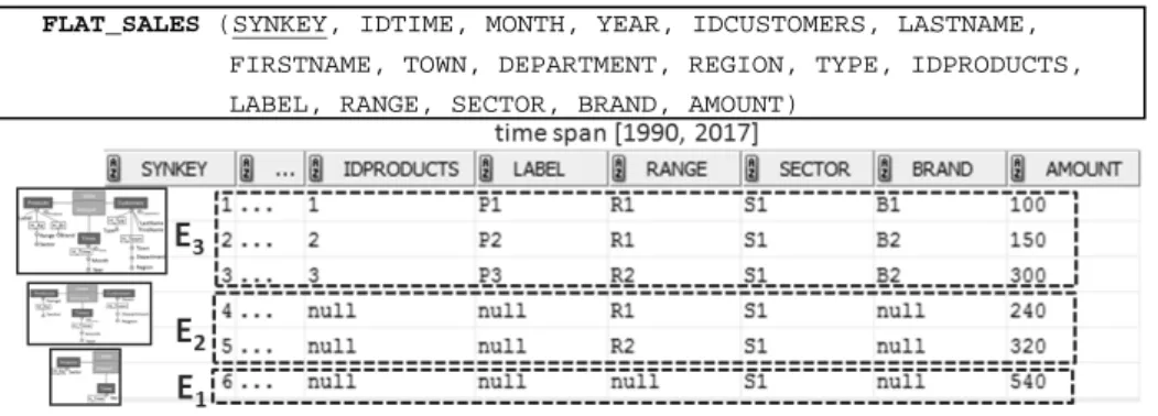
FLAT_SALES (SYNKEY, IDTIME, MONTH, YEAR, IDCUSTOMERS, LASTNAME, FIRSTNAME, TOWN, DEPARTMENT, REGION, TYPE, IDPRODUCTS, LABEL, RANGE, SECTOR, BRAND, AMOUNT)

A snapshot1 of instances in the flat table is shown in the figure 2. Instances from the latest state E3 are directly loaded in the flat table (cf. lines 3 and 10), while the

other two states E2 and E1 are loaded with NULL value as placeholder for the deleted

attributes' instances (cf. lines 3-6 and 10).

3.3 Horizontal modeling of a reduced MDB

The second relational modeling alternative is named horizontal. Each state is imple-mented through a fact table and a set of dimension tables. The algorithm of the

hori-zontal modeling is as follows.

Algorithm 2. Horizontal Modeling

Input: a reduced MDB composed of a set of states E = {E1; …; En}.

Outputs:

─ a set of fact tables TFact={TF₁; …; TF_n}, such as ∀TF_i∈TFact, TF_i=(SynKeyi, FKey_i,

M_i) implements the fact Fi of the state Ei, where SynKeyi is a synthetic primary

key; FKey

i is a set of foreign keys; Mi is a set of measures in TFi.

─ a set of dimension tables TDim={T_D 1 E1; …; T_D w En}, such as ∀T D_jEi∈TDim, T_D j Ei= (Key_Tji, A_T

ji) implements the dimension Dj of the state Ei, where KeyTji is a primary

key of the dimension table; A_T

ji is a set of attributes.

Begin

1. For each state Ei∈E, Ei={Fi; Di; Ti}

2. Create a fact table T_Fi = (SynKeyi, FKey_i, Mi), where FKey_i←∅, Mi←MFi;

3. For each dimension Dj∈Di

4. Find the parameter p1 on the lowest granularity of Dj ;

5. _FKey

i←FKeyi∪{p1};

6. Create a dimension table T

D_jEi=(KeyTji, AT_ji), set KeyTji←p1, A_Tji←ADi\{p1};

7. Insert attribute instances within Dj into T_D j Ei; 8. End for

9. Insert measure instances within Fi with related parameter instances into TF_i

10. End for End

The horizontal modeling creates a fact table T_Fi for each state Ei. Each fact table

includes all measures from the fact Fi and a set of foreign keys (cf. lines 1 and 2).

Each foreign key consists of the parameter on the lowest granularity of a dimension from the state Ei (cf. line 5). Each dimension Dj is converted into a dimension table as

follows: the parameter p1 of the lowest granularity on Dj is used as a primary key,

while other attributes on the dimension (i.e. ADi\{p1}) are directly added in the

dimen-sion table (cf. lines 3-6). Consequently, the time span of a fact table and a dimendimen-sion table corresponds to the temporal interval of the involved state.

1

For the sake of simplicity, all snapshots in this section include only the dimension Products.

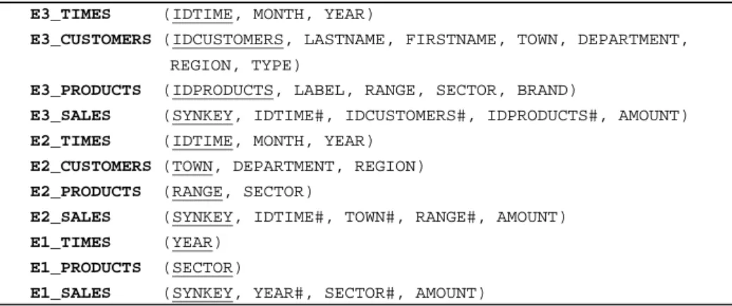
Example. According to the algorithm 2, the reduced MDB of the case study is im-plemented through 3 fact tables and 8 dimension tables.

E3_TIMES (IDTIME, MONTH, YEAR)

E3_CUSTOMERS (IDCUSTOMERS, LASTNAME, FIRSTNAME, TOWN, DEPARTMENT, REGION, TYPE)

E3_PRODUCTS (IDPRODUCTS, LABEL, RANGE, SECTOR, BRAND)

E3_SALES (SYNKEY, IDTIME#, IDCUSTOMERS#, IDPRODUCTS#, AMOUNT) E2_TIMES (IDTIME, MONTH, YEAR)

E2_CUSTOMERS (TOWN, DEPARTMENT, REGION) E2_PRODUCTS (RANGE, SECTOR)

E2_SALES (SYNKEY, IDTIME#, TOWN#, RANGE#, AMOUNT) E1_TIMES (YEAR)

E1_PRODUCTS (SECTOR)

E1_SALES (SYNKEY, YEAR#, SECTOR#, AMOUNT)

Figure 3 displays a snapshot of instances in the reduced MDB implemented ac-cording to the horizontal modeling.

Fig. 3. A snapshot of instances organized according to the horizontal modeling

3.4 Vertical modeling of a reduced MDB

The third alternative is named vertical modeling. It gathers common components among states into separate tables called vertical tables. Each vertical table includes measures and attributes shared by some states. We propose the following algorithm for the vertical modeling.

Algorithm 3. Vertical Modeling

Input: a reduced MDB composed of a set of states E = {E1, …, En}.

Output: a set of vertical tables TV={T_V1, …, T_Vn}, such as ∀T_Vi∈TV, T_Vi={SynKey_i,

A_i, M_i} is a vertical table for a subset of states, where SynKeyi is a synthetic key; A_i is

a set of attributes; M_i is a set of measures. Begin

1. For each i from 1 to n (n=|E|)

2. Create a vertical table T_Vi={SynKey_i, A_i, M_i}, where ─ A_i←⋃_D ADk

k∈Di such as Di is the set of dimensions from the state Ei;

3. For each Ex∈E

4. Insert into T_Vi instances of attributes A_i; 5. Insert into T_V

i aggregated values of measures Mi from Ex according to A_i;

6. End For 7. E←E\{Ei};

8. End for End

According to the definition of the data reduction, attributes and measures from an old state Ei must exist in a more recent state Ej (i<j). Therefore, to gathers common

components in a subset of states {Ei, …, En} (1≤i≤n), the ith vertical table TV_i groups

together attributes and measures from the ith state (cf. lines 1 and 2). Then, for each state Ex in {Ei, …, En}, instances of each attribute in A_i are retrieved from the state Ex

and then loaded in T_Vi. Based on the attribute instances, values of each measure in M_i from Ex are aggregated and then inserted into TV_i (cf. lines 3-6). Consequently, each

vertical table T_Vi covers a time span from the state Ei to the latest state En.

Example. After applying the algorithm 3 to our case study, we obtain the follow-ing three vertical tables.

VTABLE1 (SYNKEY, YEAR, SECTOR, AMOUNT)

VTABLE2 (SYNKEY, IDTIME, MONTH, YEAR, TOWN, DEPARTMENT, REGION, RANGE, SECTOR, AMOUNT)

VTABLE3 (SYNKEY, IDTIME, MONTH, YEAR, IDCUSTOMERS, LASTNAME, FIRSTNAME, TOWN, DEPARTMENT, REGION, TYPE, IDPRODUCTS, LABEL, RANGE, SECTOR, BRAND, AMOUNT)

The snapshot presented in figure 4 indicates a state of reduced MDB is implement-ed through one or several vertical tables. For instance, data from the latest state E3 are

found within all vertical tables: (i) VTABLE3 includes the sale amount from 2010 to 2017 by IDProducts; (ii) VTABLE2 aggregates the amount from the state E3

accord-ing to products' range; (iii) VTABLE3 further aggregates the amount from the state E3

according to product's sector.

3.5 Comparison among relational modeling alternatives

A conceptual reduced MDB can be transformed into various relational schemas. Ex-tracting the same data requires applying different queries to different relational sche-mas with different data redundancy ratios.

The flat modeling consists of a simplistic way which converts the whole reduced MDB into one relation. It frees queries from joins, regardless of the number of in-volved dimensions. However, the flat modeling causes high data redundancy: attrib-ute instances are repetitively stored in the relation with related measure instances.

The horizontal modeling is a more complex method which converts measures and attributes from one state into independent relations. It minimizes data redundancy by associating attribute instances with related measure instances through primary key -

foreign key relationships. However, the horizontal modeling requires joins in queries

involving dimension tables.

The vertical modeling converts measures and attributes shared by several states in-to separate relations. This modeling has multiple advantages. On one hand, queries involving several dimensions do not have to include joins. On the other hand, data redundancy is reduced to attribute instances within some high levels on dimensions.

To accurately and quantitatively study the influences of different relational model-ing alternatives on query execution efficiency, the remainder of this paper focuses on some experimental assessments.

4

Experimental assessments

In this section, we carry out some experimental assessments by executing queries in reduced and unreduced MDBs populated with data according to different volumes.

4.1 Protocol

The objective of our experimental assessments is twofold: (i) studying if all relational modeling alternatives for reduced MDBs help improving query execution efficiency and (ii) identifying the most efficient relational modeling of reduced MDBs. Existing multidimensional data benchmarks (e.g. TPC-DS2 and SSB[9]) are designed to meas-ure a system's performance [3]. They do not allow testing the effect of different re-duced modeling solutions, since the included MDB is composed of only one state.

Facing this issue, we have to generate our own test data during the experimental assessments. The MDB of our case study is used and populated with synthetic data. Three reduced MDB implementations, namely flat, horizontal and vertical, are built according to the relational modeling alternatives (cf. section 3). Two unreduced MDBs are used as baseline to assess the impact of data reduction: (i) the unreduced

flat MDB integrates all attributes and measures before reduction into one table and (ii)

the unreduced horizontal MDB includes one fact table and three dimension tables

2

http://www.tpc.org/tpcds/

without reduction. The number of tuples as well as redundancy ratio of attribute in-stances according to MDB implementation and scale factor is shown in table 1.

Table 1. Scale factors and number of tuples with attribute instance redundancy ratio.

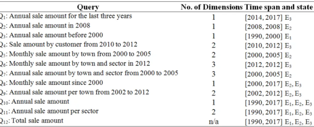
During the experimental assessment, we consider only queries producing full an-swers in MDBs before and after data reduction. Meanwhile, different queries should involve different dimensions in different states during querying. Table 2 shows our proposed 12 queries. Specifically, queries Q1-Q3 involve one dimension in one state;

queries Q4-Q7 involve multiple dimensions in one state; queries Q8 and Q9 involve

different dimensions in two states; Q10-Q12 involve different dimensions in all states.

Table 2. 12 queries involving different dimensions and time spans.

For each query, we record the execution costs provided by the Explain Plan com-mand of the Oracle 12c DBMS without any optimization techniques (e.g. index and table partitioning). The hardware configuration is as follows: 2×[email protected] with 2 cores, 128GB RAM and 1TB SSD Disk in RAID6.

4.2 Observations and discussions

In this section, we study the query execution costs in reduced and unreduced MDBs of different scale factors.

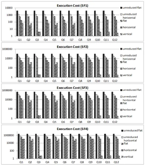
Observation. From figure 5, we can see the same trend is found in MDBs of ferent scale factors. The lowest execution costs of the twelve queries come from dif-ferent implementations of reduced MDB. Specifically, for queries covering a time span within the temporal interval of one state, regardless of the scale factor and the number of dimensions included, (i) the lowest execution costs of Q1, Q4 and Q6

(with-in the temporal (with-interval of E3) are found within the vertical MDB; (ii) the lowest

exe-cution costs of Q2, Q5 and Q7 (within the temporal interval of E2) are produced by the

horizontal MDB; (iii) both the vertical and the horizontal MDBs are cost-efficient for

Q3 (within the temporal interval of E1). All queries involving multiple states are more

efficiently computed within the vertical MDB (from Q8 to Q12), regardless of the MDB volume and the number of states as well as dimensions involved.

Fig. 5. Query execution costs in reduced and unreduced MDBs of different scale factors Discussion. Based on the above observations, we can conclude that regardless of the scale factor, reduced MDBs always produce lower execution costs than unreduced MDBs. The execution costs in reduced MDBs (i) are not significantly influenced by the number of dimensions involved in a query but (ii) highly depend on the time span involved in a query. The more a query and a reduced MDB implementation share in terms of time span, the lower the execution costs become. When a query only

in-volves old states, the influence of time span is weakened by the small volume of data within the horizontal and the vertical MDBs.

Fig. 6. Average execution costs by query type and MDB implementation of SF1 Observation. Figure 6 shows the average query execution costs in MDBs of the scale factor SF1 according to query type. No matter how many states are involved in que-ries, the average execution costs in reduced MDBs are always lower than in unre-duced MDBs. The highest average execution costs are found within the unreunre-duced

flat MDB, while the lowest one is obtained by the vertical MDB. Comparing with

unreduced MDBs, reduced MDBs significantly decrease the execution costs: from 54.4.% to 98.96%.

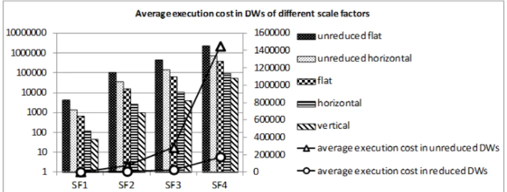
As we can see from figure 7, the same trend is found in MDBs of larger scale fac-tors. From the unreduced flat MDB to the vertical MDB, the average execution costs decrease significantly: over 100 times (cf. the vertical axis on the left in figure 7). Moreover, the differences between the average execution costs in unreduced and re-duced MDBs keep increasing as the data volume grows; i.e. from SF1 to SF4, the gap has widened about 513 times (cf. the vertical axis on the right in figure 7).

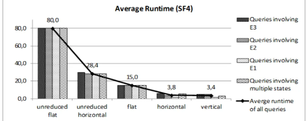
Fig. 7. Average execution costs of all queries in MDBs of different scale factors In reduced MDBs, the decrease in execution costs is directly reflected in the gain in query runtime. Figure 8 shows the average runtime in MDBs of the scale factor 4 according to query type.

Discussion. All reduced MDBs allow significantly saving the query execution costs, regardless of the scale factor and the query type. More importantly, the results of our experimental assessments show the scalability of our proposal: the larger the

MDB is, the more significant the decrease in execution costs becomes after data re-duction. The most efficient relational modeling is the vertical MDB. It groups meas-ure instances and related attribute instances from one state together and implements them in one table. Consequently, data redundancy is reduced, while queries involving multiple dimensions are freed from joins in a vertical reduced MDB.

Fig. 8. Average runtime of queries involving different states in the largest MDBs

5

Conclusion

Our aim is to support effective and efficient decision-making by storing only data of high informative value over time in a MDB. In this paper, we outline a conceptual modeling solution allowing reducing both facts and dimensions in MDBs. A reduced MDB is modeled with multiple states. Each state is valid for a period of time.

Three relational modeling alternatives are proposed for reduced MDBs. The flat modeling integrates all measures and attributes from all states into one single flat table. The horizontal modeling converts each state into a fact table and a set of di-mension tables. The vertical modeling gathers common measures and attributes shared by states into vertical tables. Different relational modeling alternatives (i) re-quire different numbers of joins in analysis queries and (ii) bring in different degrees of information redundancy.

We carry out some experimental assessments to evaluate query execution efficien-cy in reduced and unreduced MDBs. The result shows the data reduction is a scalable solution: the larger the MDB is, the more significant the improvement in query execu-tion efficiency becomes after the data reducexecu-tion. During our experimental assess-ments, the improvement in terms of query execution costs ranges from 54.4.% to 98.96%. The most significant decrease in query execution costs is found in the

verti-cal MDB, which makes it the most efficient relational modeling of reduced MDBs.

In the future, we intend to study the performance of our proposed relational model-ing alternatives in other types of DBMS. As more and more NoSQL systems nowa-days are adopted to deal with large amount of data, it would be necessary to study new data reduction strategies in the context of NoSQL. One of our ongoing work focuses on reducing data in graph databases and triple store (RDF) databases.

6

References

1. Atigui F, Ravat F, Song J, Teste O, Zurfluh G (2015) Facilitate Effective Decision-Making by Warehousing Reduced Data: Is It Feasible? Int J Decis Support Syst Technol 7:36–64. 2. Berkani N, Bellatreche L, Benatallah B (2016) A Value-Added Approach to Design BI

Applications. In: Madria S, Hara T (eds) Big Data Anal. Knowl. Discov. pp 361–375 3. Darmont J, Bentayeb F, Boussaid O (2007) Benchmarking data warehouses. Int J Bus

Intell Data Min 2:79–104. doi: 10.1504/IJBIDM.2007.012947

4. Garcia-Molina H, Labio W, Yang J (1998) Expiring data in a warehouse. In: 24rd Int. Conf. Very Large Data Bases. Morgan Kaufmann Publishers Inc., New York, pp 500–511 5. Golfarelli M, Maio D, Rizzi S (1998) Conceptual design of data warehouses from E/R

schemes. In: Thirty-First Annu. Hawaii Int. Conf. Syst. Sci. IEEE Computer Society, Kohala Coast, HI, pp 334–343

6. Iftikhar N, Pedersen TB (2011) A rule-based tool for gradual granular data aggregation. In: Int. Workshop Data Warehous. OLAP. ACM Press, Glasgow, United Kingdom, pp 1–8 7. Nebot V, Berlanga R, Pérez JM, Aramburu MJ, Pedersen TB (2009) Multidimensional

In-tegrated Ontologies: A Framework for Designing Semantic Data Warehouses. In: J. Data Semant. XIII. Springer Berlin Heidelberg, pp 1–36

8. Okun O, Priisalu H (2007) Unsupervised data reduction. Signal Process 87:2260–2267. doi: 10.1016/j.sigpro.2007.02.006

9. O’Neil P, O’Neil E, Chen X, Revilak S (2009) The Star Schema Benchmark and Aug-mented Fact Table Indexing. In: Perform. Eval. Benchmarking. Springer Berlin Heidel-berg, Berlin, HeidelHeidel-berg, pp 237–252

10. Skyt J, Jensen CS, Pederson TB (2002) Specification-based data reduction in dimensional data warehouses. IEEE Comput. Soc, p 278

11. Udo IJ, Afolabi B (2011) Hybrid Data Reduction Technique for Classification of Transac-tion Data. J Comput Sci Eng 6:12–16.