Any correspondence concerning this service should be sent
to the repository administrator:
[email protected]
This is an author’s version published in:
http://oatao.univ-toulouse.fr/27268
To cite this version: Di Pretoro, Alessandro
and Montastruc,
Ludovic
and Manenti, Flavio and Joulia, Xavier
Exploiting
Residue Curve Maps to Assess Thermodynamic Feasibility Boundaries
under Uncertain Operating Conditions. (2020) Industrial &
Engineering Chemistry Research, 59 (36). 16004-16016. ISSN
0888-5885
Official URL
DOI :
https://doi.org/10.1021/acs.iecr.0c02383
Open Archive Toulouse Archive Ouverte
OATAO is an open access repository that collects the work of Toulouse
researchers and makes it freely available over the web where possible
Exploiting Residue Curve Maps to Assess Thermodynamic Feasibility
Boundaries under Uncertain Operating Conditions
Alessandro Di Pretoro, Ludovic Montastruc,
*
Flavio Manenti, and Xavier Joulia
ABSTRACT: The veryfirst step of almost any separation process design procedure is the thermodynamic feasibility analysis. In the case of distillation, residue curve maps (RCMs) represent an essential tool to assess whether the separation is feasible or not. However, the analysis is generally carried out by referring to nominal operating conditions and product purities as specification. This means that, when process parameters are likely to undergofluctuations, the prediction of the system response is not that obvious. An ABE/W (acetone−butanol−ethanol/water) mixture was then selected as a case study since it allows us to discuss several non-ideal thermodynamic behaviors and because of the renewed interest in biorefinery and sustainable processes during recent years. Residue curve mapping was then exploited to determine the thermodynamic feasibility range for multicomponent distillation processes as well as for distillation trains and process-intensified solutions taking into account both product purity and product recovery specifications. The final product of this study is a thorough procedure to determine the flexibility boundaries of feed and product compositions as well as an immediate and intuitive graphical representation from a binary standard distillation column to a complex multicomponent dividing wall column application.
■
HIGHLIGHTS(1) An a priori thermodynamic flexibility assessment could avoid a backward investigation on the system unfeasibility root causes when perturbations occur. (2) Biofuel purification is a challenging operation due to the
high non-ideality of water-alcohols interactions and the seasonality of the feedstock.
(3) Residue curve mapping has proved to be an effective methodology worth exploited even when uncertainty should be taken into account.
2. INTRODUCTION
Feasibility analysis is a key point and the veryfirst step of any process design procedure independent of the process nature. It is usually carried out according to given operating conditions in order to proceed to the following design phases. After the solution to the initial problem has been preliminarily designed, it is usually tested by varying design variables or
operating parameters.1 However, whether the process results to be unfeasible, it could be very difficult to understand, which is the constraining aspect that prevents the operation to achieve the desired specifications. The inability of a system to withstand operating conditions different from the ones according to which it has been designed indeed can be either due to tight constraints, such as physical laws, or loose constraints, such as available materials or design choices.2 In the latter case, those limitations can be usually overcome by means of higher investments or at the cost of a lower profitability. On the contrary, in the former cases, it does not
exist in any way to bypass the system failure, and a different design solution should be employed. Moreover, in all those cases, an a priori thermodynamicflexibility assessment would have avoided the backward investigation on the unfeasibility root cause.
These considerations are obviously dependent on the uncertain variable deviation range as well as the deviation likelihood.1 The petrochemical industry for instance is based on widely studied and well-established processes, and crude oil supplies are ruled by multiyear contracts involving oil blends whose properties are known and are almost constant in time. However, the growing interest toward sustainable feedstocks during recent years implies considerable mod-ifications in the process design approach. The biomass nature indeed is ruled by the cycle of seasons and cannot ensure constant chemicophysical properties during the year;3,4 this causes the definition of “nominal operating conditions” to be of little significance and an a priori design under uncertainty to be extremely useful.
A relevant part of biobased processes indeed involves the use of a fermenter upstream the product separation section; the obtained fermentation broth is rich in water and alcohols in prevalent quantities that were not that present in petroleum feedstocks and considerably complicate the thermodynamic behavior due to the high non-ideality of their interactions. It would not be then surprising if, during an operation, an external operating condition perturbation or malfunctioning of an upstream unit led the separation section conditions outside the feasibility boundaries with relevant implications on the delicate profitability of a fermentation process.
Among the most common operations in chemical plants, distillation is by far the most used and the one processing huge feedstock capacities. It involves relatively high energy costs and its separation effectiveness is of critical importance for the cost-effectiveness of the entire process.
For all these reasons, this study deals with the thermodynamic flexibility assessment of different typologies of distillation processes involving compounds coming from an upstream microbial fermentation process as thoroughly described in the following chapters.
3. METHODOLOGY
Distillation feasibility is a widely spread and deeply studied research domain since the very beginning of the 20th century. Several methodologies exist in order to assess whether a given mixture split is possible or not on the basis of the components’ volatility. Some shortcut methods have been outlined as well for the preliminary design phase accounting for a constant relative volatility between the species and the heavy−light key components’ assumption. However, when thermodynamics gets complicated, equilibrium diagrams are the reference to be employed. A useful and well-established tool to assess the thermodynamic feasibility of a multi-component mixture distillation process based on equilibrium diagrams is residue curve mapping. Despite the robust theory behind them and their effective graphical representation allowing for an immediate understanding of the equilibrium phenomena, residue curve maps (RCMs) are seldom used as the main tool to show the feasibility study results by process engineers.
Those curves were defined first at the beginning of the 20th century by Ostwald (1900)5 and Schreinemakers (1901)6 in Germany to describe ternary mixtures with the presence of
azeotropic species. However, the country where they have seen the highest development after approximately 50 years is Russia; Gurikov (1958)7 indeed classified all the possible ternary diagrams and Zharov and Serafimov8−12 completed their work for mixtures with a higher number of components. All those studies remained untranslated from Russian for a long time.
The main research work concerning residue curves during recent years was performed by Petlyuk,13,14and it will be the mainly referenced author in this chapter. The residue curve represents the evolution of the mixture composition during the open evaporation process as shown inFigure 1.
From a numerical point of view, the mass balance on the ith component can be reconducted, in correspondence to each infinitesimal amount of the vaporized mixture dL → 0, to the differential equation: ξ = − x x y d d i i i (1)
where dξ represents the infinitesimal dimensionless time span, i.e., the evaporation extent.
A residue curve is then given by the locus of points in the composition domain satisfying the ordinary differential equation corresponding to a certain moment of time and to a portion of evaporated liquid.
Another physical interpretation that could result to be more appealing from a practical point of view concerns distillation columns. In particular, at total reflux, composition profiles of packed columns are described by residue curves, whereas distillation lines coincide with the composition profiles of staged columns.15
A close correspondence between RCMs and distillation trajectories at infinite reflux was also proved. Distillation trajectories represent the composition profile along the column equilibrium stages; at infinite reflux, as first discussed by Thormann,16they are given by
= = ̅ ̅ ·
+
xi(k 1) yi( )k K Ti( ( )k,P( )k,x( )k,y( )k)xi( )k (2)
If we interpolate those broken lines with a continuous one, the so-called distillation c-lines can be obtained. Distillation lines and (equilibrium) tie-line curves are a unique function of the vapor−liquid equilibrium, independent of their analogies with the column composition profile. Thus, distillation lines are equivalent to residue curves as characteristics of the VLE in a thermodynamic sense although they do not coincide as discussed by Kiva et al. (2003).17
Residue curves indeed are oriented curves; they move from the unstable node that is the light component or azeotrope (the star inFigure 2a,b) to the stable node that is the heavy component or azeotrope (the square inFigure 2a,b) passing
more or less close to an eventual saddle point representing the compound or species with an intermediate volatility (the circle inFigure 2a,b).
Whenever two or more distillation bundles are present, except for binary distillation, one or more particular residue curves called “separatrices of saddle stationary points” delimiting them exist as well. Different from the other RCs, the separatrices begin or come to an end not in the node points but in the saddle points (cf.Figure 2b). They separate two distillation regions, i.e., concentration bundles where all RCs have the same stable and unstable nodes in common. The main outcome related to the analysis of distillation regions is that separatrices cannot be crossed, which means that we cannot move between two points belonging to different distillation regions during a single distillation process. In the light of the above, the important conclusion that can be drawn is that, in order to be part of the same distillation column, the characteristic points representing lateral feeds and product withdrawals should therefore have the same stable and unstable nodes, i.e., the RCs passing through them should belong to the same distillation region. This is a rule of general validity with the exception of a few particular cases when the VLE equilibrium behavior exhibits a nonideality resulting in inflections of the total reflux trajectories. Those cases are not specifically treated in this study, but a more accurate discussion can be found in Wahnschafft et al. (1992)18 and Petlyuk (2004).14
Thus, thefirst goal of this study is to take advantage of the RCM theory robustness in order to discuss distillation of complex multicomponent mixtures under uncertain operating conditions, i.e., theflexibility range of the operation. Flexibility will be evaluated according to the resilience index introduced by Saboo et al. (1985)19 defined as the largest total disturbance load independent of the direction of the disturbance, a system able to withstand without becoming unfeasible.
An additional purpose of this study is then to provide graphic tools to ease the understanding of the multi-component mixtures’ behavior both for a single distillation column and for more complex distillation configurations using the product purity and its recovery ratio as specifications.
Calculations have been performed by coupling Matlab for the numerical and graphical part with Simulis
Thermody-namics software providing the component databank as well as the thermodynamic models and parameters.
4. CASE STUDY
It is widely agreed that sustainability can be identified as the worldwide central issue of the last (and the next) several years. According to the IEA Bioenergy Annual Report,20 biofuels will represent around 30% of energy consumption in transport by 2060. Their role is particularly important in sectors that are difficult to decarbonize, such as aviation, shipping, and other long-haul transport. That is why several bioprocesses have seen renewed interest in recent years both from a research and an industrial point of view.
For this reason, the ABE/W (acetone−butanol−ethanol/ water) mixture was selected as the case study analyzed in this paper. It comes from an upstream microbial fermentation process characterized by product inhibition21and the recovery of at least the most valuable products, n-butanol and acetone, is necessary for the profitability of the process. After a preliminary dewatering operation, usually liquid−liquid extraction or pervaporation,22−24the remaining products can be separated by means of different distillation configurations. The fluctuation related to the feedstock nature requires a dedicated design procedure taking into account the inlet composition uncertainty and aiming to a flexible design choice.
An additional reason why this multicomponent mixture is particularly suitable for this flexibility assessment is that the complex and highly non-ideal thermodynamics allows us to analyze interesting singular points such as homogeneous and heterogeneous azeotropes as well as to include liquid−liquid equilibrium in the distillation feasibility assessment and optimization discussion thanks to the aqueous−organic phase demixing.
From the most significant binary case studies to more complex multicomponent mixtures, both simple distillation and energy integrated configurations will be discussed by referring to these four compounds.
The process specifications accounted for in the case of a single distillation column are
(1) n-Butanol recovery ratio in the bottom: 0.9604. (2) Bottom n-butanol mass fraction: 0.99.
In the case of the water−ethanol mixture, the recovery specifications will be applied to water since, in order to obtain high-purity ethanol with a single distillation column, the feed composition should be at least 95.63% w/w pure (azeotropic composition) with a consequent poor flexibility interest.
More realistic specifications for the ethanol-water separation will be considered as listed here below:
(1) Water recovery ratio in the bottom: 0.95. (2) Bottom water mass fraction: 0.95.
Furthermore, in the case of two distillation columns or a dividing wall column, the following constraints should be included in addition to the n-butanol ones:
• Acetone recovery ratio in the distillate: 0.985. • Distillate acetone mass fraction: 0.995.
The single distillation column case studies will be then discussedfirst, and the distillation trains as well as the DWC case studies will be presented at the end of the following chapters. All the distillation columns presented in this paper will refer to an atmospheric operating pressure.
The most suitable thermodynamic model to describe the ABE/W mixture equilibrium behavior is the non-random two liquids (NRTL).25 It results indeed to be the most accurate model able to describe water−alcohols as well as biofuel equilibria in general.24,26−28
5. THE BINARY SYSTEMS
Among the six possible binary systems of an ABE/W mixture, two in particular have been selected to conduct theflexibility limit analysis, namely, the water−ethanol and water−butanol mixtures. Thefirst reason of this choice was that it would be obviously meaningless to analyze mixtures with no saddles, e.g., acetone−ethanol, since it is always possible to perform a sharp separation by distillation with an infinite number of stages (that is the characteristic condition of RCMs). The second reason why it is worth discussing these two mixtures is that they allow us to show analogies and differences between homogeneous and heterogeneous azeotropes, i.e., whether the liquid phase can undergo demixing or not.
In a two-component system, the residue curve moves from the unstable to the stable node along a 1-D trajectory, i.e., the liquid phase composition curve. Since distillation regions for N component mixtures are N − 1 dimensional spaces, in a binary system, the distillation region is part of the x1domain. The following chapter will then concern the well-known water−ethanol equilibrium under a flexibility perspective; after that, a chapter related to the water−butanol binary system will be presented to show how introducing an additional operation different from distillation will affect the residue curve shape and theflexibility of the separation.
5.1. Homogeneous Azeotrope. Among all binary mixtures showing a feasibility limit, water−ethanol is by far the most popular due to its several uses and its ancient history. At atmospheric pressure, this mixture presents a minimum boiling point azeotrope at 78.2 °C and an ethanol composition of 95.63% w/w corresponding to approximately 89.5% mol/mol.29
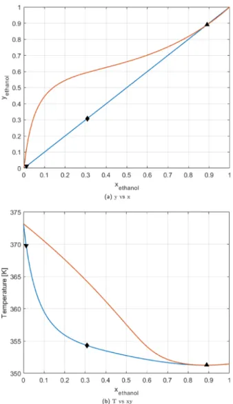
The y versus x and T versus xy equilibrium diagrams are reported inFigure 3a,b respectively. As it can be noticed, the residue curves, i.e., the composition of the residual liquid phase, in a binary plot are just represented by the diagonal of the y versus x diagram (since they correspond to the column profile at infinite reflux) or by the bubble curve in T versus xy.
The azeotrope divides then the 1-D space into two distillation regions, xethε[0,0.895] and xethε[0.895,1]. In the first
distillation region, the sharp split that can be obtained is pure water as a bottom product and at the azeotropic composition as a distillate product; in terms of residue curve vocabulary, it can be stated that pure water is the stable node and the azeotrope is the unstable node in thefirst distillation region, while, in the second distillation region, the azeotrope is still the unstable node but pure ethanol becomes the stable one.
Therefore, since 0.95 w/w water purity is desired, the first trivial conclusion can be immediately drawn: the feed ethanol molar fraction should be lower than the azeotropic one, i.e., the operating line will lie on the left side of the equilibrium diagram. The operating point corresponding to the bottom product is fixed according to the given specification xethw =
0.05 (xethmol= 0.02).
The other constraint related to the recovery ratio affects the feed split into the distillate and bottom streams; this coincides, from a geometrical point of view, with the application of the so-called lever rule:
̅ − ̅ ̅ − ̅ = z x x z D B B D (3)
Figure 3.(a, b) Ethanol−water equilibrium diagrams: solid inverted triangle - bottom, solid diamond - feed, and solid triangle - distillate.
Therefore, for any given feed composition, the bottom point location is fixed by means of the bottom composition specification, and the distillate point can be located by taking into account the mass balance.
With the exception of particular cases, the necessary and sufficient conditions to state that a separation by distillation is possible is that the feed, distillate, and bottom composition points lie in the same distillation region, i.e., they all should have the same stable and unstable nodes (for further details about the theoretical background, please refer to Petlyuk (2004)14). In the case of binary distillation, then, they all should lie on the same side of the azeotrope.
By applying these rules to the ethanol−water case study under analysis, it can be deduced that the maximum ethanol content in the feed stream is the one for which the distillate characteristic point lies on the distillation region boundary (xethD = xethazeo= 0.895). Thus, to satisfy the process specification
(the water recovery ratio in the bottom equal to 0.95), the maximum ethanol molar fraction in the feed is zeth= 0.308. It
means that, if the process operating conditions correspond to a lower value, there is aflexibility range zethε[0,0.308] within which the feed ethanol content can fluctuate without compromising the desired separation feasibility with a single distillation column. On the contrary, if the feed composition perturbations above the limit value can be attained, the thermodynamic feasibility boundary is breached and there is no way to achieve the process specifications no matter the investment that we would be willing to afford; in those cases, the only solution is to design a different separation process.
In conclusion, it is worth remarking that, although this result is strictly related to the process specifications, the same methodology can be nevertheless applied to any distillation case study.
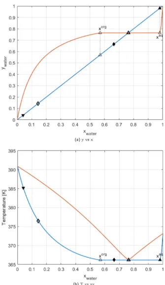
5.2. Heterogeneous Azeotrope. Though, atfirst glance, the water−butanol mixture could look similar to the water− ethanol one, it needs a considerably different procedure. Indeed, the main difference can be immediately noticed by means of the equilibrium diagrams inFigure 4a,b. If making the assumption of simple distillation (no decanter), the operating points are represented by the solid markers (inverted triangle for the bottom, diamond for the feed, and triangle for the distillate). Even for this case study, the heteroazeotrope xwatazeo= 0.76328divides the 1-D space into two
distillation regions, xwatε[0,0.763] and xwatε[0.763,1], and it is
the unstable node for the region on the left-hand side (pure n-butanol, heteroazeotrope) as well as for the region characterized by the heteroazeotrope-pure water split. Then, in order to obtain pure butanol with the desired recovery ratio, the feed stream should be located on the left of the heteroazeotrope.
The thermodynamic flexibility problem can then be solved analogously to the water−ethanol mixture (Figure 5left); the bottom stream molar fraction isfixed according to the purity specification, the lever rule can be applied according to the recovery ratio, and, with the maximum water content in the distillate being xwatD = xwatazeo = 0.763, the maximum water
content in the feedflow rate results to be zwat = 0.1434.
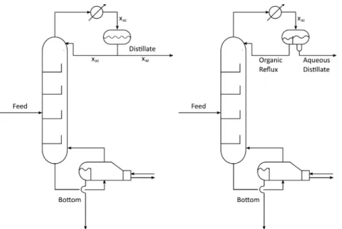
However, in the case of the heterogeneous azeotrope, there is a well-established column configuration30 aimed at increasing the operation effectiveness based on the use of a decanter instead of a conventional reflux drum (cf. Figure 5 right). For the analysis we are trying to carry out, the addition
of a decanter implies considerable modifications worth discussing before providing the corresponding results.
First of all, the distillation column with a decanter as a reflux drum (as shown in Figure 5 right) has one degree of freedom less with respect to the standard configuration since the reflux flow rate is a direct consequence of the equilibrium demixing and cannot be managed by a dedicated control system to achieve a desired specification. Thus, the separation problem should be differently posed: for a given feed flow rate, indeed, either the butanol purity or the butanol recovery ratio can be imposed. This means that one process specification must be loosened and transformed from equality into inequality constraint. It can then be stated that a 99% w/ w purity is required and an n-butanol recovery ratio must be equal to at least 0.9604.
The second main difference between the two configurations concerns the overcooling degree in the condenser. In the standard distillation column, the reflux overcooling is unprofitable because it involves higher-duty requirements both in the condenser and reboiler since a liquid phase further from the equilibrium conditions is recycled without affecting the distillate (and then the reflux) composition. On the contrary, when demixing occurs, the aqueous and organic
Figure 4. (a, b) n-Butanol−water equilibrium diagrams: solid inverted triangle - bottom, solid diamond - feed, and solid triangle - distillate.
phase compositions depend on temperature. The water content of the distillate stream can be then modified according to the overcooling degree enhancing the separation with a relatively poor cost increase since the condenser temperature allows the use of ambient water as a cooling duty. However, as evidenced by well-established experimental data,31,32 the aqueous phase composition in the temperature range [0°C, 91 °C] can only vary from 0.9727 to 0.9838 with an xwataq = 0.98 value at the boiling point without considerably
affecting the thermodynamics of the system. On the contrary, the water content in the organic reflux can significantly change; even though this parameter could improve the separation efficiency from an energetical point of view due to the fact that a lower amount of water circulates through the column, it does not modify the separation thermodynamic feasibility since the reflux stream does not take part in the overall mass balance. For all these reasons, the thermody-namic feasibility analysis has been carried out without condenser overcooling.
The residue curve analysis results can be noticed inFigure 4a,b by referring to the solid markers (diamond for the feed and triangles for the bottom and distillate). The distillate water molar fraction shifted from xwatD = xwatazeo= 0.763 to xwatD =
xwataq = 0.98 with a relevant increase of the maximum water
content allowed in the feed stream to zwatmax= 0.6647.
Note that, if the feed composition is included in the range [xwatorg,0.6647], it is worth feeding directly in the condenser in
order to take advantage of the feed demixing and reduce the amount of water introduced in the column as discussed in the work of Luyben (2008).30
The trend of the butanol recovery ratio in the bottom stream is represented inFigure 6in the range zwatε[xwatB , z
wat max].
It can be noticed that the butanol recovery specification is satisfied for any water content in the feed lower than the maximum value.
6. MULTICOMPONENT SYSTEMS
Process feedstocks are usually composed of several different components even though sometimes only a few of them are worth recovering. Multicomponent mixtures equilibria can be
visualized by means of a multiphase diagram. The diagrams’ dimensionality is related to the number of compounds, namely, N component mixtures require an (N − 1) D diagram. For this reason, the thermodynamic flexibility assessment procedure will be graphically discussed here below up to four components, i.e., the limit of a 3D representation. These diagrams allow nevertheless the ABE/W mixture behavior analysis. The procedure explained in the following paragraphs is nonetheless of general validity independent of the number of mixture components. The analytical procedure in the case of an N higher than 4 is discussed in a dedicated chapter at the end of this section.
The mixture water content will still be used as an uncertain variable since it has been revealed to be the most critical parameter for the separation.
6.1. Ternary System. Since butanol−water and ethanol− water binary mixtures have been analyzed in the previous chapter, the ternary mixture butanol−ethanol−water obtained combining them will be discussedfirst while acetone will be added later as the fourth compound.
It is worth remarking that we are still dealing with a single distillation column whose specifications are related to the
n-Figure 5.Standard distillation column vs distillation column with a decanter.
butanol recovery and purity as discussed in Section 4, Case Study.
Nominal operating conditions should be defined even though they have little importance with respect to the feasibility boundary composition. In order to do that, the limit composition of the water−butanol mixture without a decanter can be used and ethanol in the same amount as water can be added. Finally, by renormalizing, the composition z̅ = [zbut, zwat, zeth] = [0.75,0.125,0.125] is obtained. It is worth remarking that these values have been selected both to compare the water/butanol ratio that can be achieved in the presence of a further component and to avoid the new component addition drastically displacing the operating point with respect to the distillation boundary in the composition space.
In ternary diagrams, residue curves can move from the unstable to the stable node in a bidimensional space. The mass balances are still represented by the lever rule.
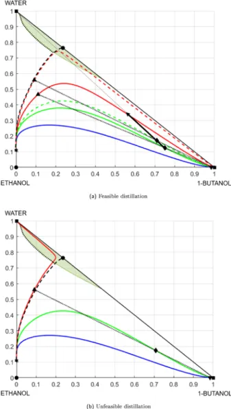
RCMs related to nominal operating conditions are plotted inFigure 7a. The color notation is green for the feed, red for the distillate, and blue for the bottom. The dark green slice shows the region where the liquid phase demixing occurs. In order to account for the eventual presence of two liquid
phases, the option including liquid split calculation in Simulis Thermodynamics has been ticked.
As it can be noticed, under nominal operating conditions, all the distillation column streams belong to the same distillation bundle where n-butanol is the stable node while the water−ethanol azeotrope is the unstable one. In order to be conservative, the temperature used to outline the immiscibility region is the boiling temperature of the unstable node since it corresponds to the lowest value achieved along the residue curve.
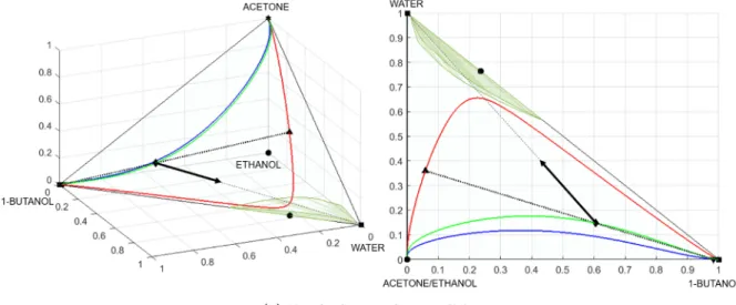
Starting from this operating point, water can be added as usual in order to assess its maximum allowed molar fraction. The addition of water in a ternary diagram, keeping unchanged the quantity of the other compounds, consists of the operating point displacement toward the water vertex as shown by the black arrow inFigure 7a. The distillate and the bottom product compositions can be then calculated based on the specifications and the equilibrium. Since the bottom product composition isfixed by the required butanol purity, by shifting the feed composition, the distillate characteristic point location changes accordingly in order to satisfy the lever rule. The limit feasibility conditions are shown by the dotted lines inFigure 7a and correspond to the feed composition z̅ = [0.709,0.173,0.118]. For a further water content increase, indeed, the distillate stream characteristic point crosses the distillation boundary and falls into the distillation region where the stable node is represented by water instead of n-butanol as shown in Figure 7b.
Beside the effective graphical visualization, there are a few remarks worth doing from a quantitative point of view. The first observation refers to the water−butanol ratio at the feasibility limit; in the case of a binary mixture without decantation, this ratio is approximately 1:6.14, while with the addition of ethanol, the separation feasibility is enhanced until a 1:4.1 ratio. This means that, for this case study, the maximum allowed amount of water is higher if a certain third compound is present.
The second remark states that the increase in this ratio quantitatively depends on the amount of the third species. In particular, from a graphical point of view, a higher ethanol addition reflects in a rotation toward the ethanol vertex [0, 0] of the operating line.
Moreover, as it can be noticed from the plot, the residue curve related to the distillate stream enters the immiscibility region. In this case, its calculation is based on the VLLE and accounts for the liquid phase demixing. The dotted line represents the boundary compositions in case the decanter is exploited to enhance the separation as previously discussed for the binary case study. The same remarks concerning the distillate overcooling keeps being valid for the ternary mixture as well due to the correlation between the immiscibility region and operating temperature.
However, for this case study, the characteristic points are always far from this region; thus, the separation is not concerned by heterogeneous phases in the column.
It is finally worth highlighting that all those results are strictly related to the system thermodynamics and do not take into account operating costs and controllability of the process that could affect the design choice.
6.2. Quaternary System. According to the procedure followed in the ternary case study, the previous boundary composition z̅ = [0.709,0.173,0.118] can be taken as an initial value. Then, an amount of acetone equal to the water molar
fraction can be added and the composition can be re-normalized to z̅ = [0.604,0.148,0.100,0.148].
The so-obtained quaternary mixture can then be represented in a corresponding quaternary diagram. This diagram consists of a 3D pyramid whose vertices correspond
to each pure component; the distillation region in a quaternary diagram is topologically defined by a 3D space and its boundary is a surface, while the mass balance still lies on a line connecting the inlet/outlet characteristic points. Finally, since both the BWE and BWA mixtures show
phase demixing, the immiscibility region is a 3D space included between those two surfaces.
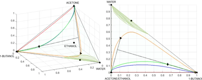
Residue curve mapping can be then performed under nominal operating conditions as shown in Figure 8a where pure ethanol corresponds to the origin of the axes [0,0,0]. All the three curves lie in the same distillation region and an additional water perturbation is possible with respect to the ternary case study. In a quaternary diagram, the addition of a single species keeping unchanged the proportion between the other ones is carried out by shifting the operating point toward the corresponding vertex as usual. Thus, a water increase in the distillation column feed is graphically represented by the black arrow inFigure 8a.
The extreme condition is obtained for a feed composition equal to z̅ = [0.594,0.162,0.099,0.145] as shown inFigure 8b. For a further water content increase in the feed, the residue curve passing through the distillate characteristic point (the red one in thefigure) overcomes the distillation boundary in analogy with the ternary case study, and its stable nodes become pure water instead of pure butanol.Figure 8c shows the unfeasible conditions and the separatrix, which, in this case is a surface, is represented by dashed contour lines.
In analogy with the previous case, it can be concluded that the addition of acetone improved the separation by increasing the maximum allowed water/butanol ratio in the feed from 1:4.1 to 1:3.67.
Even in this case, the result quantitatively depends on the amount of the other species; the maximum allowed water content could indeed increase further for different values of acetone and ethanol content due to the convexity of the separatrix surface.
If the operating points lied in the pure water distillation region, indeed, the addition of acetone and/or ethanol would have reduced the operation flexibility due to the inverse separatrix shape experienced from that side.
The same remarks about convexity apply to the ternary case as well as to mixtures with a higher number of components even though they cannot be graphically represented in a physical space.
Even though calculations have been performed for a given value, the separatrix shape depends on thermodynamics only, and the detailed study of the process feasibility boundaries allows us to assess which maximum allowed perturbation could withstand the distillation system, i.e. its thermodynamic flexibility.
Moreover, it is worth remarking that this analysis refers to one purity constraint and one recovery constraint on the same product (i.e., the separation yield); for different specifications, a dedicated study should be performed.
Finally, it should be highlighted that this study does not account for economic or controllability aspects but it just establishes the physical distillation constraints that cannot be violated independently on the technological solution.
6.3. Systems with More than Four Components. All the examples presented so far are related to mixtures whose
equilibrium diagrams can be visualized in a three-dimensional (or lower) space.
When more than four components are present, the composition domain is a N − 1 D space and the graphical approach cannot be exploited for a more immediate physical understanding. However, from a computational point of view, the way residue curves can be outlined does not change. They are still one-dimensional curves in the composition hyperspace whose coordinates can be obtained by the integration ofeq 1. In order to have a practical example of the analytical approach for the feasibility boundaries’ estimation, let us consider the ABE/W mixture case study if some methanol is present as well in the fermentation broth. According to the usual procedure, given the boundary composition z̅ = [0.594,0.162,0.099,0.145], methanol can be added in the same amount as water and the final composition after n o r m a l i z a t i o n r e s u l t s t o b e z̅ = [0.511,0.139,0.086,0.125,0.139].
Given the separation specifications and the mass balances, bottom and distillate streams compositions are then estimated, the residue curve passing through each one of the three characteristic points can be calculated as usual, and stable and unstable nodes can be easily determined.
Under nominal operating conditions, the residue curves corresponding to the feed and the products have the same stationary points; thus, the separation still results to be feasible even after the addition of methanol. The feed water content can be then perturbed in order to assess the new boundary conditions.
The flexibility assessment results corresponding to the unfeasible condition are presented in Table 1. Although the presence of methanol implies one additional singular point in the composition space, i.e., the acetone−methanol azeotrope, we are able to further enhance the separation. As it can be noticed, the boundary composition for a water perturbation is z̅ = [0.498,0.162,0.083,0.121,0.136], corresponding to a maximum molar water to butanol ratio in the feed of about 1:3.25.
In general, in the feasible region, the unstable node shifts from “acetone” to the “acetone−methanol azeotrope”, while the stable one is still pure butanol. On the contrary, for higher water perturbations, the residue curve passing through the distillate characteristic point ends at the“pure water” node as already experienced in the previous chapters. In any case, the lack of a geometrical representation makes the understanding of the newly generated distillation bundles substantially more difficult.
The additional computational effort due to the presence of a fifth compound is comparable with that related to the previous scale-up.
In conclusion, it is worth remarking that the procedure introduced here above may lead to a feasible domain underestimation when the VLE equilibrium behavior exhibits a nonideality resulting in inflections of the total reflux trajectories as anticipated in the Introduction. Those cases, which are not discussed in this research study, require an Table 1. Analytical Results for Five-Component RCMs
stream zBut zWat zEth zAce zMet stable node unstable node
feed 0.498 0.162 0.083 0.121 0.136 n-butanol acetone−MeOH
bottom 0.972 0.020 0.008 0 0 n-butanol acetone−MeOH
distillate 0.039 0.299 0.156 0.239 0.267 water acetone−MeOH
accurate separatrix hypersurface estimation in order to check if it can be crossed or not in columns operating at total reflux.
7. DISTILLATION TRAINS AND DIVIDING WALL COLUMN
When more than two pure components should be recovered from multicomponent mixtures or if more than two specifications should be satisfied in order to have a profitable separation process, distillation columns can be combined in distillation trains. There exist several distillation train configurations named after the sequencing of the product purification. The most popular are the direct, indirect, and midsplit configurations. The first two consist of several columns in series, and the separation starts from the most volatile compound to the heaviest for the direct and the opposite for the indirect. The midsplit configuration is a parallel configuration where pure compounds are obtained downstream after previous partial splits.
An alternative solution to multicomponent-mixture separa-tion is a dividing wall column, i.e., a single distillasepara-tion column whose central section is divided by one or more walls and with one or more side withdrawals. It represents the arrangement in a single distillation column shell of the Petlyuk column configuration.33 This configuration is equivalent to the distillation train even though only two external duties are present. The reason why it has been studied in depth is that it is the only large-scale process intensification case where both CAPEX and OPEX as well as the required installation space can be drastically reduced.34,35 However, from a thermodynamic point of view, distillation trains and the DWC can be considered equivalent configurations. The Petlyuk arrangement of the DWC, i.e., pre-fractionator and column, and the equivalent indirect configuration are shown inFigure 9for an infinite number of equilibrium stages. The indirect configuration has been selected as a case study since Di Pretoro et al.36,37 already proved it to be particularly convenient for n-butanol recovery
in ABE separation. However, in this paper, the thermody-namic assessment has been extended including both the columns of the distillation train configuration. Furthermore, the following procedure can be scaled up to any number of columns, i.e., any number of walls and side streams in a DWC. The residue curve interpretation does not considerably change. It still represents the column concentration profile for an infinite number of trays at an infinite reflux ratio. The main consequences of this theoretical consideration is that the distillation feasibility condition still applies: in order to belong to the same distillation column profile, the residue curves passing through the characteristic point of every side stream should belong to the same distillation region, i.e., it should have the same stable and unstable nodes. Thus, the main change with respect to the single column case study is that all the streams entering or exiting the distillation train (or the DWC) should be included in the analysis.
As already anticipated in Section 4, the additional specifications to be included will refer to the acetone purity and recovery ratio; this means that the side stream will contain the remaining components, i.e., mainly water and ethanol. While the specification related to a product purity directly provides its coordinate in the diagram, the recovery ratio constraint requires a reinterpretation.
By performing the overall mass balance on the entire system, the following equation can be easily obtained:
= + + F D S B (4) that is: = D + + F S F B F 1 (5)
On the other hand the partial mass balance states as:
· ̅ = · ̅ + · ̅ + · ̅
F z D xD S xS B xB (6)
dividing everything by F the equation of a plane is achieved:
Figure 10.Distillation RCM for distillation train and DWC.
̅ = · ̅ + · ̅ + · ̅ z D F x S F x B F x D S B (7)
This means that, for given product compositions (x̅D and
x̅B) and recovery ratios (directly related to D F and
B
F), the side stream molar fractions andflow rate can be assessed and the corresponding characteristic point lies on the same plane as the other three.
In conclusion, the mass balance in a quaternary diagram is translated into a coplanarity condition and the recovery ratios establish the relative position of the side stream characteristic point with respect to the distillate and the bottom ones.
T h e r e f o r e , a g i v e n i n l e t c o n c e n t r a t i o n z̅ = [0.660,0.120,0.100,0.120] similar to the ones in the previous chapter is assumed. Residue curves under nominal operating conditions are calculated as usual for the four streams and plotted in Figure 10a. The orange curve refers to the side stream, while the color notation for the other curves is unchanged. Water content, which is the most critical parameter, can be then perturbed as usual until feasibility limits are achieved for z̅ = [0.641,0.146,0.097,0.116] as plotted in Figure 10b. For a further increase in the water molar fraction, the residue curve related to the side stream crosses indeed the distillation boundary and does not attain the pure butanol vertex but the pure water one instead.
Even though the case study is different from the one in the previous chapter since a second compound, i.e., acetone, is recovered as well, the feasibility boundary values can be commented in analogy to the single distillation column.
First of all, it is worth noticing that the separatrix surface is the same as the single column case study since it is a function of the system thermodynamics, i.e., of the components only.
While, for the single column, the distillate stream is the one crossing the distillation boundary, in the case of indirect distillation train and the DWC, the second column bottom stream and the side stream are those who cause the process unfeasibility.
For this case study, the limit water to butanol ratio is 1:4.4 resulting in a substantial decrease with respect to the previous cases where acetone was not purified. Due to the acetone recovery, a consistent amount of ethanol is indeed withdrawn in the distillate stream. This causes the side withdrawal to be richer in water both because acetone is not present anymore and because it carries with it part of the ethanol causing a faster shifting of the side stream operating point toward the pure water vertex.
As anticipated, this procedure has no upper limits concerning the number of species in the feed and the number of column/walls, but at least three components are required in order to have a useful employment of distillation trains or DWC.
8. CONCLUSIONS
Residue curve mapping has been deeply explored in this analysis. Three main outcomes can be identified from this study and are worth commenting on.
The first one is the definition of a thorough procedure to assess thermodynamicflexibility of distillation processes when the product recovery ratio is used as a separation specification. This parameter indeed can be directly correlated to the separation productivity that is the main income item in process design. Depending on the number of components, the recovery ratio fixes the relative position of the distillation
column streams over the N− 2 dimensional space constrained by the mass balances.
The second useful tool described in this paper is the thermodynamic feasibility assessment and definition of flexibility boundaries in the case of distillation trains and integrated distillation systems such as the DWC as well as its graphical representation. Since, at infinite reflux and number of equilibrium stages they are equivalent configurations, there is no difference concerning the thermodynamic feasibility limits. However, when dealing with costs and control, they are likely to show considerably different behaviors.
Finally, according to the shape of the N-dimensional separatrix boundary, RCM graphical representations allow us to predict the effect of the presence of a further component in the feed stream from a flexibility point of view. The convexity/concavity of the separatrix would result respectively in a positive/negative impact on the separation effectiveness under uncertainty.
In conclusion, this study provides a useful graphical and numerical tool to the decision maker in order to evaluate the potentialities and the limitations of the most common distillation processes applied to a given multicomponent mixture. Even though the presented results are case-specific, the proposed procedure has a general validity and can be performed with any mixture and any of the most-used flexibility indexes.
Residue curve mapping has proved indeed to be an effective methodology worth exploiting even when uncertainty should be taken into account that is particularly the case with bio-based processes.
■
AUTHOR INFORMATIONCorresponding Author
Ludovic Montastruc − Laboratoire de Génie Chimique, Université de Toulouse, CNRS/INP/UPS, Toulouse 31100, France; Email:[email protected]
Authors
Alessandro Di Pretoro − Laboratoire de Génie Chimique, Université de Toulouse, CNRS/INP/UPS, Toulouse 31100, France; Dipartimento di Chimica, Materiali e Ingegneria Chimica ≪Giulio Natta≫, Politecnico di Milano, Milano 20133, Italy;
Flavio Manenti − Dipartimento di Chimica, Materiali e Ingegneria Chimica≪Giulio Natta≫, Politecnico di Milano, Milano 20133, Italy
Xavier Joulia − Laboratoire de Génie Chimique, Université de Toulouse, CNRS/INP/UPS, Toulouse 31100, France Complete contact information is available at:
Notes
The authors declare no competing financial interest.
■
ABBREVIATIONSABE/W acetone−butanol−ethanol/water B bottomflow rate (mol/s)
Cijn excess Gibbs energy coefficients (J/(mol·Kn))
CAPEX capital expenses ($) D distillateflow rate (mol/s) DWC dividing wall column F feedflow rate (mol/s)
Ki equilibrium constant (1) NRTL nonrandom two liquids OPEX operating expenses ($/year) P pressure (atm)
R gas constant (J(mol·K)) RCMs residue curve maps
S side streamflow rate (mol/s) T temperature (°C)
VLLE vapor−liquid−liquid equilibrium
xik kth-stage liquid-phase molar fraction of the ith
species (1)
xiaq/org Aqueous/organic phase molar fraction of the ith
species (1)
x̅ liquid-phase composition vector (1)
yi vapor-phase molar fraction of the ith species (1) y̅ vapor-phase composition vector (1)
zi molar fraction of the ith species in the feed (1) z̅ feed composition vector (1)
αi,j nonrandomness parameter (1)
γi activity coefficient (1)
ξ dimensionless time (1)
τi,j NRTL dimensionless interaction parameter (1)
■
REFERENCES(1) Di Pretoro, A.; Montastruc, L.; Manenti, F.; Joulia, X. Flexibility analysis of a distillation column: Indexes comparison and economic assessment. Comput. Chem. Eng. 2019, 124, 93−108.
(2) Hoch, P. M.; Eliceche, A. M.; Grossmann, I. E. Evaluation of Design Flexibility in Distillation Columns Using Rigorous Models. Comput. Chem. Eng. 1995, 19, 669−674.
(3) Giuliano, A.; Poletto, M.; Barletta, D. Process optimization of a multi-product biorefinery: The effect of biomass seasonality. Chem. Eng. Res. Des. 2016, 107, 236−252.
(4) Yue, D.; You, F.; Snyder, S. W. Biomass-to-bioenergy and biofuel supply chain optimization: Overview, key issues and challenges. Comput. Chem. Eng. 2014, 66, 36−56.
(5) Ostwald, W. Dampfdrucke ternarer Gemische. Ges. Wiss. 1900, 25, 413−453. (Germ.)
(6) Schreinemakers, F. A. H. Dampfdrucke ternarer Gemische. Z. Phys. Chem. 1901, 36, 413−449. (Germ.)
(7) Gurikov, Y. V. Some Questions Concerning the Structure of Two-Phase Liquid− Vapor Equilibrium Diagrams of Ternary Homogeneous Solutions. Zh. Fiz. Khim. 1958, 32, 1980−1996. (Rus.)
(8) Zharov, V. T. Free Evaporation of Homogeneous Multi-component Solutions. Russ. J. Phys. Chem. 1967, 41, 1539−1555. (Rus.)
(9) Zharov, V. T. Free Evaporation of Homogeneous Multi-component. Solutions. 2. 4-Component Systems. Russ. J. Phys. Chem. 1967, 42, 1539. (Rus.)
(10) Zharov, V. T. Free Evaporation of Homogeneous Multi-component Solutions. 3. Behavior of Distillation Lines Near Singular Points. Russ. J. Phys. Chem. 1968, 42, 195−211. (Rus.)
(11) Serafimov, L. A. The Azeotropic Rule and the Classification of Multicomponent Mixtures. 4. N-Component Mixtures. Russ. J. Phys. Chem. 1969, 43, 981−983. (Rus.)
(12) Zharov, V. T., Serafimov, L. A. Physico-Chemical Foundations of Bath Open Distillation and Distillation; Khimiya: Leningrad, 1975. (Rus.)
(13) Petlyuk, F. B.; Danilov, R. Y. Theory of Distillation Trajectory Bundles and its Application to the Optimal Design of Separation Units: Distillation Trajectory Bundles at Finite Reflux. Chem. Eng. Res. Des. 2001, 79, 733−746.
(14) Petlyuk, F.B. Distillation Theory and its Application to Optimal Design of Separation Units; Cambridge University Press: 2004,
DOI: 10.1017/CBO9780511547102.
(15) Laroche, L.; Bekiaris, N.; Andersen, H. W.; Morari, M. Homogeneous azeotropic distillation: separability and flowsheet synthesis. Ind. Eng. Chem. Res. 1992, 31, 2190−2209.
(16) Thormann, K. Destillieren und Rektifizieren; Springer-Verlag: (Germ.), 2013.
(17) Kiva, V. N.; Hilmen, E. K.; Skogestad, S. Azeotropic phase equilibrium diagrams: a survey. Chem. Eng. Sci. 2003, 58, 1903− 1953.
(18) Wahnschafft, O. M.; Koehler, J. W.; Blass, E.; Westerberg, A. W. The product composition regions of single-feed azeotropic distillation columns. Ind. Eng. Chem. Res. 1992, 31, 2345−2362.
(19) Saboo, A. K.; Morari, M.; Woodcock, D. C. Design of resilient processing plantsVIII. A resilience index for heat exchanger networks. Chem. Eng. Sci. 1985, 40, 1553−1565.
(20) IEA Bioenergy; 2018 retrieved at https://www.ieabioenergy. com/wp-content/uploads/2019/04/IEA-Bioenergy-Annual-Report-2018.pdf.
(21) García, V.; Päkkilä, J.; Ojamo, H.; Muurinen, E.; Keiski, R. L. Challenges in biobutanol production: How to improve the efficiency? Renewable Sustainable Energy Rev. 2011, 15, 964−980.
(22) Ezeji, T. C.; Qureshi, N.; Blaschek, H. P. Bioproduction of butanol from biomass: from genes to bioreactors. Curr. Opin. Biotechnol. 2007, 18, 220−227.
(23) Xue, C.; Zhao, J.-B.; Chen, L.-J.; Bai, F.-W.; Yang, S.-T.; Sun, J.-X. Integrated butanol recovery for an advanced biofuel: current state and prospects. Appl. Microbiol. Biotechnol. 2014, 98, 3463− 3474.
(24) Errico, M.; Sanchez-Ramirez, E.; Quiroz-Ramìrez, J. J.; Rong, B.-G.; Segovia-Hernandez, J. G. Multiobjective Optimal Acetone− Butanol− Ethanol Separation Systems Using Liquid− Liquid Extraction-Assisted Divided Wall Columns. Ind. Eng. Chem. Res. 2017, 56, 11575−11583.
(25) Renon, H.; Prausnitz, J. M. Local Compositions in Thermodynamic Excess Functions for Liquid Mixtures. AIChE J. 1968, 14, 135−144.
(26) Kiss, A. A. Novel applications of dividing-wall column technology to biofuel production processes. J. Chem. Technol. Biotechnol. 2013, 88, 1387.
(27) Okoli, C. O.; Adams, T. A., II Design of dividing wall columns for butanol recovery in a thermochemical biomass to butanol process. Chem. Eng. Process. 2015, 95, 302.
(28) Le, Q.-K.; Halvorsen, I. J.; Pajalic, O.; Skogestad, S. Dividing wall columns for heterogeneous azeotropic distillation. Chem. Eng. Res. Des. 2015, 99, 111−119.
(29) Dortmund Data Bank;www.ddbst.de.
(30) Luyben, W. L. Control of the Heterogeneous Azeotropic n-Butanol/Water Distillation System. Energy Fuels 2008, 22, 4249− 4258.
(31) Stockhardt, J. S.; Hull, C. M. Vapor-Liquid Equilibria and Boiling-Point Composition Relations for Systems n-Butanol− Water and Isobutanol− Water1,2. Ind. Eng. Chem. 1931, 23, 1438−1440.
(32) Orr, V.; Coates, J. Versatile Vapor-Liquid Equilibrium Still. Ind. Eng. Chem. 1960, 52, 27−30.
(33) Petlyuk, F. B. Thermodynamically Optimal Method for Separating Multicomponent Mixtures. Int. Chem. Eng. 1965, 5, 555−561.
(34) Glinos, K.; Malone, M. F. Optimality Regions for Complex Column Alternatives in Distillation Systems. Chem. Eng. Res. Des. 1988, 66, 229−240.
(35) Schultz, M. A.; Stewart, D. G.; Harris, J. M.; Rosenblum, S. P.; Shakur, M. S.; O’Brien, D. E. Reduce costs with dividing-wall columns. Chem. Eng. Prog. 2002, 98, 64−71.
(36) Di Pretoro, A.; Montastruc, L.; Manenti, F.; Joulia, X. Flexibility Assessment of a Distillation Train: Nominal vs Perturbated Conditions Optimal Design. Comput.-Aided Chem. Eng. 2019, 46, 667−672.
(37) Di Pretoro, A.; Montastruc, L.; Manenti, F.; Joulia, X. Flexibility assessment of a biorefinery distillation train: Optimal