Open Archive TOULOUSE Archive Ouverte (OATAO)
OATAO is an open access repository that collects the work of Toulouse researchers and
makes it freely available over the web where possible.
This is an author-deposited version published in :
http://oatao.univ-toulouse.fr/
Eprints ID : 16471
To link to this article : DOI : 10.1016/j.ces.2016.10.024
URL :
http://dx.doi.org/10.1016/j.ces.2016.10.024
To cite this version : Bacchin, Patrice An energy map model for
colloid transport. (2017) Chemical Engineering Science, 158. pp.
208-215. ISSN 0009-2509
Any correspondence concerning this service should be sent to the repository
administrator:
[email protected]
An energy map model for colloid transport
Patrice Bacchin
Laboratoire de Génie Chimique, Université de Toulouse, CNRS, INPT, UPS, Toulouse, France
A B S T R A C T
When dispersed colloids areflowing, they experience interactions with the fluid (friction) and with other colloids (surface interactions). These phenomena are usually taken into account through a Suspension Balance Model (SBM) that couples mass and momentum balances. However, in many applications, the dispersed particlesflow close to an interface or inside a porous media. The flow in such a confined environment leads to significant particle-wall interactions. This paper puts forward an energy map model that accounts for these particle-wall interactions. A way to implement the energy map in the SBM is to introduce an interfacial pressure concept. The new possibilities opened up by the energy map that account for interfacial interaction in the SBM are analysed. A transient 1D case study for the transfer of colloids through a pore illustrates the potentialities of the Suspension Balance Model integrating an Energy Map (SBM-EM). The model enables the description of the transmission of the colloids through the energy map representing the membrane (mass balance) and the consequences in terms of an out-of-equilibrium counter pressure (momentum balance). The counter osmotic pressure is then explained by the interfacial interaction between the colloids and the interface; these interfacial interactions that prevents the colloids from leaving the bulk volume generate forces that are transmitted to the fluid (via the drag force), thus inducing osmosis. The energy map model can enable the incorporation of the physical and chemical heterogeneities of the interacting surfaces. It might be of interest to explore the transfer of colloids along or inside real surfaces (being a mosaic of nano- or micro-scale domaines with specific interactions).
1. Introduction
The transport of colloids cannot be described only by classical diffusive and convective mass transport terms. The main reasons are the existence of both surface interactions between the colloids (or between a colloid and its surrounding interface) and hydrodynamic interactions between the particle and thefluid (interactions with the shear rate). These interactions that occurs at a nano- or micro-scale are deeply modifying the way in which colloids are diffusing and/or being advected. For example, processes such as ultrafiltration, nanofiltration or reverse osmosis, which are classically used to purify, eliminate and concentrate colloids or nanoparticles, strongly depend on these inter-facial phenomena. The level of fouling, its kinetics or even the way colloids build up (porosity, hydraulic resistance or accumulation reversibility) are driven by colloidal properties (Bacchin et al., 2011). Such an impact of surface interactions is also crucial during the transport of drug and carriers in the crowd environment of cells ( Al-Obaidi and Florence, 2015); the nano-scale interactions playing a significant role on the hindered diffusion or advection towards cellular goals.
It is therefore necessary to establish experimental and theoretical
connections between colloidal properties at a local (micro) scale and the efficiency of the mass and momentum transport phenomena; this knowledge is compulsory for the control of numerous processes that deal with concentrated colloids and/or colloids in confined situations. In a sheared flow, the colloids are submitted to hydrodynamic interactions (due to thefluid velocity-drag force and to the velocity gradient-shear induced diffusion or lateral migration). Additionally, in a concentratedflow, colloids experience multi-body surface interaction (i.e. DLVO forces, etc.). In theseflows, it is crucial to account for the momentum coupling or exchange between thefluid and the particle phase. These interactions (and their coupling) can be taken into account by the Lagrangian approach (like the Force Coupling Method or the Monte Carlo procedure) or by the Eulerian approaches (twofluid model, mixture models, suspension balance model). Multiple inter-particle DLVO interactions have been implemented in the Force Coupling Method in order to depict the collective effect induced by thefiltration through a pore (Agbangla et al., 2014). However, this method, based on the tracking of individual particles (around 1 µm), remains impossible to apply for describing the process scale (around 1 m). For this reason, the Eulerian approach that considers the variation of spatial averaged variables, is more adapted for the
http://dx.doi.org/10.1016/j.ces.2016.10.024
description of the transport of concentrated colloidal dispersion. The different hydrodynamic and colloidal forces can be accounted for with two coupled momentum balances for both the particle phase and the fluid phase (called for this reason the two fluid model (Noetinger, 1989)). These momentum balances are coupled by considering mo-mentum exchanges. According to this formulation, the equation can be written for the whole mixture (particles andfluid). It is then called the suspension balance model (Nott and Brady, 1994) or the mixture model (Jackson, 2000, 1997). Both the momentum exchange between the particle and the fluid phases and the slip velocity between the particles and thefluid have to be introduced as closure relationships in order to fully describe the problem. This last Eulerian approach will be introduced in the background section of this paper.
However, the picture is even more complex when the flow of particles takes place in confined conditions, where interactions with the walls are occurring. Furthermore, real surfaces are often chemically heterogeneous on a micro- or a nano-scale (like a biological membrane composed of lipid bilayers with inclusions) and can present local morphological heterogeneity (for example asperities) that can induce different local interaction energies when an object approaches the surface. To account for this complexity, the particle-wall interactions can be accounted for through an energy map. Several authors have defined interactions maps to characterise the approach of colloids near a surface. Interaction maps allows for example, the effect of the roughness, through DLVO calculations (Hoek et al., 2003), to be described. These maps have been used to determine the local equili-brium position that is due to both lateral and normal components of the DLVO force (Kemps and Bhattacharjee, 2005). Comparing the hydrodynamic forces with a DLVO energy map can then help to have a better evaluation of the interactions between colloids and heteroge-neous surfaces (Shen et al., 2012). However, this energy map should be integrated in a full transport model in order to account for the coupling with diffusion, advection and hydrodynamic or colloidal interactions.
The aim of this paper is to propose a model that describes the transport of colloids in (or close to) porous media and thus to integrate the effect of both particle/particle and particle/wall interactions. The approach taken will be to implement an energy map (for an interacting surface) in a Suspension Balance Model.
2. Theoretical background
The Suspension Balance Model SBM (Nott and Brady, 1994) was initially established to describe the non-Brownian migration of parti-cles in suspension. The shear-induced migration was depicted by considering the effect of particles in the fluid phase through a particle-phase stress previously introduced by Batchelor (1970). This work and further implementations (Morris and Boulay, 1999) allow to relate the rheology of the suspension to the migration flux (mass transfer) of particles. They demonstrated that the SBM approach was encompassing the diffusive flux model (previously introduced by
Leighton and Acrivos (1987)), based on an empirical consideration that massflux is proportional to gradients in particle concentration and shear rate. More recently,Lhuillier (2009)discussed the discrepancies between the two-fluid approach and the SBM and proposed that the force exchange on the particle phase was the sum of the interphase drag forces,Fdrag(arising from the difference in velocity between the
particles and thefluid phases) and a stress-induced force,Σp(arising
from the gradient in the field of velocity). A review of the mixture models for shear-induced migration in flowing, viscous and concen-trated particle suspensions have highlighted the possibility of describ-ing the non-equilibrium osmotic pressure and shear-induced diffusion coefficients in the same model formulation (Vollebregt et al., 2010). All these recent developments have been integrated in a revisited form of the Suspension Balance Model (Nott et al., 2011) that will be the starting point of the analysis done in the paper.
2.1. The suspension balance model (SBM)
The SBM is based on solving field equations written from the volumic averaging of the governing equations (local momentum and mass balances) on the two phases. Thesefield equations resulting from momentum and mass balances, are written below for thefluid phase, the dispersed phase and the mixture (the balance for the mixture being the sum of the two phases):
Momentum balance
For the dispersed phase
Σ
ϕρ g nFp→+ ⎯→ +∇⋅ =0⎯ drag p (1)
For thefluid
e Σ
ϕ ρ g nF ϕ p η
(1 − ) ⎯f→− ⎯→ −∇(1 − ) +2 ∇⋅< > + ∇⋅ =0drag f f (2)
For the mixture
e Σ Σ
ρ gm→−∇(1 − ) +2 ∇⋅< > + ∇⋅ +∇⋅ =0⎯ ϕ p ηf p f (3) Mass balance
For the dispersed phase
ϕ t ϕu
∂
∂ =−∇⋅( ⎯→ )p (4)
For thefluid
ϕ
t ϕ u
∂(1− )
∂ =−∇⋅((1 − ) ⎯→ )f (5)
For the mixture
u
0 = ∇⋅⎯→m (6)
The revisited form (Nott et al., 2011) considers a momentum exchange between the dispersed and thefluid phase via a drag force,
nF⎯→drag, and a contribution to the mixture momentum through the
divergence of a particle stress,∇⋅Σp, and through the divergence of a
fluid stress,∇⋅Σf. In the momentum balance, the other terms are the
effect of the gravity of each phases, the fluid pressure gradient and the viscosity of thefluid phase (whereeis the strain rate tensor linked to the shear rate∇ /2 = ̇/2uf γ for an uniaxialflow). The mass balances
introduces the advectiveflux of the particle,up, thefluid velocity,uf,
and the mixture velocity um coming from volume averaging,
ϕu +(1 − )up ϕ f.
2.2. A set of closure relationships for colloids
Closure relationships are necessary to close the problem and to be able to determine thefluid properties (the velocity and the volume fraction) from the previous set of equations (Eqs. (1)–(6)). A first closure relationship expresses the drag force as a function of the slip velocity between the particle phase,up, and the mixture phase,um:
nF ϕ V u u m ϕ ⎯→ =− ⎯→ − ⎯→⎯ ( ) drag p p m (7) wherem ϕ( )is the mobility of the particles accounting for the effect of the volume fraction, i.e.K ϕ( )/6πμawhereK ϕ( )is the hindered settling coefficient.
The writing of the stressesΣpandΣf is more controversial and a
different set of closure relationships have been proposed (as reviewed inVollebregt et al. (2010)). As underlined byLhuillier (2009), some of these sets of closure presents some inconsistencies. Clausen (2013)
proposes a more consistent formulation: this set of modified closure relationship will be the starting point of the one proposed in this paper. For low Péclet numbers, the particle-phase stress,Σp, can be written
by considering only the normal stress (NS) contribution (Clausen, 2013). Furthermore, a reasonable premise for colloidal particles at moderate shear rates is to consider the stress as isotropic (Hallez et al.,
2016)) and equal to the particle pressure:
Σp=ΣpNS= −Πcc( , ˙) = −(ϕ γ I Πcc th( ) +ϕ Πcc mc( , ˙))ϕ γ I (8)
where Πcc( , ̇)ϕ γ is the generalized concept of particle pressure
(Deboeuf et al., 2009). Particle pressure includes different contribu-tions that can be shared accordingly:
•
The thermodynamic osmotic pressure,Πcc th( ),ϕ that also representsthe equation of state for colloids accounting for the entropic contribution Πcc ent( )ϕ and the multi-body interactions (van der
Waals, electrostatic, etc.) Πcc mbi( )ϕ. The gradient in the osmotic
pressure is directly linked to the chemical potential gradient and therefore to a thermodynamic force. This contribution is a reversible thermodynamic property (elastic contribution) when the dispersive forces (entropic or electrostatic) overcome the attraction i.e. if
>0.
dΠ dϕ
cc th If this last derivative is negative (for example when high
concentration lead colloids to interact at shorter distances with attractive interactions), a spinodal decomposition occurs. Colloids are no longer spontaneously thermodynamically dispersed: colloids can interact with mechanical interactions and the particle pressure is no longer osmotic (when osmotic is defined as an idealized, spontaneous reversible and non-dissipative process, constituted of a continuous sequence of equilibrium states).
•
The mechanical particle pressure,Πcc mc( , ̇)ϕ γ is the contribution ofthe particle pressure due to mechanical contact between colloids (inelastic collisions, friction) or between colloids and the fluid presenting a dissipative irreversible character (viscous contribu-tion). This contribution can be composed of the shear-induced normal stress term of the particle-phase stress Πcc shr( , ̇)ϕ γ, when
the concentrated particles are sheared, and the compressive yield stress (Buscall and White, 1987) when the particles are in contact,
Πcc cys( )ϕ.
The fluid stress acting on the fluid momentum balance can be defined as the contribution of the particle phase to the viscosity,η ϕp( ),
and of the thermodynamic osmotic pressure,Πth( )ϕ:
Σf= 2η η ϕf p( ) < > +e Πcc th( )ϕI (9)
The particle contribution to the viscosity combines with2 ∇.< >ηf e to
represent the shear viscosity of the mixture: ηm( )= (1+ ( )ϕ ηf η ϕp . The
thermodynamic osmotic pressure is here accounted as an exchange between the particle and the fluid phases, as proposed byLhuillier (2011)for the thermodynamic forces within the interphase force.
The addition of Eqs.(8) and (9)(also defined by Batchelor's,Σs, the
solid-phase stress) defines the total stress for the mixture (Eq. (3)), thus accounting for a viscous term and a particle pressure term:
Σp+Σf= 2η η ϕf p( ) < > −e Πcc mc( , ˙)ϕ γ I (10)
This writing is consistent with the most commonly form (Miller et al., 2009; Morris and Boulay, 1999) for non-Brownian suspensions, accounting for a non-Brownian particle pressure contribution when assuming no significant normal-stress difference.
2.3. The set of Eulerian equations to solve
Combining the field equations (Section 2.1) and the modified rheological model enables o the set of the Eulerian equation to solve to be defined.
Momentum balance
For the dispersed phase
I I
ϕρ gp→ + ⎯→ − ∇.⎯ nFdrag Πcc th − ∇.Πcc mc = 0 (11)
For thefluid
e I
ϕ ρ g nF ϕ p η Π
(1 − ) ⎯f→ − ⎯→ − ∇(1 − ) + 2∇.drag m< > + ∇. cc th = 0
(12) For the mixture
e I
ρ gm→−∇(1 − ) +2 ∇.⎯ ϕ p ηm< > − ∇.Πccmc =0 (13) Mass balance
For the dispersed phase
ϕ
t ϕu
∂
∂ =−∇. ( ⎯→ )p (14)
For thefluid
ϕ
t ϕ u
∂(1− )
∂ =−∇. ((1 − ) ⎯→ )f (15)
For the mixture
u
0 = ∇. ⎯→m (16)
The momentum balance for the particle phase (Eq.(11)) permit the drag force to be expressed. The drag force being linked to the slipping velocity (Eq. (7)), it is possible to express the particle velocity as follows: u u m ϕ V ρg Π ϕ ⎯ → =⎯→ + ( ) ( ⎯→−∇ )p m p cc (17) The particle velocity can be implemented in the mass balance for the dispersed phase (Eq.(14)) leading to Eq.(20). This equation has to be solved together with the Eqs. (18) and (19) (the mixture mass balance and the mixture momentum balance respectively) to have the full set of the 3 SBM equations:
u ∇.⎯→ =0m (18) e I ρ gm→ − ∇(1 − ) + 2∇⋅ ( ) < > − ∇⎯ ϕ p ηm ϕ Πcc mc = 0 (19) ϕ t u ϕ m ϕ V ϕρg Π ∂ ∂ =−∇⋅(⎯→m ) − ∇⋅( ( ) (p →−∇ ))⎯ cc (20)
The solving of these 3 equations then enables the identification of the mixture velocity,um, thefluid pressurep, and the volume fraction of colloids,ϕ. The other variable can easily be determined from this 3 variables; for example the particle velocity can be determined from Eq.
(17).
2.4. Physical consistencies of the set of equations
It has to be noted that the gradient of the complete particle pressure,∇Πcc (combining thermodynamic and mechanic
contribu-tions) acts in the mass transport equation (Eq.(20)) as proposed in the classical diffusive flux model (Deboeuf et al., 2009; Leighton and Acrivos, 1987). However, the momentum, due to the gradient of the thermodynamic contribution of the solid pressure, is released in the fluid (Eq.(12)). Consequently, only the gradient of the mechanical part of the particle pressure,∇Πmc, plays a role on the momentum balance of
the mixture (Eq.(13)). This differentiation of the solid pressure action emphasizes the dual behavior of colloids that are both exchanging “thermodynamical” energy with the fluid, due to the Brownian motion (collisions with the liquid molecules) and dissipate “mechanical” energy in the mixture (collisions and friction with the particles). Such a way to write models enables the description of the equilibrium between the static pressure and the osmotic pressure (Eq.(12)leads to
I
ϕ p Π
∇(1 − ) = ∇. cc th ) when the drag force is zero (at equilibrium).
Furthermore, for non-equilibrium conditions, the Eq.(11) describes the equivalence between drag force and the gradient in osmotic pressure as already discussed by Wijmans et al. (1985) and
Elimelech and Bhattacharjee (1998)for polarization concentration. At the end, as schematized inFig. 1, in this rheological model for the phase stresses, the presence of colloidal particles under a given load
(under a shear rate and under a concentration gradient) contributes to the modification of the momentum exchanges with:
•
a dissipative contribution in thefluid phase,2∇.η η ϕf p( ) < >e due tothe particle phase. Such a term contributes to the mixture effective viscosity in the Stokes equation.
•
a storage contribution in the solid phase through the gradient in particle pressure, −∇.Πcc( , ̇)ϕ γ I. The particle pressure hereac-counts for the storage of the energy in concentrated or high-sheared zone. The thermodynamic contribution to this energy∇.Πcc th( )ϕI
can be later released in thefluid phase. The storage is then an elastic contribution (occurring only when a force is applied i.e. non-permanently). The similarity between osmotic pressure and storage modulus of viscoelastic dispersion has been experimentally evi-denced (Mason et al., 1997). The other part of the energy storage, due to mechanical interaction−∇.Πcc mc( , ˙)ϕ γ I, can be released in
the mixture, where it will be dissipated.
A key feature of this proposed set of modified closure relationships for colloids is the differentiation between the thermodynamic and the mechanic parts of the particle pressure that are acting on thefluid and mixture momentum balances, respectively.
3. Implementation of an energy map in SBM: the SBM-EM model
When colloidsflow close to an interface or inside a porous material, each particle experiences an additional force that can result in a force toward the bulk if the interactions are repulsive or toward the surface if the interactions are attractive. It is possible to access this force by performing the derivative of the interaction energy. The colloid/inter-face potential interaction energy (a free energy),Vic, can be calculated
for each point of thefluid where the particle can flow, then, constituting an energy landscape: the energy map,V( , , )ix y z. This energy map can
also be associated to a pressure, consideringV=V Πi p iwhereΠ ( , , )i x y z is
the interfacial pressure (that can also be the mapped parameter). The associated force per unit of particle volume is given by the interfacial pressure gradient∇Πi. The additional force per unit of volume offluid
is then the product of the volume fraction, multiplied by the gradient of the interfacial pressure:
ϕ Π
− ∇ i (21)
This term is implemented in the dispersed phase momentum balance (Eq. (11)). The term − ∇Π (x, y, z)ϕ i can also be written
Π x y z ϕ
−∇ ic( , , , )whereΠic is the contribution of the interface to the
colloid bulk pressure,Πcc( )ϕ.
The new set of equations is given inSupplementary information (S3). When the SBM equation is combined together with the closure relationship (as previously discussed in Section 2.3), a set of three equations (later called SBM-EM for Suspension Balance Model with Energy Mapping) has to be solved.
Conservation of the velocity of the mixture:
u ∇. ⎯→ =0m (22) Momentum balance e ρ gm→ − ∇(1 − ) + 2∇. ( ) < > − ∇⎯ ϕ p ηm ϕ Πcc mc( ) − ∇ ( , , ) = 0ϕ ϕ Π x y zi (23) Mass balance ϕ t u ϕ m ϕ V ϕρg Π ϕ ϕ Π x y z ∂ ∂ =−∇. (⎯ → ) − ∇. ( ) ( →−∇ ( )− ∇ ( , , ))⎯ m p cc i (24) It has to be noted, that even if the physical context is different, this set of equations can show some similarities with the ones used by
Jacazio et al. (1972). These describe electro-osmosis where the Nernst Planck equation is combined with the Navier Stokes equation that includes an electrokinetics term for the exclusion of ions by the stationary phase.
4. The energy map: an ingredient to understand complex mechanisms
In a general way, the interfacial energy introduced in the energy map,V Π ( , , )p ix y z, can be defined as the energy needed to bring the
dispersed phase close to the interface. It has to be noted that this interfacial pressure presents some similarities with a disjoining pres-sure (Derjaguin and Churaev, 1974). This energy can take different forms and thus describe different mechanisms. In the most conven-tional way, this interaction energy can represent the potential interac-tion energy between the particle and the interface (for example through particle/wall surface interactions: electrostatic interaction, van der Waals, polymer brush, etc.). However, this energy can also reflect the potential energy that an object must acquire in order to be transported in the map. For example, this energy can represent the stretching energy that is required to deform a plasmid DNA and, then, to enable its penetration inside a channel (Li et al., 2015). This energy can also represent the energy needed for a molecule to be solubilized in a material (as in the diffusion/solubilization model in reverse osmosis). This colloid/interface energy can then help to take into account various types of interaction in a global way: the interaction of the colloid with the interface but also the internal interaction within the colloid (change in configuration or phase change) needed to be transferred. (Fig. 2).
The consequences of the introduction of the energy map in Eqs.
(23) and (24)canfirst be investigated by analysing the contribution of each term of the SBM-EM model and secondly, by considering the mechanisms that can be described when coupling two of these terms: – classically, the coupling of the convective termumϕand the diffusive massfluxm(ϕ)V ∇p Πcc describes the polarization layer mechanism
that can develop in a boundary layer. The effect of the multibody interaction and of the shear induced diffusion can be accounted through theΠcc thand theΠcc shcontributions respectively.
– the coupling of the diffusive mass flux∇Πcc with the interfacial
pressureϕ Π∇ idescribes the distribution of the concentration with
the interfacial pressure: an exclusion if the interfacial pressure is positive (repulsion) or an accumulation if the interfacial pressure is negative (attraction). When considering the distribution of the colloids between two phases having a difference of interfacial pressureΠi, a partition coefficient, K, can be defined as the ratio
between the concentration in the phase (where it existsΠi) and the
concentration in the bulk phase (whereΠi=0). With the limits of an
Fig. 1. Schematic view of the SBM modified rheological model for colloidal dispersion. The load in the dispersion (exerted through the shear rate or the density) acts both on the fluid and the particle phases. These phases exchange momentum through the interphase drag force. The different phases can dissipate energy through viscosities (one part coming through the viscosity of thefluid and another from the viscosity induced by the particles – a function of their density,ϕ, and the way particles are sheared,γ̇). The different phases can also contribute in storing the mechanical energy (one part being stored in the fluid-through thefluid pressure, p- and one part being stored in the particle phase in high density,ϕ, or/and in high sheared zone,γ̇-through the particle pressure).
ideal non-interacting dispersion (if the osmotic pressure follows the Van’t Hoff law), this equilibrium leads to a Boltzmann distribution:
Π ϕ Π K e −∇ cc− ∇ =0 ⇐⇒ =i ideal Π V kT − i p (25) – the coupling of the convectionumϕand the interfacial pressure term
m(ϕ)V ∇p Πccrepresents the balance between the hydrodynamic drag
force and the particle-wall force
– in the momentum balance, the coupling between the hydrostatic pressure,−∇(1 − )ϕ pand the interfacial pressure,− ∇ϕ Πi, permits
the effect of the osmotic pressure on the driving pressure to be described. It will be shown in the next section that this term allows to express the counter pressure due to osmosis in a reverse osmosis
process.
The model can also describe the phase transitions that occur when attractive interaction predominate over repulsions (characterized with a zero derivative of the osmotic or the interfacial pressure). A phase transition can occur for a critical volume fraction that corresponds to the zero derivative of the “bulk” osmotic pressure then representing a homogeneous aggregation of particles. For the interfacial pressure, the phase transition is represented by critical coordinates in the energy map that will conduct to a heterogeneous aggregation with particle/ wall contact. The model can then describe the critical fluxes (or velocities) conditions leading to these heterogeneous (Bacchin et al., 1995) or homogeneous phase transitions (Bacchin et al., 2011, 2002). The full SBM-EM model is then able to describe the effect of the multi-body interactions (particle/particle and particle/wall) on both the mass and momentum transports. It enables the local analysis of the dynamic transport of colloidalfluid that account for nanoscale inter-actions; the energy map enables the description of these interactions but also their possible patchy character (when interactions change along a surface). The tuning of this interacting architecture can be the key point for facilitated transport mechanisms or for non-adhesive surface design (Jiang and Cao, 2010). The model enables the investiga-tion of the complex coupling between the flow and the multi-body surface interactions (in the bulk and the wall) that occur during the flow of concentrated dispersions in confined environment. These potentialities are illustrated in the next section through a simplified case study for the uniaxial transfer of colloids through a membrane. 5. Case study: transient transfer of a colloid through a membrane
The SBM-EM model enable the 2D simulation of the transfer of colloids inside a membrane by accounting the specific interactions between the pore wall and the colloids (Fig. 3left part). However, in this paper, the simplest case study will be considered. The case study represents the transfer of a solute along the pore axis or through a dense membrane. The problem will then be considered in 1D (the z direction normal to the membrane surface) with no shear (ηm( ) ̇=0)ϕ γ ,
and when the particle pressure has only a thermodynamical contribu-tion (Πcc mc= 0 therefore corresponds to the absence of deposition).
Eqs.(23) and (24)are simplified to the partial differential equations:
d ϕ p dz ϕ dΠ z dz − (1− ) − i( )=0 (26) ⎛ ⎝ ⎜ ⎛ ⎝ ⎜ ⎞ ⎠ ⎟⎞ ⎠ ⎟ ϕ t u dϕ dz d m ϕ V ϕ dz ∂ ∂ =− − ( ) − − m p dΠ ϕ dz dΠ z dz ( ) ( ) cc i (27)
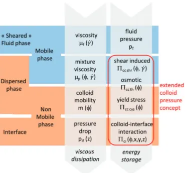
Fig. 2. The SBM-EM model considers thefluid (a mobile phase), the dispersed phase (that can be either mobile or immobile according to the slipping velocity) and the interface (an immobile phase). Frictions leading to viscous dissipation are accounted for through thefluid and the particle-induced viscosity and the colloid mobility, m, when slipping conditions exit. The momentum energy leading to energy storage in the different phases are accounted for through generalized colloid pressure that can include the osmotic pressure contribution (function of the volume fraction), the compressive yield stress, the shear-induced pressure (function of the shear) and the colloid interfacial pressure (function of the energy map and then of the spatial coordinates).
Fig. 3. Representation (on the left) of the 2D energy map induced by a charged pore (simulation realised by Y. Hallez according toHallez et al. (2014)). For the case study of this paper, only the 1D case is treated which corresponds to the transfer on the pore axis or through a dense membrane. The interfacial pressure (on the right) is a function of z with a positive interfacial pressure inside the membrane, MB, and progressive variations in exclusion layers, EX. The interfacial pressure is zero in the surrounding concentration polarization layers, PL.
where um represents the permeate flux and is constant along z (according to Eq.(22)). The interfacial pressure will then be a function of z: the non-dimensional distance on the axis normal to the membrane surface.
A continuous differentiable function is used to depict the variation of the interfacial potential along z (the function is given inS4 of the Supplementary information). The non-dimensional maximum value of the function,V
kT
Π
p icmax, is taken at –ln(0.1) which leads to a value of 0.1
for the partition coefficient according to the Eq.(25). The interfacial pressure variation allows then to define polarization layers, PL (where interfacial pressure is zero), the exclusion layer, EX (where the gradient of interfacial pressure is localized) and the membrane layer, MB (where the interfacial pressure is maximum). All of the simulation data, together with the osmotic pressure (fully described inBacchin et al. (2006)) are given in theSupplementary information (S4).
To perform simulations, the boundary conditions are classically defined with a constant volume fraction at the inlet, ϕ0=0.001, and a non-diffusive flux at the outlet. The initial condition is a neil volume fraction all along z. The simulations are coded with python language (Canopy Enthought package) by using the fipy partial differential equation solver (Guyer et al., 2009). The full code is available on request.
The results of the transient simulation for a mixture velocity, um, of 10−5m/s are presented in Fig. 4. These conditions correspond to a Péclet number of 0.46, when defined as u δm bl/D0 with δbl being the
thickness of the boundary layer thickness (10−6m) and D
0, the
diffusion coefficient in dilute conditions (2.18·10–11m2/s). The simu-lation are continuously depicting the polarization layer formation induced by the membrane surface exclusion, the convection-diffusion balance inside the membrane and the exclusion at the extremities of the membrane. At steady state, the volume fraction is, ϕp=0.256, in the permeate side leading to a solute retention,R= 1 −ϕϕp=0.744
0 .
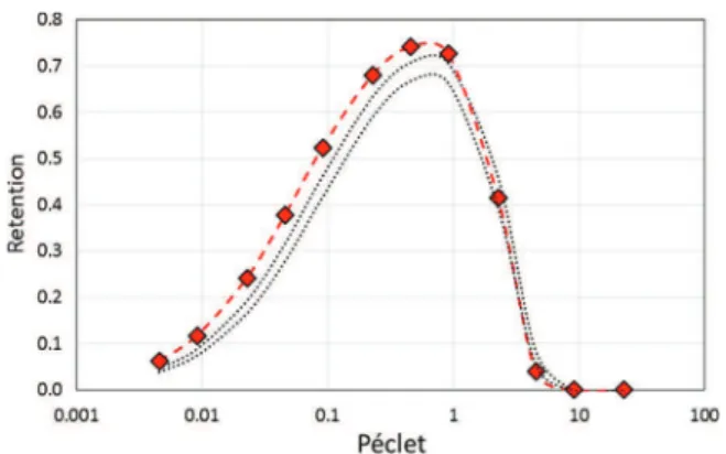
The description of the transfer through a membrane is classically described by an analytical relationship (seeS5 of the Supplementary information), based on (1) the coupling of a convection-diffusion balance inside the membrane, and (2) the coupling in the boundary layer, and (3) a partition coefficient (with a concentration discontinu-ity) between the membrane and the outside solution. Simulations have been performed for different permeate velocities (or Péclet number) and the solute retention at steady state is compared to this analytical model inFig. 5. The analytical model appears with two dashed lines due to the fact that the Pe numbers used in the analytical equation can
be written differently depending on whether the exclusion layers are accounted for in the membrane thickness or in the boundary layer thickness. The simulation results are close to the result obtained with the analytical expression. The small discrepancies could result from the way the partition is accounted for: with a ramp of potential in the simulation and with a discontinuity in the concentration profile in the analytical expression. The effect of the slope of the ramp, that could explain the facilitated transfer observed when working with pores that exhibit a conic shape of an hour glass shape (Gravelle et al., 2013; Li et al., 2015), will be further investigated.
Solving of the mass balance (Eq.(18)) with the 1D energy map (Fig. 3) enables a description of the main transport phenomena that occurs through a membrane, with:
– the convection-diffusion balance inside the membrane that explains the increase in the retention for a small Péclet number, usually observed in reverse osmosis process (when the convection enables the reduction of the negative impact of the diffusion on the selectivity)
– the polarization layer in the boundary layer near the interface that leads to a decrease in retention for a higher Péclet number, usually observed in ultrafiltration (when the increase in concentration at the membrane interface favors the transmission of the solute in the permeate).
From the integration of the momentum balance (Eq.(20)), it is also possible to determine the counter pressure that will be opposed to the difference in static pressure. The counter pressure, CP, can be determined by integrating the momentum balance term,
∫
ϕdΠic. Thecounter pressure has been determined for the simulations performed for different Péclet numbers. The results are presented inFig. 6where the counter pressure is plotted as a function of the difference between the maximum of the osmotic pressure in the concentrate and the osmotic pressure in the permeate,Πcc max−Πcc per (that is classically
used for the counter pressure estimation). The values obtained from the integration of the interfacial pressure and from the “bulk” osmotic pressure difference are similar. The discrepancy can be explained from the writing of the counter pressure, CP, obtained through the integra-tion of the momentum balance for the particle phase (Eq. (S3-1)) along the exclusion layers and the membrane layers:
∫
∫
CP= ϕdΠ =∆Π + nF dz
EX MB+ ic cc EX MB+ drag (28)
This relationship links the counter pressure to the osmotic pressure difference and to the drag force along the exclusion and the membrane layers. Assuming the absence of an additional contribution of a compressive yield stressΠcc cys(that could represent the pressure drop
in a deposit layer), the difference in particle pressure,∆Πcc, is mainly
due to the thermodynamic contribution,∆Πcc th. The counter pressure is
Fig. 4. The transient variation of the volume fraction, ϕ, along z (the vertical lines represent the membrane thickness-full lines and the exclusion layers-dashed lines). The simulation are continuously describing the polarization layer formation, the exclusion near the membrane inlet, the convection-diffusion inside the membrane, the exclusion near the membrane outlet and thefiltrate side.
Fig. 5. Membrane retention calculated as a function of the Pe number. The line of symbols represent the simulation results. These results are compared to the ones obtained with an analytical expression, based on a partition coefficient.
therefore linked to the difference in osmotic pressure,∆Πcc th, at the
interfaces between the exclusion and the bulk that are very close to the maximum osmotic pressure and the permeate osmotic pressure (Fig. 4):
∫
ϕdΠ =Π −Π +∫
nF dz EX MB ic cc th max cc th per EX MB drag + + (29)The difference between the calculated counter pressure and the osmotic pressure difference is due to the drag force that can be seen as the out-of-equilibrium contribution to the counter pressure. This contribution highlights the gap with the spontaneous reversible process (due to the osmotic pressure difference) that is valid only if considering a sequence of equilibrium states (quasi-static process) i.e. if the process is carried out sufficiently slowly. The out-of-equilibrium term is linked to the drag force which is accounting for dissipative effects (internal friction); this term is not taken into account when considering the idealized succession of equilibrium states (Peppin et al., 2005). This gap is negative when um< up(for low Péclet numbers) and becomes positive when um> up. The Peclet number for which the curve crosses the bisector can be associated to the critical Péclet number, i.e. when um=up. For lower Peclet number, the discrepancy can be described via a Staverman coefficient,σof 0.8 (when the counter osmotic pressure is written,σ Π( cc max−Πcc per)).
The SBM-EM model can enable having a good description of both the concentration profile and the solute transmission through the membrane (Fig. 5) and the impact of the accumulation on the out-of-equilibrium counter osmotic pressure (Fig. 6). The counter osmotic pressure is therefore explained by the interfacial interaction between the colloids and the interface. These interactions prevent the colloids from leaving the volume, which then lead to a modification of the movement of the particles at the interface that becomes non-isotropic near the interface. The colloids exchange momentum with the interface and a part of this momentum is returned to the dispersed phase (via the energy principle of action and reaction), thus generating additional gradient in colloid pressure. This gradient of particle pressure, induced by the interface, generates a force that is transmitted to thefluid (via the drag force), that result in osmosis. The model can also describe the shear-induced mechanisms and the formation of gel or deposit layer at the membrane surface (Bacchin et al., 2002). Another interesting aspect of this model lies in the fact that the energy map can easily be adapted to describe more complex transfer problems that can be encountered in membrane processes.
6. Conclusions
The concept of the energy map is implemented in the Suspension
Balance Model (SBM) in order to account for transport phenomena due to particle/wall interactions. This Eulerian model can then simulta-neously describe the effect of multibody particle-particle interactions (through the osmotic pressure or the generalized concept of particle pressure) and the particle-wall interactions (through an interfacial pressure relative to the free energy due to the colloid-wall interaction). The interfacial pressure is a key parameter that characterizes the particle/wall interaction: the energy map represents the value of the interfacial pressure spatially. The gradient in the energy map leads to additional terms of transport phenomena (implemented in the mass balance) and of momentum exchange (implemented in the momentum balance). A new set of equation has been established for this full model (SBM-EM). The coupling of the additional new terms enables account-ing for the Boltzmann exclusion of colloids near the interfaces, the presence of heterogeneous criticalflux (when the advection leads to overcome the map energy barrier) and the osmoticflow (through the momentum exchange term). The model is applied for a 1D modeling of the transfer through a membrane. It enables the description of the retention of a solute through a membrane (i.e. through the polarization layer, the exclusion layers and inside the membrane) and the determi-nation of the out-of-equilibrium counter pressure (that can be seen as the direct consequence of the colloid's interaction with the semi-permeable membrane wall). The model is compared to the analytical relationships that exist for 1D problem. At the end, the SBM-EM model enables the representation of the interaction of the colloids with their environment (for example when the dispersion flows in a confined media). The energy map can allow flexibility in incorporating the physical and chemical heterogeneities of the interacting surfaces. It might be of interest to explore the transfer of colloids along or inside real surfaces (being a mosaic of nano or microscale domain with specific interactions).
Acknowledgements
The author thanks Yannick Hallez, Martine Meireles and Pierre Aimar for the fruitful discussions on this modeling.
Appendix A. Supplementary information
Supplementary information associated with this article can be found in the online version at http://dx.doi.org/10.1016/j.ces.2016. 10.024.
References
Agbangla, G.C., Bacchin, P., Climent, E., 2014. Collective dynamics offlowing colloids during pore clogging. Soft Matter 10, 6303–6315.http://dx.doi.org/10.1039/ C4SM00869C.
Al-Obaidi, H., Florence, A.T., 2015. Nanoparticle delivery and particle diffusion in confined and complex environments. J. Drug Deliv. Sci. Technol. 30 (Part B), 266–277.http://dx.doi.org/10.1016/j.jddst.2015.06.017, (In Honor of Prof. Dominique Duchêne).
Bacchin, P., Aimar, P., Sanchez, V., 1995. Model for colloidal fouling of membranes. AIChE J. 41, 368–376.http://dx.doi.org/10.1002/aic.690410218.
Bacchin, P., Espinasse, B., Bessiere, Y., Fletcher, D.F., Aimar, P., 2006. Numerical simulation of colloidal dispersionfiltration: description of critical flux and comparison with experimental results. Desalination 192, 74–81.http://dx.doi.org/ 10.1016/j.desal.2005.05.028.
Bacchin, P., Marty, A., Duru, P., Meireles, M., Aimar, P., 2011. Colloidal surface interactions and membrane fouling: investigations at pore scale. Adv. Colloid Interface Sci. 164, 2–11.http://dx.doi.org/10.1016/j.cis.2010.10.005.
Bacchin, P., Si-Hassen, D., Starov, V., Clifton, M., Aimar, P., 2002. A unifying model for concentration polarization, gel-layer formation and particle deposition in cross-flow membranefiltration of colloidal suspensions. Chem. Eng. Sci. 57, 77–91.http:// dx.doi.org/10.1016/S0009-2509(01)00316-5.
Batchelor, G.K., 1970. The stress system in a suspension of force-free particles. J. Fluid Mech. 41, 545–570.http://dx.doi.org/10.1017/S0022112070000745.
Buscall, R., White, L.R., 1987. The consolidation of concentrated suspensions. Part 1.— The theory of sedimentation. J. Chem. Soc. Faraday Trans. 1: Phys. Chem. Condens. Phases 83, 873–891.http://dx.doi.org/10.1039/F19878300873.
Clausen, J.R., 2013. Using the suspension balance model in afinite-element flow solver. Comput. Fluids 87, 67–78.http://dx.doi.org/10.1016/j.compfluid.2012.12.004, Fig. 6. The counter osmotic pressure deduced from the simulation,∫ϕdΠic, as a function
of the counter osmotic pressure determined through the difference in osmotic pressure between the maximum of the osmotic pressure in the polarization layer and the osmotic pressure in the permeate,Πcc max−Πcc per. The arrow on the dashed line indicates the
(USNCCM Moving Boundaries).
Deboeuf, A., Gauthier, G., Martin, J., Yurkovetsky, Y., Morris, J., 2009. Particle pressure in a sheared suspension: a bridge from osmosis to granular dilatancy. Phys. Rev. Lett., 102.http://dx.doi.org/10.1103/PhysRevLett.102.108301.
Derjaguin, B.V., Churaev, N.V., 1974. Structural component of disjoining pressure. J. Colloid Interface Sci. 49, 249–255.http://dx.doi.org/10.1016/0021-9797(74) 90358-0.
Elimelech, M., Bhattacharjee, S., 1998. A novel approach for modeling concentration polarization in crossflow membrane filtration based on the equivalence of osmotic pressure model andfiltration theory. J. Membr. Sci. 145, 223–241.
Gravelle, S., Joly, L., Detcheverry, F., Ybert, C., Cottin-Bizonne, C., Bocquet, L., 2013. Optimizing water permeability through the hourglass shape of aquaporins. Proc. Natl. Acad. Sci. USA 110, 16367–16372.http://dx.doi.org/10.1073/
pnas.1306447110.
Guyer, J.E., Wheeler, D., Warren, J.A., 2009. FiPy: partial differential equations with python. Comput. Sci. Eng. 11, 6–15.http://dx.doi.org/10.1109/MCSE.2009.52. Hallez, Y., Diatta, J., Meireles, M., 2014. Quantitative assessment of the accuracy of the
poisson–boltzmann cell model for salty suspensions. Langmuir 30, 6721–6729.
http://dx.doi.org/10.1021/la501265k.
Hallez, Y., Gergianakis, I., Meireles, M., Bacchin, P., 2016. The continuous modeling of charge-stabilized colloidal suspensions in shearflows. J. Rheol..http://dx.doi.org/ 10.112/1.4964895, (to be published).
Hoek, E.M.V., Bhattacharjee, S., Elimelech, M., 2003. Effect of membrane surface roughness on colloid-membrane DLVO interactions. Langmuir 19, 4836–4847.
http://dx.doi.org/10.1021/la027083c.
Jacazio, G., Probstein, R.F., Sonin, A.A., Yung, D., 1972. Electrokinetic salt rejection in hyperfiltration through porous materials. Theory and experiment. J. Phys. Chem. 76, 4015–4023.http://dx.doi.org/10.1021/j100670a023.
Jackson, R., 2000. The Dynamics of Fluidized Particles. Cambridge University Press, Cambridge.
Jackson, R., 1997. Locally averaged equations of motion for a mixture of identical spherical particles and a Newtonianfluid. Chem. Eng. Sci. Math. Model. Chem. Biochem. Process. 52, 2457–2469.http://dx.doi.org/10.1016/S0009-2509(97) 00065-1.
Jiang, S., Cao, Z., 2010. Ultralow-fouling, functionalizable, and hydrolyzable zwitterionic materials and their derivatives for biological applications. Adv. Mater. 22, 920–932.
http://dx.doi.org/10.1002/adma.200901407.
Kemps, J.A.L., Bhattacharjee, S., 2005. Interactions between a solid spherical particle and a chemically heterogeneous planar substrate. Langmuir 21, 11710–11721.
http://dx.doi.org/10.1021/la051292q.
Leighton, D., Acrivos, A., 1987. The shear-induced migration of particles in concentrated suspensions. J. Fluid Mech. 181, 415–439.http://dx.doi.org/10.1017/
S0022112087002155.
Lhuillier, D., 2011. Thermodiffusion of rigid particles in pure liquids. Phys. Stat. Mech. Appl 390, 1221–1233.http://dx.doi.org/10.1016/j.physa.2010.12.010.
Lhuillier, D., 2009. Migration of rigid particles in non-Brownian viscous suspensions. Phys. Fluids (1994-Present) 21, 023302.http://dx.doi.org/10.1063/1.3079672. Li, Y., Borujeni, E.E., Zydney, A.L., 2015. Use of preconditioning to control membrane
fouling and enhance performance during ultrafiltration of plasmid DNA. J. Membr. Sci. 479, 117–122.http://dx.doi.org/10.1016/j.memsci.2015.01.029.
Mason, T.G., Lacasse, M.-D., Grest, G.S., Levine, D., Bibette, J., Weitz, D.A., 1997. Osmotic pressure and viscoelastic shear moduli of concentrated emulsions. Phys. Rev. E 56, 3150–3166.http://dx.doi.org/10.1103/PhysRevE.56.3150. Miller, R.M., Singh, J.P., Morris, J.F., 2009. Suspensionflow modeling for general
geometries. Chem. Eng. Sci. 64, 4597–4610.http://dx.doi.org/10.1016/ j.ces.2009.04.033.
Morris, J.F., Boulay, F., 1999. Curvilinearflows of noncolloidal suspensions: the role of normal stresses. J. Rheol. (1978-Present) 43, 1213–1237.http://dx.doi.org/ 10.1122/1.551021.
Noetinger, B., 1989. A twofluid model for sedimentation phenomena. Phys. Stat. Mech. Appl. 157, 1139–1179.http://dx.doi.org/10.1016/0378-4371(89)90037-X. Nott, P.R., Brady, J.F., 1994. Pressure-drivenflow of suspensions: simulation and theory.
J. Fluid Mech. 275, 157–199.http://dx.doi.org/10.1017/S0022112094002326. Nott, P.R., Guazzelli, E., Pouliquen, O., 2011. The suspension balance model revisited.
Phys. Fluids (1994-Present) 23, 043304.http://dx.doi.org/10.1063/1.3570921. Peppin, S.S.L., Elliott, J. a.W., Worster, M.G., 2005. Pressure and relative motion in
colloidal suspensions. Phys. Fluids (1994-Present) 17, 053301.http://dx.doi.org/ 10.1063/1.1915027.
Shen, C., Wang, F., Li, B., Jin, Y., Wang, L.-P., Huang, Y., 2012. Application of DLVO energy map to evaluate interactions between spherical colloids and rough surfaces. Langmuir 28, 14681–14692.http://dx.doi.org/10.1021/la303163c.
Vollebregt, H.M., van der Sman, R.G.M., Boom, R.M., 2010. Suspensionflow modelling in particle migration and microfiltration. Soft Matter 6, 6052.http://dx.doi.org/ 10.1039/c0sm00217h.
Wijmans, J.G., Nakao, S., Van Den Berg, J.W.A., Troelstra, F.R., Smolders, C.A., 1985. Hydrodynamic resistance of concentration polarization boundary layers in ultrafiltration. J. Membr. Sci. 22, 117–135. http://dx.doi.org/10.1016/S0376-7388(00)80534-7.