O
pen
A
rchive
T
OULOUSE
A
rchive
O
uverte (
OATAO
)
OATAO is an open access repository that collects the work of Toulouse researchers and
makes it freely available over the web where possible.
This is a publisher’s version published in :
http://oatao.univ-toulouse.fr/
Eprints ID : 18391
To link to this article : DOI:
10.1051/alr/2017003
URL :
https://doi.org/10.1051/alr/2017003
To cite this version :
Drouineau, Hilaire and Bau, Frédérique and
Alric, Alain and Deligne, Nicolas and Gomes, Peggy and Sagnes,
Pierre Silver eel downstream migration in fragmented rivers: use of
a Bayesian model to track movements triggering and duration.
(2017) Aquatic Living Resources, vol. 30 (n° 5). pp. 1-19. ISSN
0990-7440
Any correspondence concerning this service should be sent to the repository
administrator:
[email protected]
R
ESEARCHA
RTICLESilver eel downstream migration in fragmented rivers: use of a
Bayesian model to track movements triggering and duration
★Hilaire Drouineau
1,2,*, Frédérique Bau
1,2, Alain Alric
2, Nicolas Deligne
1,2, Peggy Gomes
2and Pierre Sagnes
21 Irstea UR EABX, 50 avenue de Verdun, 33612 Cestas Cedex, France
2 Pôle Écohydraulique ONEMA-Irstea-INP, Allée du professeur Camille Soula, 31400 Toulouse, France
Received 26 July 2016 / Accepted 27 January 2017
Abstract – Obstacles in rivers are considered to be one of the main threats to diadromous fish. As a result of the recent collapse of the European eel, the European Commission introduced a Regulation, requiring to reduce all sources of anthropogenic mortality, including those caused by passing through hydropower turbines. Improving knowledge about migration triggers and processes is crucial to assess and mitigate the impact of obstacles. In our study, we tracked 97 tagged silver eels in a fragmented river situated in the Western France (the River Dronne). Using the movement ecology framework, and implementing a Bayesian state-space model, we confirmed the influence of river discharge on migration triggering and the distance travelled by fish. We also demonstrated that, in our studied area, there is a small window of opportunity for migration. Moreover, we found that obstacles have a significant impact on distance travelled. Combined with the small window, this suggests that assessment of obstacles impact on downstream migration should not be limited to quantifying mortality at hydroelectric facilities, but should also consider the delay induced by obstacles, and its effects on escapement. The study also suggests that temporary turbines shutdown may mitigate the impacts of hydropower facilities in rivers with migration process similar to those observed here.
Keywords: Anguilla anguilla / Silver eel / Migration delay / River fragmentation / Movement ecology / State-space model
1 Introduction
Movement plays a fundamental role in a large variety of biological, ecological and evolutionary processes (Nathan, 2008). Migration is a specific type of movement particularly prevalent among taxa (Wilcove and Wikelski, 2008). The phenomenon is defined by Dingle (1996) as a continuous, straightened out movement not distracted by resources. Contrary to other movements (mainly foraging and dispersion (Jeltsch et al., 2013)), migration is generally a response to environmental cues such as temperature or photoperiod, and not only to fluctuations in resources and the availability of mates (Dingle, 2006). Because of their sensitivity to habitat degradation, overexploitation, climate change, and obstacles to migration, most migratory species are in decline (McDowall, 1999;Sanderson et al., 2006;Berger et al., 2008;Wilcove and Wikelski, 2008). Consequently, improving knowledge about
animal migration and its relationship with the rest of the life cycle is of high scientific importance.
Diadromous fish are species that migrate between sea and fresh water during their life cycle (Myers, 1949;McDowall, 1968). Three types of diadromy have been described (McDowall, 1988): (i) catadromous species, which spawn in the sea but spend most of their growth phase in continental waters, (ii) anadromous species, which spawn in continental waters but spend most of their growth phase at sea and (iii) amphidromous species, which undergo non-reproductive migration between fresh water and sea during their growth phase. Populations of most diadromous fish species are currently in decline (Limburg and Waldman, 2009). Obstacles to migration, such as dams, are considered to be one of the main threats to those fish species (Limburg and Waldman, 2009). They are also seen as the root cause of some population extinctions or their keeping in confined areas within river catchments (Porcher and Travade, 1992; Kondolf, 1997;
Coutant and Whitney, 2000;Larinier, 2001;Fukushima et al., 2007). Obstacles can have a large variety of impacts. Direct mortality as a result of water turbines has been widely studied and quantified (Blackwell et al., 1998;Williams et al., 2001;
★
Supporting information is only available in electronic form at
www.alr-journal.org.
* Corresponding author:[email protected] EDP Sciences2017
DOI:10.1051/alr/2017003
Living
Resources
Available online at:
Čada et al., 2006;Buchanan and Skalski, 2007;Dedual, 2007; Welch et al., 2008;Travade et al., 2010). However, obstacles can have many other consequences (Budy et al., 2002), including stress, disease, injury, increased energy costs, migration delay (Muir et al., 2006; Caudill et al., 2007;
Marschall et al., 2011) overpredation, and overfishing (Briand et al., 2003;Garcia De Leaniz, 2008) of populations that often suffer intense exploitation (McDowall, 1999). In view of this, understanding diadromous fish migration is a critical issue for conservation (McDowall, 1999) and can inform biodiversity policy (Barton et al., 2015).
This is especially true for catadromous European eels (Anguilla anguilla), which spawn in the Sargasso Sea (Schmidt, 1923; Tesch, 2003) and grow in European continental waters after a few years long larval drift (Bonhommeau et al., 2009). Leptocephali metamorphose into glass eels when they arrive on the continental shelf (Tesch, 2003). Glass-eels then colonise continental waters, where they become pigmented yellow eels and remain during their growth phase, which lasts several years. Colonisation tactics are largely plastic, and eels are able to use a variety of habitats, ranging from estuaries and lagoons to upstream rivers (Daverat et al., 2006). After a period varying between 3 and 15 years in duration, yellow eels metamorphose into silver eels, migrate back to the sea, and travel across the ocean to the Sargasso Sea (van Ginneken and Maes, 2005). River fragmentation can therefore impact both the upstream migration of glass-eels (Briand et al., 2005;Mouton et al., 2011;Piper et al., 2012;
Drouineau et al., 2015) and downstream migration of silver eels (Acou et al., 2008;Piper et al., 2013;Buysse et al., 2014). As a result of a population collapse (Dekker et al., 2003,2007), observed on both recruitment (Castonguay et al., 1994;
ICES, 2014; Drouineau et al., 2016) and spawning biomass (Dekker, 2003), the European Commission introduced Council Regulation N°1100/2007, which requires a reduction in all sources of anthropogenic mortality, including death caused when passing through hydroelectric turbines during down-stream migration.
Three main types of studies have been carried out to improve knowledge of silver eel downstream migration. Many have focused on the behaviour of silver eels passing downstream through hydroelectric power stations to estimate mortality (Boubée and Williams, 2006;Carr and Whoriskey, 2008;Travade et al., 2010;Pedersen et al., 2012) or to improve mitigation solutions (Gosset et al., 2005;Russon and Kemp, 2011;Calles et al., 2013). Some studies have tracked silver eels along fragmented watercourses to estimate escapement (Haraldstad et al., 1985; Jansen et al., 2007; Acou et al., 2008;Breukelaar et al., 2009;Verbiest et al., 2012;Piper et al., 2013;Marohn et al., 2014; Mccarthy et al., 2014; Reckordt et al., 2014). Other studies have focused on migration triggered by environmental factors, to predict migration activity and especially peaks of migration, and consequently when to shutdown turbines (Vøllestad et al., 1986;Durif et al., 2008;
Durif and Elie, 2008; Trancart et al., 2013). One common aspect in these previous studies is that they make use of the same two types of data: telemetric tracking or daily abundance estimates (through either catching or counting). Moreover, the three key issues (mortality at hydro-electric power stations, escapement, and triggers for migration) are generally addressed separately.
The movement ecology framework (Nathan et al., 2008) appears to be an appropriate way of simultaneously studying both triggers of migration and the impact of obstacles on escapement. Movement ecology is a specific field of ecology focusing on organism movements (Nathan, 2008;Nathan et al., 2008). More specifically, it examines the interplay between an individual internal state, its motion capacity, its navigation capacity and the environment. This interplay is addressed through movement analysis. Several types of questions may be addressed (Nathan et al., 2008): (i) why organisms move, (ii) how they move, (iii) where and (iv) when they move, (v) how the environment influences those movements, and (vi) how those components interact together (Nathan et al., 2008). Depending on their objectives, studies may focus on one or several of those questions (Holyoak et al., 2008).
The development of tracking methods during the 1990s revolutionized behavioural and movement ecology (Jonsen et al., 2003;Cagnacci et al., 2010). Satellite tags (Safi et al., 2013), satellite based monitoring systems (Vermard et al., 2010;Bez et al., 2011;Joo et al., 2013), and acoustic tags with positioning algorithms (Berge et al., 2012) now provide fine-scale temporal and spatial position data relating to fish, mammals, birds, boats, etc. Different tools have been developed to analyse such trajectory data. Among these tools are state-space models (SSM) (Patterson et al., 2008;Jonsen et al., 2013) and, more specifically, Hidden Markov Chain models (Joo et al., 2013). These are based on two distinct sub-models. The state model describes the evolution of animal states across different (generally discrete) time-steps. The observation model describes the link between unobserved states and observations. In movement ecology, states are generally a position and type of behaviour, while observations may be an estimation of position, speed or any other monitored parameter providing information on movement (Jonsen et al., 2013). In their synthesis,Patterson et al. (2008)
detail the advantages of SSM in movement ecology. SSM enables statistical inference, accounting for various types of uncertainty. It provides many interesting outputs: state probabilities (spatial location and duration of specific behaviours), process model parameters for each state/ behaviour, and observation model parameters. Also, the flexibility of SSM allows the effects of environmental factors on state/behaviour transition to be taken into account. Consequently, SSMs are relevant tools to address each of the questions of movement ecology.
In this paper, we used the movement ecology framework to study silver eel migration and assess the impact of obstacles in a highly fragmented river in southwest France. More specifically, we developed a single integrated state-space model to (i) analyse the effects of different environmental factors on migration triggering and derive the corresponding environmental suitability envelops, (ii) quantify the impact of river flow on migration speed, and (iii) quantify the impact of obstacles on this speed. We analysed the implications of the results from a conservation point of view. The model was applied to data relating to 68 eels (among 97 tagged) tracked along 90 kilometres of the watercourse, covering three successive migration seasons. Our study illustrates how a state-space model may respond to the different movement ecology questions listed byNathan et al. (2008), specifically “when do they move?” (environmental triggering) and
“how do they move?” (influence of discharge and weirs on migration speed).
2 Material and methods
2.1 Data
2.1.1 Study site: Dronne River
The river Dronne is a 200-kilometer long low land plain river located in the southwest of France (Fig. 1). Its watershed covers 2816 km2. It flows into the river Isle, a tributary of the Dordogne River, about 80 km from the Bec d'Ambès, where the Dordogne and Garonne rivers flow into the Gironde estuary. It is one of the 10 “index rivers” identified in the French Eel Management Plan (Anonymous, 2010) in which specific efforts are made to quantify yearly eel recruitment and escapement. Oceanic-type rainfall is observed, with a 45 years average discharge of 19.6 m3/s at Bonnes (Table 1). The study site covers approximately 90 km
along the downstream section of the river (Fig. 1). The river is highly fragmented, with 91 obstacles referenced in the French obstacles inventory (ROE® database, finalized version 5.0, http://www.onema.fr/REFERENTIEL-DES-OBSTACLES-A-L), i.e. one obstacle every 2.2 km (every 2.1 km on the studied section) on average. Most obstacles correspond to old mill weirs, with a waterfall of less than two meters. Many obstacles are now disused, although a few of them (7 of the 43 obstacles located in the study area) are still used for hydroelectricity production.
2.1.2 Environmental data
The study took place during three successive eel downstream migration seasons: 2011–2012, 2012–2013, 2013–2014.
Daily river flow data were obtained from the French “Banque Hydro” (website: http://www.hydro.eaufrance.fr). Discharge was collected in three different stations of the studied area, however only discharge measured at Bonnes
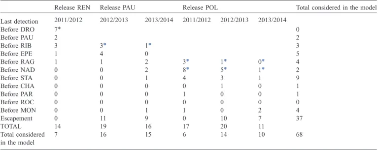
Dronne Isle Dordogne Garonne Gironde Atlantic Ocean 1°W 0° 1°E 45°N 45.5°N 0 km 25 km Bordeaux CHA EPE DRO MON NAD PAR PAU RAG RIB ROC STA POL EPA PAU POL REN 0 km 10 km release obstacles receivers
Fig. 1. Maps of the Dronne River. Black circles represent obstacles referenced in the French ROE database. White circles represent thefixed radio-telemetry receivers (Table 2). Diamonds represent eels release locations (Table 2). River flow is measured at Bonnes, immediately downstream the radio-telemetry receiver RAG. Physico-chemical parameters were monitored closed to the ATS receivers PAU, NAD and MON. Acronyms refer to towns or sites. REN, Renamon; DRO, Maison de la Dronne; PAU, Moulin de la Pauze; RIB, Ribérac; EPE, Epeluche; POL, Moulin de Poltot; RAG, Ragot; NAD, Nadelin; STA, Saint-Aulaye; CHA, Chamberlanne; PAR, Parcoul; ROC, La Roche-Chalais; MON, Monfourat.
(just downstream RAG, Figs. 1 and 2 – Table 1) was considered for this study, since the three series were perfectly correlated.
Mean daily air temperatures were provided by Météo-France®and collected in Saint-Martial, a station located a few kilometres from Bonnes (Figs. 1and2).
Table 1. River discharge characteristics at Bonnes monitoring station, measured from 1970 to 2014 for the entire year (first column) and for the months from October to May (second column), which correspond to the tracking period. Q99, Q97.5, Q95, Q90, Q80, Q75 correspond to daily flows extracted from flow duration curve and exceeded 99%, 97.5%, 95%, 90%, 80%, 75% of the time respectively.
1970–2014 (whole year) 1970–2014 (Oct–May) 2011–2012 (Oct–May) 2012–2013 (Oct–May) 2013–2014 (Oct–May)
Mean 19.6 25.2 14.7 26.9 34.9 Median 12.1 17.6 10.4 22.1 28.3 Q75 24.2 30.9 15.8 31.4 44.9 Q80 28.4 35.8 18.0 36.0 48.2 Q90 42.5 51.5 28.4 59.0 71.4 Q95 59.9 72.0 40.1 70.6 88.3 Q97.5 83.0 97 66.4 81.0 99.9 Q99 115.0 129 114.0 103.9 110.1
Nov Jan Mar May
0
5
0
100
150
Nov Jan Mar May
0
5
0
100
150
Nov Jan Mar May
0 5 0 100 150 Q
(
m 3 s)
2011−2012 2012−2013 2013−2014Nov Jan Mar May
− 1 0 −5 0 5 1 0 1 5 2 0
Nov Jan Mar May
− 1 0 −5 0 5 1 0 1 5 2 0
Nov Jan Mar May
− 1 0 −5 0 5 1 0 1 5 2 0 T°C
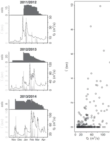
Fig. 2. Daily discharge (first line ! solid black line) and air temperature (second line ! solid black line) during the three eel downstream migration seasons (in columns). Solid grey lines indicated monthly means over 45 years (flow) and 30 years (air temperature monitored in Bergerac, a station located 40 km from our studied area which has a longer time-series). For river flow, dashed lines represent the average discharge over 45 years long period, and the dotted line represents the 2-year flood.
Water conductivity (WTW TetraCon®
), turbidity (WTW VisoTurb®), temperature and dissolved oxygen (WTW FDO® 700 IQ) were collected every hour in three stations (PAU, NAD and MON !Fig. 1). Because strong correlations were observed between environmental variables (Spearman corre-lation coefficients: 0.90 between discharge and turbidity; 0.80 between water temperature and air temperature, 0.62 between air temperature and oxygen), we restricted the dataset to 5 variables: average daily river discharge (Q), relative variation of average daily river discharge (DQ measured as discharge at day d minus discharge at day d ! 1 divided by the discharge at time d ! 1), daily average air temperature (Tair), squared
average daily discharge (Q2), and squared average temperature (Tair2)). Using both factor and squared factors allow mimicking
dome-shaped environmental windows (i.e. a nonlinear relationship passing through a maximum). We chose to use discharge and air temperature because (i) they do not present any gaps contrary to other variables and (ii) those two variables are easily accessible in most rivers. Though less correlated (Spearman correlation coefficient 0.41 between conductivity and air temperature); we did not consider conductivity because records displayed abrupt and unexplainable changes (perhaps due to hydropower operations), timely inconsistent between the three monitoring stations, therefore we considered they were not reliable enough. We also tested relative variation of daily discharge because increasing discharge phase tends to be more favourable than decreasing discharge phase for eel migration (Haro, 2003). The 5 variables are summarized in
Table 2.
The three migration seasons were hydrologically con-trasted, with a first season of low run-off compared to the reference period (1970–2014), and two seasons with more intense discharges (Table 1 and Fig. 2). This contrast was visible both in terms of average discharge (14.7 m3/s in 2011/ 2012 versus 26.9 and 34.9 m3/s in the two following seasons !
Table 1) and in the number of discharge peaks (three short peaks in 2011/2012 versus 5 peaks of longer duration in the two following seasons !Fig. 2). The first migration season was also characterised by a period of very low temperature in January and February.
2.1.3 Fish sampling and tracking
Fish were collected during moderate discharge events in two filter traps incorporated in two old mills (similar to the description byTesch (2003)) located in station REN and POL (Fig. 1). Traps were visited every 12 hours and caught eels were then placed in a tank supplied with river water. Eels were tagged according to the protocol proposed byBaras and Jeandrain (1998)that had already been successfully used by
Travade et al. (2010) and Gosset et al. (2005). Eels were anaesthetized in a solution of acetyleugenol (∼1.1 mL/L),
measured, and weighed. Their head lengths and heights, eyes (vertical and horizontal lengths) and pectoral fins were measured and their stages of maturity was checked according toDurif et al. (2005)andAcou et al. (2005)indices. A coded ATS (Advanced Telemetry System) radio-transmitter with a pulse rate of 45 ppm (F1820 frequency 48–49 MHz, length 43 mm, diameter 12 mm, weight 8 g, minimum battery capacity 95 days or F1815 frequency 48–49 MHz, length 36 mm, diameter 12 mm, weight 7 g, minimum battery capacity 65 days) was implanted in the body cavity by surgical incision as described byBaras and Jeandrain (1998). Intracoelomic implantation limits the risk of tag expulsion (Bridger and Booth, 2003;Brown et al., 2011) and has a more limited impact on fish behaviour and survival (Koeck et al., 2013).Baras and Jeandrain (1998)had specifically validated the tag retention for eels whileWinter et al. (2005)confirmed good tag retention and survival, and limited behavioural impact using intracoelomic implantation. The advocated threshold of 2% (weight of tag in air/weight of fish) was carefully checked (Winter, 1983; Brown et al., 1999) (see alsoJepsen et al., 2005;Moser et al., 2007for anguiliforms). High tag emission rates (45 ppm) were required to ensure efficient detections rates by autonomous receivers but decreased drastically batteries life. Consequently, we had to tag fishes that were expected to move fairly soon after tagging, that's why we used eels caught by a filter trap (this type of trap mainly catch active migrant). All eels fulfilling the 2% ratio rule were tagged except a few individuals that had been injured during the catching process (other individuals were in good health). According to Durif et al. (2005) and Acou et al. (2005), they were all silver eels (Table S1) and consequently expected to migrate in the short terms.
Similarly toGosset et al. (2005), an exit hole was made for the antenna with a hollow needle through the body wall 2 cm behind the incision and closed up with cyanoacrylate adhesive. The incision was then closed up using a monofilament absorbable suture (Ethicon PDS®
II 2-0, 3/8c vc tr 24 mm Z453H model) and a cyanoacrylate adhesive with antimicro-bial effect (3MTMVetbondTM Tissue Adhesive) to speed up
healing (<10 s). Following a veterinary advice, a broad course and long-lasting antibiotics was also injected to reduce the risk of infection (Shotapen 1.0 mL/kg). Eels were released a few hours after surgery in three different places (Fig. 1). The protocol was developed to limit the time between eel catch and release and to limit the transportation between catch point and release point in order to limit behavioural biases due to tagging or infection in holding tanks. More specifically, all the work was designed to respect animal welfare and to minimize suffering. Finally, 97 silver eels were tagged and tracked during the 3 migration seasons. Given that their total lengths were largely greater than 45 cm, we can assume that they were Table 2. Characteristics of the 5 environmental variables during the whole three migration seasons.
Q (m3s!1) Q2(m3s!1)2 Tair (°C) Tair2(°C2) DQ (%)
Range (min; max) 1.94; 144.00 3.76; 20736.00 !8.3; 23.9 0.04; 571.21 !36.4; 170.4
Mean 25.49 1180.61 9.7 120.6 2.2
all females (Tesch, 1991; Durif, 2003). Their complete biometry is presented inSupplementary Material.
Eleven R4520 ATS®
autonomous receivers with low frequency antenna loop were installed at different points along the river to detect passing fish (Fig. 1 and Table 3). The receivers were listening continuously the only frequency used with a fast setting (2 s time out, a 10 s scan time and 1 mn store rate). This setting combined with a full gain setting that provides 200 m detection range (validated by field tests) ensured that no fish were missed. In addition, active tracking was carried out on a weekly basis to try locating eels more precisely. Unfortunately, the river is not easily accessible along the whole study so active tracking provided sparse data that were not included latter in the study, except to check whether the transmitters were still working. It also confirmed that autonomous receivers had successfully detected all passages.
Radiotracking had already been used to study eel downstream migration (Durif, 2003; Winter et al., 2006;
Travade et al., 2010) and had proved efficient in freshwater systems such as ours. It is well suited in shallow waters and when working close to river obstacles because not sensitive to turbulences contrary to many acoustic systems. Moreover, active tracking can be carried out by car (in a fragmented river such as the Dronne river, a tracking by boat required by acoustic telemetry would be impossible).
For each day t and each tagged eel f, we calculated the distance between the most downstream detection before the end of day t and the most downstream detection recorded before the end of day t ! 1. This indicator, denoted I(t,f), gave a rough approximate of the distance travelled each day t by fish f. The daily average over all eels still in the studied area at time t is denoted IðtÞ.
2.2 Model
A state-space model was developed to analyse our results. It is based on a state-model that describes migration triggering and an observation model that describes fish movement (Fig. 3).
2.2.1 Behavioural states transitions and migration triggering
The model has a daily time-step. In each time-step t, a fish f can be in three different unobserved states S(f,t): 1 pause, 2 active migrant, 3 definitive stop (either mortality or definitive withdrawal). In the first state, fish are not moving and are waiting for favourable conditions to migrate. In the second state, fish are actively migrating (i.e. migrating downstream) and will continue to move as long as conditions are favourable. In the third step, fish have definitively abandoned migration or are dead.
State at time step t is assumed to follow a Markovian process: the state at time t depends only on the state at time t!1 and vector of transition probabilities which depend mainly on environmental conditions (transition to state 3 is considered to be independent Fig. 3. Structure of the state-space model illustrating the influence of environmental conditions on the internal behavioural state and their links with eels movements and resulting observations.
Table 3. Relative positions of the different monitoring stations (Fig. 1). Stations Distance from
previous site (km)
Distance from REN release point (km)
Distance from PAU release point (km)
Distance from POL release point (km)
Number of obstacles from previous station
REN 0 – – DRO 8.2 8.2 – – 5 PAU 7.4 15.6 0 – 4 RIB 7.3 22.9 7.3 – 3 EPE 5.7 28.6 13 – 6 POL 10.3 38.9 23.3 – 4 RAG 1.2 40.1 24.5 1.2 1 NAD 8.2 48.3 32.7 9.4 5 STA 6.9 55.2 39.6 16.3 3 CHA 8.5 63.7 48.1 24.8 5 PAR 2.1 65.8 50.2 26.9 1 ROC 10.1 75.9 60.3 37 4 MON 12.8 88.7 73.1 49.8 2
of environmental conditions and may be due to predation, diseases, etc.), through a categorical distribution:
Sðf ; tÞ ∼ CatðfqSðf ;t!1Þ;1ðtÞ; qSðf ;t!1Þ;2ðtÞ; qSðf ;t!1Þ;3ðtÞgÞ; ð1Þ
qi,jdenotes the probability of switching from state i to state j.
Consequently, {qS (f,t!1),1(t) , qS (f,t!1),2(t) , qS (f,t!1),3(t)} is a
vector that contains the probabilities that fish f switches to each possible state given that it was in state S (f, t ! 1) at time step t! 1. Those probabilities are assumed to be a function of environmental conditions: q1;2ðtÞ ¼ ð1 ! peÞ ' 1 1 þ exp !msþ 〈 a!!;sd !!Þ 〉Eðt " # 0 B @ 1 C A; ð2Þ q1;1ðtÞ ¼ ð1 ! peÞ ' ð1 ! q1;2ðtÞÞ; ð3Þ q2;1ðtÞ ¼ ð1 ! peÞ ' 1 1 þ exp !mwþ 〈 a!!;w !!Þ 〉Eðt " # 0 B @ 1 C A; ð4Þ q2;2ðtÞ ¼ ð1 ! peÞ⋅ð1 ! q2;1ðtÞÞ; ð5Þ q1;3ðtÞ ¼ q2;3ðtÞ ¼ pe; ð6Þ q3;3ðtÞ ¼ 1; ð7Þ q3;1ðtÞ ¼ q3;2ðtÞ ¼ 0; ð8Þ
with EðtÞ!!! a vector that contains the environmental factors at time step t.
The table of environmental factors was previously scaled and centred to decrease the correlation between regression parameters (Bolker et al., 2013). a! ands !!aw denote the
vector regression coefficients associated with each environ-mental factor while ms and mw denote the intercept in the
regression between transition probabilities and environmen-tal factors. 〈 A!;!B 〉 denotes the inner product between vectors A!and B!. Finally, pedenotes the daily probability of
definitive abandon (a fish that will definitively not move anymore).
Equations(2)(respectively(4)) means that probability for a fish to switch from state pause to active migrant (respectively active migrant to pause), given it has not definitively abandoned, is similar to a logistic regression of environmental conditions (with intercept m and regressions coefficients a). Equations(3)(respectively equation(5)) is the probability that a fish remains in state 1 (respectively (2)) and is the complement of equation (2) (respectively (4)). Equation 6
mean that the probability to switch to state 3 is constant through time, i.e. do not depend on initial state nor on environmental condition, while equations(7)and(8)mean that a fish in state 3 always remain in state 3.
2.2.2 Movement and observation model
Considering that eel migration speed increases with water velocity, and since water velocity increases as a function of river flow (Leopold and Maddock, 1953), we assumed that the average theoretical distance that an actively migrating fish would travel within 24 hours at time step t without any obstacles Lth(t), was dependent on flow conditions:
LthðtÞ ¼ exp½mmigþ amig⋅logðQðt ! 1ÞÞ+; ð9Þ
with exp(mmig) the distance that an eel would travel in absence
of discharge and expðamig⋅logðQðt ! 1ÞÞÞ the influence of the
water velocity on this distance.
We defined a reach as a portion of the studied area between two successive autonomous receivers. For each day, we know exactly in which reach each eel is located because autonomous receivers were settled to detect all fish passages. Fish movement is modelled through a reach transition matrix composed of the daily transition probability of moving from a reach r1to a reach r2. To simplify the computation of the reach
transition matrix, we assumed that fish were located at the middle of the departure reach at the beginning of each time-step, which is a usual approximation for growth transition matrix (Sullivan et al., 1990; DeLong et al., 2001). We denote dr1;r2the maximum distance that a fish has travelled to
move from reach r1to reach r2. Similarly, we denote nbr1;r2the
maximum number of weirs that a fish must pass through in order to move from reach r1to reach r2. dr1;r2 and nbr1;r2 are
directly calculated usingTable 3.
Assuming that passing an obstacle acts as a penalty equivalent to w kilometres, and that the effective distance covered by an eel in 24 hours follows a lognormal distribution, we can then compute the transition probability to move from a reach r1to a reach r2: pr1;r2ðtÞ ¼ 0 if r1<r2 ∫dr1;r2þw ' nbr1;r2 0 1 2 ' s2 m ' ffiffiffiffiffiffiffiffiffiffiffiffiffiffiffiffiffi ð2 ' pÞ p ' e! 1 2' ðx!lnðLðtÞÞsm Þ 2 if r1¼ r2≠11 ∫dr1;r2þw ' nbr1;r2 dr1;r2!1þw ' nbr1;r2!1 1 2 ' s2 m ' ffiffiffiffiffiffiffiffiffiffiffiffiffiffiffiffiffi ð2 ' pÞ p ' e! 1 2' ðx!lnðLðtÞÞsm Þ 2 if r2>r1and r2≠11 ∫þ∞ dr1;r2!1þw ' nbr1;r2!1 1 2 ' s2 m ' ffiffiffiffiffiffiffiffiffiffiffiffiffiffiffiffiffi ð2 ' pÞ p ' e! 1 2' ðx!lnðLðtÞÞsm Þ 2 if r2>r1and r2¼ 11 1 if r1¼ r2¼ e 8 > > > > > > > > > > > > > > > < > > > > > > > > > > > > > > > :
ð10Þ
with r1and r2a reach index (1: DRO ! PAU, 2: PAU ! RIB,
3: RIB ! EPE, 4: EPE ! RAG, 5: RAG ! NAD, 6: NAD ! STA, 7: STA ! CHA, 8: CHA ! PAR, 9:PAR ! ROC, 10: ROC ! MON, 11: escaped ! seeTable 3andFig. 1)
The observed transition from reach r1 to a reach r2 for
fish f at time t follows a categorical distribution:
Pðf ; tÞ ∼ CategoricalðfpPðf ;t!1Þ;1ðtÞ; …; pPðf ;t!1Þ;11ðtÞgÞ; ð11Þ
where variable P(f,t) denotes the position of fish f at time step t, i.e. the reach in which the fish is located.
2.2.3 Bayesian inference and priors
The model was fitted using JAGS (Plummer, 2003), an application dedicated to Bayesian analysis that uses a Gibbs Sampler. The runjags library (Denwood, n.d.) was used as an interface between R (R Development Core Team, 2011) and jags. Three chains were run in parallel for 60,000 iterations with a thinning period of 3 (resulting in 20,000 samples per chain), after a burn-in period of 100,000 iterations.
The convergence was checked using the usual Gelman and Rubin tests (Gelman and Rubin, 1992) using library coda (Plummer et al., 2010) and by visual inspections of the chains.
Uninformative priors were used on most parameters:
w ∼ Unifð0; 10Þ; ð12Þ ms∼Unifð!6; 6Þ; ð13Þ md∼Unifð!6; 6Þ; ð14Þ pe∼Betað0:5; 0:5Þ; ð15Þ smig∼Unifð0:01; 2Þ; ð16Þ mmig∼Unifð!6; 6Þ; ð17Þ amig∼Betað0:5; 0:5Þ: ð18Þ
The prior for amig (Eq.(18)) is due to the fact that mean
water speed increases as a function of river flow with a power between 0 and 1 (Leopold and Maddock, 1953). Assuming that migration is passive or semi-passive, migration speed should then be power function of river discharge with a power between 0 and 1.
For the effects of environmental variables on migration triggering, spike-and-slab priors were used (Mitchell and Beauchamp, 1988;Ishwaran and Rao, 2005). Those priors are appropriate for selecting relevant explanatory variables in a model. The prior is constructed as follows:
as;i∼Normal 0; s2s;i
" #
; ð19Þ
s2s;i¼ 0:001 ' ð1 ! Gd;iÞ þ 10 ' Gs;i; ð20Þ
Gs;i∼Bernouillið0:5Þ; ð21Þ
where as,iis the ith component of vector as. Gs;iis an indicator
variable with a value of 0 or 1 which can be interpreted as posterior probabilities that the variables should be included.
When Gs;i has a value of 0, the environmental factor is not
selected, the variance s2
s;i is small and consequently as,i is
close to 0. Conversely, when Gs;i has a value of 1 (factor
selected), s2
s;iis strong and as,imay take any values. The same
approach is used for ad,i, Gd,iand s2d;i.
To limit the risk of possible behavioural bias due to surgery, we fitted the model to a restricted dataset including only eels movements after they had passed at least one detection station (MDR for eels released in REN, RIB for eels released in PAU and NAD for eels released in POL), i.e. moved at least 8 kilometres after surgery. This restricted the dataset to 68 eels among the 97 eels that had been initially tagged. Daily eels reach locations were used to fit the model from those first detections to the last detections recorded for each eel (either from autonomous receiver or active tracking) to ensure that transmitters were still working. This resulted in a 2595 days ' eels dataset.
3 Results
From now, we defined escapement as the successful migration from release point to the most downstream autonomous receiver, i.e. MON. Consequently, an escaped fish was detected at every detection station between its release point and MON.
3.1 Global results
Escapement was nil in the first migration season, probably because of unsuitably low river flow conditions (Table 1), while it was about 55% of tracked eels escaped during the next two seasons (Table 4) if considering all tagged eels, and between 60% and 70% if considering only the 68 eels that had travelled at least 8 km. There was no significant difference in escapement between REN and POL release points. We also observed that nearly 1/3 of the eels that did not escape stopped in the first 10 km. Interestingly, there is no significant difference between whole tagged eels length distribution and successfully escaped eels length distribution (Wilcoxon test p-value 0.53), nor between non-escaped and escaped eels (Wilcoxon test p-value 0.11).
The transfer rates seemed slightly higher downstream the studied area than upstream (Table 5), especially downstream STA station. This result was possibly due to a lower density of obstacles downstream the studied area. However, it was also possibly due to the decreasing influence of environmental conditions at fish release while fish moved downstream. The model we developed was appropriate to disentangle between those two effects.
The detailed behaviours of monitored eels are presented in
Supplementary Material.
The analysis of IðtÞ (Fig. 4 – left panel) showed that movements were concentrated in river discharge peaks, especially during rising phases. Some movements were observed at low discharge and some eels did not move even at very high discharges, however, despite a great variability, the probability of long travelled distance increased with the discharge (Fig. 4–right panel).
Interestingly, 75% of eels' first or last detection in an antenna field (i.e. when eels entered or left an antenna field
without considering the time when they remain in the field) occurred at night between 20:00 and 07:00 am.
3.2 Efficiency of autonomous receivers
Analysis of autonomous receivers records showed that in 96% of cases, a fish passage at a station was recorded at least twice, i.e. fishes stayed long enough in the antenna field to be recorded at least twice. Moreover, we validated that fish located by active tracking was successfully detected by upstream autonomous receivers. Therefore, we considered that our autonomous receivers were totally efficient.
3.3 Model results
The model was fitted on 68 eels (Table 4). 3.3.1 Model convergence
R values for Gelman and Rubin tests were less than 1.05 for all variables. Visual inspection of the posterior distributions
confirmed the limited influence of the priors on the results, except for amig∼Beta(0.5, 0.5) which posterior distribution is
concentrated around the prior upper bound. However, a larger value would be hydrologically a non-sense. (Leopold and Maddock, 1953)
3.3.2 Selected environmental variables on migration triggering and reaction norms
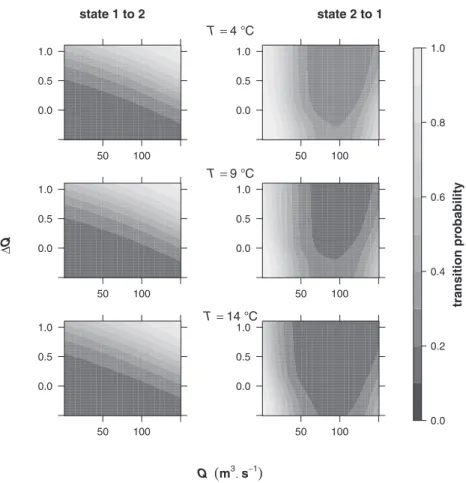
The spike-and-slab procedure confirms the importance of river discharge in migration triggering (Table 6). The main factor triggering the migration was relative change in river discharge (Fig. 5–left column): movements can be triggered even at low discharge when relative change is high. However, the transition probability from “active migrant” (state 2) to “pause state” (state 1) increased rapidly at low discharge (Fig. 5–right column). These results mean that eels start their migration during a rising river phase event and continue as long as the river flow remains at a sufficient level. Small movements are possible, even at low discharge if the relative change is high. For example, the probability for an eel to turn Table 5. Escapement rate (number of eels that escaped a reach/number of eels that entered the reach) for each reach and each eel downstream migration season. 2011–2012 2012–2013 2013–2014 Total REN-DRO 7/14 (50%) 7/14 (50%) DRO-PAU 5/7 (71%) 5/7 (71%) PAU-RIB 2/5 (40%) 16/19 (84%) 9/16 (56%) 27/40 (68%) RIB-EPE 1/2 (50%) 9/16 (56%) 9/9 (100%) 19/27 (70%) EPE-RAG 0/1 (0%) 8/9 (89%) 13/15 (87%) 21/25 (84%) RAG-NAD 6/14 (43%) 24/30 (80%) 21/24 (88%) 51/68 (75%) NAD-STA 2/6 (33%) 20/24 (83%) 19/21 (90%) 41/51 (80%) STA-CHA 2/2 (100%) 19/21 (90%) 19/19 (100%) 40/42 (95%) CHA-PAR 1/2 (50%) 19/20 (95%) 18/19 (95%) 38/41 (93%) PAR-ROC 1/1 (100%) 20/20 (100%) 18/18 (100%) 39/39 (100%) ROC-MON 0/1 (0%) 21/21 (100%) 16/19 (84%) 37/41 (90%)
Table 4. Last detected position of tagged eels depending on the release location (Fig. 1) and migration season.
Release REN Release PAU Release POL Total considered in the model Last detection 2011/2012 2012/2013 2013/2014 2011/2012 2012/2013 2013/2014 Before DRO 7* 0 Before PAU 2 2 Before RIB 3 3* 1* 3 Before EPE 1 4 0 5 Before RAG 1 1 2 3* 1* 0* 4 Before NAD 0 0 2 8* 5* 1* 2 Before STA 0 0 1 4 3 1 9 Before CHA 0 0 0 0 1 0 1 Before PAR 0 0 0 1 0 0 1 Before ROC 0 0 0 0 0 0 0 Before MON 0 0 1 1 0 2 4 Escapement 0 11 9 0 10 7 37 TOTAL 14 19 16 17 20 11 Total considered in the model 7 16 15 6 14 10 68
into active migrant is superior to 40% if the discharge increases from 5 m3/s to 10 m3/s (Fig. 5, left column, T = 4 °C first line),
which corresponds to half the yearly mean discharge, while this probability is equal to 56% if the discharge increases from 25 to 50 m3/s (Q90 of the spawning season !Table 1).
However, high levels of discharge are required for long-term movements: in our previous example the eel would pause a movement the following day with probability 92% if the discharge remains at 10 m3/s (Fig. 5, second column, T = 4°
first line), while this probability is equal to 33% if the discharge remains at 50 m3/s. This results in a rather limited
environmental window suitable for downstream migration.
Regarding transition from state 2 to state 1, the model predicts a decreased probability at very high discharge, however this corresponds to discharges greater than 100 m3/s,
i.e. greater than Q99 so very rare. Therefore, in this zone, the model is fitted on a very number of observations and predictions are very uncertain.
Temperature had a much more limited influence on our results, although it may have an influence on the transition from state 2 to state 1 (Table 6 –Fig. 5– right column). 3.3.3 Travelled distance and impact of obstacles
The model predicts that an active eel should theoretically travel tens of kilometres in 24 hours (Fig. 6) but this distance is significantly decreased by the presence of obstacles.
The posterior distribution of the penalty equivalent of an obstacle w is a way to quantify the impact of obstacles. The median value of 3.84 km would mean that each obstacle represents an additional 3.84 km. Given that there is an obstacle every 2 km, this would imply that the distance covered by active migrant in 24 h is divided by 2.86 because of obstacles. However, because the river is very fragmented and there is little contrast between reaches (Table 3), this impact was difficult to estimate as demonstrated by the flat posterior distribution of w (standard deviation: 2.4 km). It should also be noticed that this penalty is an average covering a wide range of impacts: some fish may suffer little impact while others may definitively stop their migration.
3.3.4 Activity indices
The model may be used to estimate (i) the proportion of actively migrant eels and (ii) the expected travelled distance (multiplication of the proportion of active migrant by the predicted travelled distance) to derive activity indices for each day of the three migration seasons (Fig. 7, we set peto zero, i.e.
no definitive stop since it would require knowing the date at which each eel starts to migrate and our estimate of pemight
include post-tagging effects). The low run-off in 2011–2012 resulted in a limited activity.Fig. 7 confirms that migratory activity is concentrated within limited windows of opportu-nity, especially in terms of expected distance travelled. Summing or averaging those indices illustrates the inter-annual contrast due to environmental conditions. For example, the average daily proportion of migrants was equal to 5.8% in 2011/2012, to 10.8% in 2012/2013 and 14.8% in 2013/2014. Regarding the total travelled distance (without accounting for definitive stop), it was equal to 47 km in the first season, 279 km in the second season and 433 km in the last season.
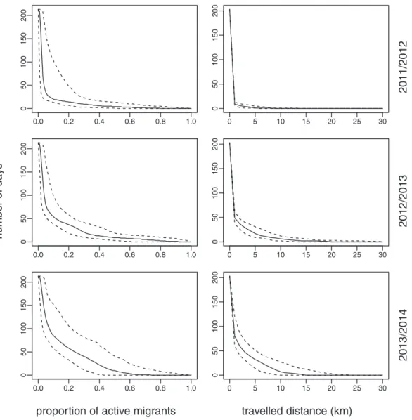
Another way to display the results consists in plotting the number of days in which the activity (proportion of migrants or travelled distance) was superior to a given level (Fig. 8). We observed that high activity is limited to a limited number of days, especially during the first season. The number of days in which half the eels were active was close to zero in 2011/2012 and around 20 days in the two following seasons. This was even worse regarding travelled distance: the number of days for which travelled distance was superior to 5 km was close to 0 in 2011/2012, close to 20 in 2012/2013 and about 40 in 2013/2014.
Table 6. Proportion of samples in which the environmental factors were selected as explanatory variables of states transition (state 1 = pause, state 2 = active migration).
State 1 to state 2 State 2 to state 1
Q 0.58 0.94 DQ 1.00 0.37 Tair 0.24 0.43 Q2 0.31 0.80 Tair2 0.28 0.46 2011/2012 eels 0 1 5 0 1 0 3 0 5 0 Q ( m 3 s ) 0 1 2 I ( km ) 2012/2013 eels 0 2 0 0 4 0 8 0 120 Q ( m 3 s ) 0 1 2 3 4 5 I ( k m ) 2013/2014 eels 0 8 20 60 100 Q ( m 3 s ) 0 2 4 6 8 1 0 I ( k m )
Nov Dec Jan Feb Mar Apr
0 20 60 100 0 2 4 6 8 10 Q(m3s) I ( km )
Fig. 4. Daily IðtÞ (light grey bars) for the three migration seasons (left panel) and corresponding river discharge (dashed lines). Dark grey bars represent the number of tagged eels used to calculate IðtÞ. Right panel represents the daily IðtÞ over the 3 seasons (when at least one tagged eel was available) as a function of river discharge.
3.3.5 Final states of non-escaped eels
It is interesting to analyse the estimated final states of the 31 eels that did not escape the studied area (Table 7). For 14 eels, a pause in the migration (state 1) was the most credible
state, or had credibility similar to a definitive abandon (state 3). For those 14 eels, mostly from the first migration season, unsuitable environmental conditions, especially low river flow, may account for the fact that they did not continue moving.
On the other hand, for 17 eels, the most credible states were either abandon (state 3) or still active migration (state 2), i.e. when migration had stopped completely (with no further movement, even in suitable conditions) or when eels were still actively migrating when last detected, but no further detections were registered. For those 17 eels, environmental conditions can hardly explain that they have not escaped the study site. Interestingly, 13 of those 17 eels were detected for the last time just a few kilometres downstream from one of hydropower plants, suggesting possible impacts caused by a passage through turbines (i.e. they may have been killed, injured or disoriented by turbines).
4 Discussion
Various environmental factors have been proposed as triggering factors of the downstream migration of silver eels (Bruijs and Durif, 2009): turbidity (Verbiest et al., 2012), wind direction (Cullen and McCarthy, 2003), pH (Durif et al., 2008), conductivity (Durif, 2003; Verbiest et al., 2012), rainfall (Durif, 2003; Trancart et al., 2013), temperature (Vøllestad et al., 1986; Reckordt et al., 2014), atmospheric pressure (Acou et al., 2008), moon phase (Poole et al., 1990;Cullen and
0.0 0.5 1.0 50 100 0.0 0.5 1.0 50 100 0.0 0.5 1.0 50 100 0.0 0.5 1.0 50 100 0.0 0.5 1.0 50 100 0.0 0.5 1.0 50 100 0.0 0.2 0.4 0.6 0.8 1.0 Q (m3. s−1) transition pr obability ∆ Q state 1 to 2 state 2 to 1 T = 4 °C T = 9 °C T = 14 °C
Fig. 5. States (state 1 = pause, state 2 = active migration) transition probabilities predicted by the model at different level of Q and DQ and different temperatures (4 °C, first line ! 9 °C which corresponds to the observed average, second line ! 14 °C, third line).
0 50 100 150 0 5 0 100 150 200 Q (m3 s-1) d is ta n c e ( k m ) .
Fig. 6. Theoretical distance that an active eel should travel in 24 h without any obstacle (median = solid black line, dotted black lines indicate the corresponding 95% credibility intervals) and distance travelled by an eel given the weirs density in the Dronne river (median = solid grey line, dotted grey line indicate the corresponding 95% credibility intervals) as estimated by the model as a function of daily discharge.
McCarthy, 2003; Acou et al., 2008), river flow (Cullen and McCarthy, 2003;Jansen et al., 2007; Acou et al., 2008;Bau et al., 2013;Reckordt et al., 2014). Most of those parameters are strongly linked: rainfall directly influences river discharge which in turn impacts turbidity and conductivity. As anywhere else, it is difficult in the River Dronne, to disentangle the respected effects of these correlated factors. Using controlled experiments, Durif et al. (2008) demonstrated that eels can display migratory behaviour while not exposed to river flow. They concluded that the main trigger is probably physico-chemical in nature. However, it is easier to predict rainfall than turbidity or conductivity. Consequently,Trancart et al. (2013)
used rainfall in their model to forecast migration activity and subsequently propose periods of turbine shutdowns. River flow can also be predicted using rainfall-runoff models (Beven, 2011) as illustrated by flood prediction models (Toth et al., 2000;Nayak et al., 2005). River flow is especially relevant, since it influences water speed and consequently affects migration speed. It also influences route selection when faced with an obstacle (Jansen et al., 2007;Bau et al., 2013;Piper et al., 2015), therefore also affecting the probabilities of
passing through alternative routes (weirs or by-pass devices for example). Consequently, this is a key factor in any model aimed at quantifying mortality caused by hydropower plants at both the obstacle and the river basin scales, as illustrated by the Sea-Hope model (Jouanin et al., 2012).
Interestingly, it was not river discharge itself, but the relative variation of river discharge which was selected by the model as the main triggering factor. This result is consistent withTrancart et al. (2013), whose study showed that rainfall triggers migration. It is indeed logical to assume that increased precipitation leads to a rising river flow phase. It may also be consistent withDurif (2003)andDurif et al. (2008): sediment concentration is often higher during a rising runoff phase than at an equivalent runoff during the falling phase. Williams (1989)refers to this as clockwise hysteresis. Such a hysteresis may explain why turbidity and conductivity, suggested as triggering factors byDurif (2003)andDurif et al. (2008), are different during rising and falling phases, and that the relative flow change selected in our model is just a distal mechanism that influences turbidity and conductivity which would be the proximal triggering factors. This significant direct or indirect
Nov Jan Mar May
0 5 0 100 150 Q
(
m 3 s)
2011/2012Nov Jan Mar May
0.0 0 .2 0.4 0.6 0.8 1.0 activ e migrants propor tion
Nov Jan Mar May
0 5 1 0 2 0 3 0 tr a velled distance (km)
Nov Jan Mar May
0 5 0 100 150 2012/2013
Nov Jan Mar May
0.0 0 .2 0.4 0.6 0.8 1.0
Nov Jan Mar May
0 5 1 0 2 0 3 0 Nov Jan Mar May 0 5 0 100 150 2013/2014 Nov Jan Mar May 0.0 0 .2 0.4 0.6 0.8 1.0 Nov Jan Mar May 0 5 1 0 2 0 3 0
Fig. 7. Average daily discharge (first line), daily proportions of active migrants (2nd line) and average expected travelled distance by eels (3rd line, the product of the proportion of active migrants multiplied by the predicted distance travelled by an active migrant gives an average distance travelled by eels) for each migration seasons (in columns). Thin dotted lines correspond to the 95% credibility intervals.
influence of river flow on migratory behaviour raises questions about the consequences of streamflow modification due to climate change (Arnell, 1999; Milly et al., 2005) and the impact of flow regulation due to different anthropogenic activities which smooth river flow variations, (this is especially true when dam reservoirs have high storage capacities and smooth variations at low discharges, though it is not the case in the Dronne River).
Our model quantifies the influence of different environ-mental factors, as well as making it possible to generate suitability envelop for migratory activity (Fig. 5–Fig. 8). The windows of opportunity for active migration are very limited (Fig. 7–2nd line !Fig. 8–left column) and even more limited when considering expected distance travelled (Fig. 7–3rd line !Fig. 8– right column). This has two main consequences. First, it confirms that, as proposed byTrancart et al. (2013), temporary and targeted turbines shutdowns can be a useful means of mitigating the impact of hydroelectric power stations in systems in which the hydrology and migration process are similar to the Dronne River. In practice, such a measure
requires two additional tools: a tool that predicts migration peaks 12–24 h in advance to comply with the operational delay for turbine shutdowns and a tool that estimates the distribution of eels within the river catchment to assess the number of eels likely to pass the obstacles. If such tools are available, turbine shutdowns have the advantage of not requiring any work on the obstacles. Therefore, this measure can be implemented quickly and has a limited cost if the number of migration peaks is limited. Turbine shutdowns should be considered as a possible solution among others such as fish-friendly trashracks (Raynal et al., 2013,2014) or other physical devices which are more multispecific and less site-dependent. Moreover, 75% of the time, eels entered or left our antenna fields between 20:00 and 07:00 am in our dataset. This type of nycthemeral behaviour was also observed byDurif and Elie (2008) andRiley et al. (2011). In view of this, shutting down turbines at night, when demand for power is lower, may or may not suffice depending on escapement targets. In all cases, simulation exercises are required to assess the ecological benefits of different management options, and costs-benefits (Dupuit, 1844;Snyder
0.0 0.2 0.4 0.6 0.8 1.0 0 5 0 100 150 200 0.0 0.2 0.4 0.6 0.8 1.0 0 5 0 100 150 200 0.0 0.2 0.4 0.6 0.8 1.0 0 5 0 1 0 0 1 5 0 2 0 0 0 5 10 15 20 25 30 0 5 0 100 150 200 0 5 10 15 20 25 30 0 5 0 100 150 200 0 5 10 15 20 25 30 0 5 0 1 0 0 1 5 0 2 0 0
proportion of active migrants travelled distance (km)
2011/2012 2012/2013 2013/2014 n u m b e r o f d a y s
Fig. 8. Number of days (y-axis) in which the proportion of active migrants is superior to a given level (x-axis) for each season (1st column) and number of days (y-axis) in which the expected travelled distance is superior to a given level (x-axis) for each season (2nd column). Dashed lines correspond to the 95% intervals and solid line to medians.
and Kaiser, 2009) or costs-effectiveness analysis (Crossman and Bryan, 2009) should be carried out to support decision making on each site or river.
Regarding migration triggering, a limit of our protocol is that our fish trapping devices caught already migrant eels and that may hinder our ability to work on migration triggering by environmental conditions. This was required for practical reason (existing trapping systems in the context of the “index river” system) but also for a question of battery life. However, eels are known to alternate between active migration and sometimes several weeks long waiting phases during their downstream migration depending on environmental conditions (Vøllestad et al., 1994; Durif, 2003; Watene et al., 2003;
Aarestrup et al., 2008; Verbiest et al., 2012;Reckordt et al., 2014). So even if catching active migrant eels, we were able to observe those switches between active migration and pause phases (the tables presented in Supplementary Material illustrates those switching) and then to derive the influence of environmental conditions on switching probabilities. Our study does not provide any information on the environmental
triggering of silvering process, but on the environmental triggering of silver eels movements. In our opinion, silver eel downstream migration should be considered as a three steps process: (i) silvering that occurs when eels have accumulated enough energy stores and after which eels wait for favourable conditions, (ii) activation/deactivation of migration due to favourable environmental conditions and (iii) travelled distance that depends on speed velocity and obstacles. It will be interesting in the future to catch and tag yellow eels and then track their downstream migration to explore the environmental triggering of silvering process and then of migration. However, this implied to have long-life tags, small enough to tag smaller fishes, with a large enough detection range and easily implantable to be able to tag a sufficient number of individuals. Unfortunately, it seems that such tags are not currently available.
In addition to environmental triggering of fish migration, the models also quantifies the impact of obstacles on travelled distance though the credibility intervals are very large, probably because of the lack of contrast between reaches. Table 7. Credibility of the three behavioural states estimated by the model for eels that have travelled more than 8 km but not escaped the studied area.
Possible causes Migration season eel id Wait Active Stop
Unsuitable conditions 2011/2012 1112_14 91% 2% 7% 2011/2012 1112_15 74% 2% 25% 2011/2012 1112_16 71% 1% 28% 2011/2012 1112_22 48% 1% 51% 2011/2012 1112_24 63% 2% 35% 2011/2012 1112_25 52% 47% 1% 2011/2012 1112_27 58% 3% 39% 2011/2012 1112_28 52% 1% 47% 2011/2012 1112_29 91% 2% 7% 2011/2012 1112_34 44% 1% 55% 2011/2012 1112_37 44% 1% 55% 2011/2012 1112_38 49% 1% 50% 2012/2013 1213_16 49% 2% 49% 2012/2013 1213_80 48% 1% 51% Unknown 2011/2012 1112_18 28% 1% 71% 2012/2013 1213_11 10% 1% 89% 2012/2013 1213_13 33% 5% 63% 2012/2013 1213_31 14% 85% 1% 2012/2013 1213_32 0% 0% 100% 2012/2013 1213_34 10% 0% 90% 2012/2013 1213_35 1% 0% 99% 2012/2013 1213_76 2% 0% 98% 2013/2014 1314_17 36% 63% 1% 2013/2014 1314_19 0% 0% 100% 2013/2014 1314_20 0% 0% 100% 2013/2014 1314_22 27% 72% 1% 2013/2014 1314_26 6% 0% 94% 2013/2014 1314_30 67% 3% 30% 2013/2014 1314_32 43% 3% 54% 2013/2014 1314_33 8% 0% 92% 2013/2014 1314_36 35% 64% 1%
In an obstacle free estuary,Bultel et al. (2014)observed mean directional migration of 48.6 km per day, a distance consistent with our estimates though the two systems are rather different. However, obstacles significantly impact the distance covered by eels and may lead to stops or delays in migration and, subsequently, potential mismatches between spawners arriving in the Sargasso Sea, notably between individuals located in the lower and upper parts of river catchments. It is more likely that the delay induced by obstacles impairs escapement success when there is a limited suitable window for migration, even though some silver eels are able to delay migration by up to a year to await favourable conditions (Vøllestad et al., 1994;
Feunteun et al., 2000). Consequently, quantifying the impact of obstacles should not be restricted to the quantification of turbine mortality as in the Sea-Hope approach (Jouanin et al., 2012) but also consider escapement failures due to delays induced by all kinds of obstacles (not only hydroelectric power stations, which represent about 5% of the obstacles listed in the French obstacles inventory). To achieve this quantification, a better knowledge on the time required to migrate to spawning grounds and on the continental escapement deadline would be necessary. The pattern of sex-ratio between the downstream (male biased) and upstream (more or exclusively females) area of a river catchment (Oliveira and McCleave, 2000; Tesch, 2003; Drouineau et al., 2014) combined with the impact of obstacles may also lead to arrival mismatch between males and females or to gender disparities in terms of escapement success. Increased energy costs and injuries caused by passing through downstream obstacles may also impair escapement success for silver eels, which stop feeding during reproduction migration (Bruijs and Durif, 2009).
In our study, a preliminary statistical analysis do not demonstrate any effect of fish length on escapement success, consequently, we did not include fish length in our model.
Palstra and van den Thillart (2010)demonstrated in a previous study that fish length is a main determinant of fish swimming capacity. Two reasons may explain this discrepancy. First, in our study, we only tagged silver eels large enough to tolerate the tag. It resulted in a restricted length distribution biased towards large individuals, limiting the contrast between individuals and impairing our ability to depict an influence of individual length. Secondly,Palstra and van den Thillart (2010)carried out in swim-tunnel and consequently on active swimming. In our field experiment, it is likely that silver eels have a passive or semi-passive swimming behaviour using river flow to carry out their migration and that consequently, fish length have a more limited impact on migration velocity and travelled distance.
We developed a Bayesian hierarchical model (or state-space model) to analyse the movements of tagged spawning eels. This kind of model has previously proved useful in analysing movements (Patterson et al., 2008), notably in the framework proposed by Nathan et al. (2008). The model enabled us to evaluate simultaneously the influence of environmental factors on migration triggering and the influence of river discharge on distance travelled in a unique integrated model (Fig. 3), while quantifying uncertainties. As mentioned in the introduction, the two aspects have generally been analysed independently depending on the type of available data. Analysis of migration from captures in a specific trap is suitable to analyse migration triggering (Acou
et al., 2005;Trancart et al., 2013) while radiotracking data are appropriate for analysing movements both in terms of distance travelled (Verbiest et al., 2012) and behaviour at specific dams (Jansen et al., 2007;Bau et al., 2013). The main strength of our study is that it analyses three elements simultaneously: migration triggering, distance travelled and the impact of obstacles. The model may be used in the future to predict proportion of active migrants and expected distance travelled by eels (Fig. 7, 3rd column !Fig. 8). Combined with a model of eels distribution within the catchment, they can be used to determine river discharge thresholds for turbine shutdown or to derive yearly indices of escapement success. The indicators proposed in section “activity indices” can be a first step towards such an escapement success index and show that in years of low discharges, the expected travelled distance is very limited, even without considering any source of mortality (Fig. 8). As mentioned earlier, simulation and cross-validations exercises would be necessary to validate the model prediction ability and to assess the relevance of such a mitigation measure.
One possible bias of most telemetry studies is the risk of misinterpretation due to mortality of tagged individuals and that could explain our limited escapement. Our protocol aimed at reducing post-surgery mortality (use of cyanoacrylate adhesive and antibiotic to limit the risk of post-surgery infection, limitation of time between catching and releasing fishes, limitation of fish transport and protocol that limit the risk of tag expulsion). Given the limited numbers of available eels for the experiment, it was not possible to carry out a true post-surgery experiment, however three eels were tagged with a similar protocol (but bigger tags) and kept in a tank with river water for 19, 25 and 44 days. They all survived and displayed normal healing of their incision. Though silver eel fishing is strictly forbidden in this river, mortality can also be induced by predation or hydropower plants during the migration. Contrary to traditional statistical approaches used to analyse telemetry data, the model allow to overcome this bias by introducing a third stage “definitive stop” that accounts for mortalities. Fishes that did not move at all despite favourable conditions were classified as “definitive stop” by the model and therefore were not “considered” when inferring the transition probabili-ties between active migration and pause states. Interestingly, the analysis of estimated final states by the model suggested a possible impact of hydropower plants.
The model predicts that small scale movements are possible at low level of discharge in a period of rising flow, but high levels of discharge are required to maintain migration activity and to increase travelled distance. As a consequence, estimated activity indices were nearly nil below 20 m3s!1. This value should not be
directly applied to rivers other than the Dronne. However, carrying out a meta-analysis of the different radio-telemetry experiments on silver eel migration would be a relevant way of identifying invariants between rivers, even though in large rivers and downstream systems, migratory behaviour patterns could be more difficult to interpret (and to link to environmental parameters) as they should be the consequence of different upstream behaviours linked to different hydrologies. Neverthe-less, state-space models are flexible enough to be applied in a wide range of situations and fitting such models to the other experiments would facilitate results comparisons and derive invariants. Using exceedance discharges rather than basic
discharges would appear to be a suitable way of carrying out such a meta-analysis.
Generally, state-space models have been used on movement data with high spatial and temporal resolution (Patterson et al., 2008;Jonsen et al., 2013;Joo et al., 2013), however they can still be used with sparser data (such as ours) to explore the interplay between individual internal state, environmental conditions, and resulting individual move-ments. More generally, it confirms that the movement ecology framework is an appropriate approach to explore this interplay in many fish radiotracking experiments in rivers.
Supplementary Material
Supplementary file supplied by authors. The Supplemen-tary Material is available at http://www.alr-journal.org/ 10.1051/alr/2017003/olm.
Acknowledgements. This study was funded by the Office National de l'Eau et des Milieux Aquatiques (Onema). The river index action plan for the River Dronne was funded by the “Agence de l'Eau Adour-Garonne”, the “Conseil Général de la Gironde” and by European Commission Feder funds. This plan includes the fish trapping program operated by the Onema, the “Syndicat Mixte d'Étude et d'Aménagement du Ribéracois”, the “Syndicat Intercommunal d'Aménagement Hydraulique (SIAH) Sud Charente : bassins Tude et Dronne”, the “Communauté de Communes d'Aubeterre” and Epidor. We are especially grateful to Pascal Verdeyroux (Epidor) for his involvement in fish trapping and for his remarks and comments about this paper. We would like to thank Patrick Lambert, Christian Rigaud, and Anne Drouineau for their participation in fruitful discussions and two anonymous referees for their comments and suggestions. We are also grateful to Eurocean and INRA networks on trajectories (Nicolas Bez ! IRD, UMR Marbec; Stéphanie Mahévas ! Ifremer; Marie-Pierre Etienne ! AgroParisTech, UMR MIA; Pascal Monestiez ! INRA) for their methodological support on trajectory analysis.
References
Aarestrup K, Thorstad E, Koed A, et al. 2008. Survival and behaviour of European silver eel in late freshwater and early marine phase during spring migration. Fish Manag Ecol 15: 435–440. Acou A, Boury P, Laffaille P, Crivelli A, Feunteun E. 2005. Towards a
standardized characterization of the potentially migrating silver European eel (Anguilla anguilla, L.). Arch Hydrobiol 164: 237–255.
Acou A, Laffaille P, Legault A, Feunteun E. 2008. Migration pattern of silver eel (Anguilla, L.) in an obstructed river system. Ecol Freshw Fish 17: 432–442.
Anonymous. 2010. Plan de gestion anguille de la France ! Application du règlement (CE) n°1100/2007 du 18 septembre 2007–Volet national. Ministère de l'écologie, de l'énergie, du développement durable et de la mer, en charge des technologies vertes et des négociations sur le climat. Onema: Ministère de l'alimentation, de l'agriculture et de la pêche.
Arnell NW. 1999. The effect of climate change on hydrological regimes in Europe: a continental perspective. Glob Environ Change 9: 5–23.
Baras E, Jeandrain D. 1998. Evaluation of surgery procedures for tagging eel Anguilla anguilla with biotelemetry transmitters. Hydrobiologia 371–372: 107–111.
Barton PS, Lentini PE, Alacs E, et al. 2015. Guidelines for using movement science to inform biodiversity policy. Environ Manag 56: 791–801.
Bau F, Gomes P, Baran P, et al. 2013. Anguille et ouvrages: migration de dévalaison. Suivi par radiopistage de la dévalaison de l'anguille argentée sur le Gave de Pau au niveau des ouvrages hydro-électriques d'Artix, Biron, Sapso, Castetarbe, Baigts et Puyoo (2007–2010). Rapport de synthèse.
Berge J, Capra H, Pella H, et al. 2012. Probability of detection and positioning error of a hydro acoustic telemetry system in a fast-flowing river: intrinsic and environmental determinants. Fish Res 125: 1–13.
Berger J, Young JK, Berger KM. 2008. Protecting migration corridors: challenges and optimism for Mongolian saiga. PLoS Biol 6: 1365–1367.
Beven KJ. 2011 Rainfall-Runoff Modelling: The Primer. Chichester, UK: John Wiley & Sons.
Bez N, Walker E, Gaertner D, Rivoirard J, Gaspar P. 2011. Fishing activity of tuna purse seiners estimated from vessel monitoring system (VMS) data. Can J Fish Aquat Sci 68: 1998–2010. Blackwell B, Gries G, Juanes F, Friedland K, Stolte L, McKeon J.
1998. Simulating migration mortality of Atlantic salmon smolts in the Merrimack River. North Am J Fish Manag 18: 31–45. Bolker BM, Gardner B, Maunder M, et al. 2013. Strategies for
fitting nonlinear ecological models in R, AD Model Builder, and BUGS. Methods Ecol Evol 4: 501–512.
Bonhommeau S, Le Pape O, Gascuel D, et al. 2009. Estimates of the mortality and the duration of the trans-Atlantic migration of European eel Anguilla anguilla leptocephali using a particle tracking model. J Fish Biol 74: 1891–1914.
Boubée J, Williams E. 2006. Downstream passage of silver eels at a small hydroelectric facility. Fish Manag Ecol 13: 165–176. Breukelaar AW, Ingendahl D, Vriese FT, De Laak G, Staas S, Klein
Breteler JGP. 2009. Route choices, migration speeds and daily migration activity of European silver eels Anguilla anguilla in the River Rhine, north-west Europe. J Fish Biol 74: 2139–2157. Briand C, Fatin D, Feunteun E, Fontenelle G. 2005. Estimating the
stock of glass eels in an estuary by mark-recapture experiments using vital dyes. Bull Fr Pêche Prot Milieux Aquat 378–379: 23–46.
Briand C, Fatin D, Fontenelle G, Feunteun E. 2003. Estuarine and fluvial recruitment of the European glass eel, Anguilla anguilla, in an exploited Atlantic estuary. Fish Manag Ecol 10: 377–384. Bridger CJ, Booth RK. 2003. The effects of biotelemetry transmitter presence and attachment procedures on fish physiology and behavior. Rev Fish Sci 11: 13–34.
Brown R, Cooke S, Anderson W, McKinley R. 1999. Evidence to challenge the “2% rule” for biotelemetry. North Am J Fish Manag 19: 867–871.
Brown RS, Eppard MB, Murchie KJ, Nielsen JL, Cooke SJ. 2011. An introduction to the practical and ethical perspectives on the need to advance and standardize the intracoelomic surgical implantation of electronic tags in fish. Rev Fish Biol Fish 21: 1–9.
Bruijs MCM, Durif CMF. 2009. Silver eel migration and behaviour. In: van den Thillart G, Dufour S, Rankin JC, eds. Spawning migration of the European eel, Fish & Fisheries Series. Netherlands: Springer, pp. 65–95.